Patient/Breast-Specific Detection of Breast Tumor Based on Patients’ Thermograms, 3D Breast Scans, and Reverse Thermal Modelling

Abstract

Background: Mammography is the preferred method for the diagnosis of breast cancer. However, this diagnostic technique fails to detect tumors of small sizes, and it does not work well for younger patients with high breast tissue density. Methods: This paper proposes a novel tool for the early detection of breast cancer, which is patient-specific, non-invasive, inexpensive, and has potential in terms of accuracy compared with existing techniques. The main principle of this method is based on the use of temperature contours from breast skin surfaces through thermography, and inverse thermal modeling based on Finite Element Analysis (FEA) and a Genetic Algorithm (GA)-based optimization tool to estimate the depths and sizes of tumors as well as patient/breast-specific tissue properties. Results: The study was conducted by using a 3D geometry of patients’ breasts and their temperature contours, which were clinically collected using a 3D scanner and a thermal imaging infrared (IR) camera. Conclusion: The results showed that the combination of 3D breast geometries, thermal images, and inverse thermal modeling is capable of estimating patient/breast-specific breast tissue and physiological properties such as gland and fat contents, tissue density, thermal conductivity, specific heat, and blood perfusion rate, based on a multilayer model consisting of gland and fat. Moreover, this tool was able to calculate the depth and size of the tumor, which was validated by the doctor’s diagnosis.

1. Introduction

One of the most common causes of disease-related death among young women in developing countries is breast cancer [1]. Changes in a cell genome can be caused by various factors such as hormonal dysfunctions or external causes, which lead to the development of cancerous cells. The most important factor is the stage of disease, as it plays an important role in treatment procedure and the recovery rate [2]. Genetic predisposition, a burdened family history, lack of childbirth experience, abortions, and age are the main risk factors that may cause the development of tumor, in addition to lifestyle with pernicious habits such as smoking, alcohol, obesity, lack of physical activities, etc. [3,4].

Figure 1 shows that breast cancer constitutes 11.7% among all cancer cases including both genders worldwide [5], whereas the mortality rate from breast cancer for females is 15.5% among all cases of cancer for females worldwide. It is proven that the early detection of breast cancer can be highly treatable. According to the stages of the cancer development process, patients with stages 2 and 3 of the disease were more common (84% in the compartment). This is due to the fact that stage 1 breast cancer is only determined during regular mammography checkup, without clinical manifestations.

Major methods of breast cancer diagnosis are mammography, ultrasound investigation, MRI, and biopsy. The main purpose of a biopsy is to determine if the tumor is benign or malignant. It involves a microscopic and histochemical examination of a tissue sample. This procedure is carried out after the discovery of the tumor.

Mammography is currently the most popular method. X-ray mammography is a classic version of mammography which has been used for several decades. X-ray mammography can be performed on a large number of women in a short time. This is ideal for mass preventive examinations. The procedure, which compresses the breast, is painful and uncomfortable. In addition, there are some limitations to its use. Firstly, this type of mammography is mainly recommended for older women above 40 years of age. This is because the images are more informative from this age due to the decrease in density of the glandular tissue of the mammary glands, which allow for the optimal transmission of X-ray radiation. This method is most effective for large tumors that are denser than surrounding tissues. Secondly, there is a potential threat of an adverse effect on a woman’s body, since this method uses ionizing radiation (X-rays). Therefore, it is recommended that X-ray mammography be performed no more than once a year.

Ultrasound examination uses high-frequency acoustic waves. The method is used as the main complementary method for the diagnosis of breast diseases to determine whether the lump discovered is a cyst filled with liquid or a solid tumor. Ultrasound is more effective for younger patients as their mammary glands have denser structure.

An MRI scan is best suited for young women who have a hereditary predisposition to breast cancer. Unlike mammography, magnetic resonance imaging is performed without X-ray radiation, and the effectiveness of MRI studies does not depend on the density of breast tissues. However, MRI is very expensive and can be found only in major hospitals of big cities.

The diagnosis of cancer in its early stages is crucial for its treatment. It is difficult to diagnose cancer in early stages due to the size of the tumor, which generally does not induce pain. Existing methods are not conducive for regular mass screening in short intervals, and they are not suited for regular breast self-examination (BSE) as promoted by WHO [6]. Some are harmful, painful, or uncomfortable, while others can be expensive and not readily available. The effectiveness of the approaches can also be dependent upon factors such as gland density. As a result, many breast cancer cases are discovered in the late stage when the tumor has become big enough to induce pain and other symptoms including lymph node damage, drawn nipples, and discolored or destructed breast skin [3]. Treatment in these stages can be challenging.

A non-invasive and inexpensive approach for early breast cancer detection is the examination of the breast skin surface temperature. Body temperature is a popular indicator that is used to check human health status. The effective usage of thermal data in clinical conditions can diagnose many illnesses [7,8,9]. It is well known that temperature distribution on the skin depends on factors such as blood perfusion, metabolic rate, and ambient temperature. Any abnormality such as tumor or inflammation can cause the atypical distribution of temperature on the skin surface. Tumors have higher heat generation rates compared with surrounding healthy tissues, thus allowing for the observation of non-homogeneity in breast thermograms with tumors [10,11,12,13,14,15,16,17,18,19,20,21,22].

The study by Prasad et al. [13] compared the accuracy of infrared thermal imaging (IRTI) and mammography. The results showed that mammography had higher accuracy (95.38%) than infrared thermal imaging (92.31%). At the same time, thermography was able to detect three cases of malignant tumor, whereas mammography could not.

Shrestha et al. [14] divided the breast into seven layers including the tumor tissue and studied the temperature distribution on the breast surface. It was concluded that in the case of applying dynamic thermography in order to improve tumor detection, the healthy tissue would reach the steady-state condition earlier compared with the tumor tissue.

Wahab et al. [15] created various models of breasts with different compositions of glandular and fibrous tissues. It was concluded that the composition of the mammary gland affects temperature distribution on the breast surface. Further work by Salamunes et al. [16] examined 123 females using Dual-Energy X-ray Absorptiometry and an Infrared camera. The results of the study revealed the influence of the fat percentage on the temperature distribution on the surface of the breast that is captured by IR camera.

Researchers [2,8,17,18,19,20,21,22] suggested that improvements in the quality of thermal cameras and the development of machine learning techniques can significantly enhance thermography as an adjunct tool for breast cancer detection. They also stated that thermography could achieve greater advancement if used in combination with segmentation, extraction, or numerical simulation.

According to Jiang et al. [17] and Bezerra et al. [18], numerical simulation allows for the study of the relationship between thermal behavior (heat generation, thermal conductivity, blood perfusion, etc.) and breast physiological states. The most important part of such study is geometrical modeling, as the model is used for the calculation and definition of the variables influencing the physiological change of the breast state. In this regard, it is important to use the real geometry of the breast, consisting of different layers [14,19,20,21].

Therefore, in this study, we propose that the combination of thermography and 3D scanning of the breasts can be used for the early detection of tumors and for further development of BSE through the miniaturization of the equipment and Artificial Intelligence (AI). By using temperature distributions on skin surfaces and the breast’s 3D geometry, it is possible to use reverse thermal modelling and finite element analysis (FEA) to identify the presence of tumors in human breasts. Finite element modelling (FEM) is mainly used for forward simulations in the performance of analyses. On the other hand, by combining FEM with optimization methods in reverse thermal modeling, it would be possible to determine personalized tissue properties, based on which reverse thermal modeling and design optimization can then be employed in order to determine the sizes and locations of breast tumors.

The novelty of this study lies in the development of a unique tool for the estimation of the depths and sizes of breast tumors using 3D scans of patients’ breasts and personalized tissue parameters such as density, fat/gland contents, specific heat, and conductivity through reverse thermal modeling. This tool consists of an FEM solver and optimizer, using thermograms and 3D breast scans as inputs. Optimization is used to search for optimal patient-specific parameters based on temperature distribution on the breast skin and for thermal modelling using FEM, which is called backward thermal simulation. For this study, the experimental procedure involved the collection of clinical data such as 3D models of the breasts and thermograms (skin surface temperature distributions). The temperature readings and 3D models of healthy breasts, personalized data such as thermal conductivity, specific heat, density, and blood perfusion heat loss rate were computed for each patient by using reverse thermal modeling, which combines FEM and design optimization. These parameters were then used for reverse thermal modeling through FEM and design optimization based on the patient-specific data obtained above to search for the sizes and depths of tumors. Each procedure included patient-specific data and diagnostic results from a medical doctor, which was then used to validate the method proposed herewith.

2. Clinical Data Collection

This study involves the collection of patient data (Figure 2a) in a clinic; surface temperature data was collected using a non-invasive infrared imaging camera and the scanned geometry of the breast was taken using a 3D scanner. The study was approved by Nazarbayev University Institutional Research Ethics Committee (identification number is 294/17062020).

The geometry of the breast was scanned by a smart 3D scanner called Sense 2 from 3D Systems (Figure 2b), which is a very light and easy-to-use scanner with excellent resolution, used for scanning objects from 200 to 2000 mm, and with a scanning accuracy of 0.9 mm. The front panel of the device is equipped with two cameras and an IR sensor. The scanner generates 3D models of the subjects being scanned by using image processing, while the IR sensors are used to measure the distance between the scanner and the patient. Temperature distributions on the breast skin surfaces were recorded by the thermal camera IRTIS-2000 ME (Figure 2c), which is used for medical research and in the diagnosis of a wide range of illnesses, including oncological diseases. Its temperature resolution for the entire field of view is 0.02 °C and its temperature measurement accuracy is 0.1 °C.

The collected information was used to generate 3D solid breast models to serve as input in the proposed diagnostic method for tumor diagnosis. The collection of data was conducted in the Oncology Center in Nur-Sultan city, Kazakhstan.

The 3D scanner exports data as surfaces in the STL format rather than full-sized 3D solid models. Therefore, the geometric data had to be manually processed in order to fully construct 3D solid breast models in a CAD system. A scanned model is shown in Figure 3 as an example.

The scanned surface model was then processed and manipulated in a CAD program, converting it into a full-fledged 3D solid model from which FEM meshes could be generated for FEA simulation and reverse thermal modeling (Figure 4).

3. Governing Equations

The human body continuously generates heat through metabolic processes. Heat exchanges among internal organs and the external environment occur through conduction, convection, and thermal radiation, which can be described by the energy conservation equation for bioheat transfer as follows:

$${\dot{Q}}_{generated}={\dot{Q}}_{stored}+{\dot{Q}}_{lost}+\dot{W}$$

(1)

where the term Q_generated stands for the rate of heat generated by metabolic process; Q_stored is the rate of heat stored in tissues and fluids; Q_lost is the rate of heat lost to the environment; and the work performed by the tissues is W, which can be neglected due to its low value.

During metabolic process, the heat generation rate ${\dot{q}}_m\left(\underset{\_}{x},t\right)$ varies in the range of 5–10,000 W/m³. Integrating heat generation rate over a control volume gives the following:

$${\dot{Q}}_{generated}={{\displaystyle \int }}_v{\dot{q}}_m\left(\underset{\_}{x},t\right)dv$$

(2)

where $\underset{\_}{x}$ stands for spatial coordinate and $t$ is time.

Heat stored in control volume is:

$${\dot{Q}}_{stored}={{\displaystyle \int }}_v\rho c\left(\underset{\_}{x}\right)\frac{\partial T\left(\underset{\_}{x},t\right)}{\partial t}dv$$

(3)

Fourier’s law of conduction as a form of heat loss over the control volume surface can be expressed as follows:

$${\dot{Q}}_{conducted}={{\displaystyle \int }}_{A}k\nabla T\left(\underset{\_}{x},t\right)·\widehat{n} dA$$

(4)

where $k$ is the thermal conductivity of the tissue.

Heat loss rate due to blood perfusion is also a component of heat lost to blood flow, according to Fick’s law:

$${\dot{q}}_{blood}={\rho }_b{c}_b{\dot{w}}_b\left(\mathrm{T}-T_v\right)$$

(5)

where ${\rho }_b{c}_b$ stands for blood heat capacity and ${\dot{w}}_b$ for volumetric blood perfusion rate; $T_v$ is the arterial temperature.

By substituting all the above equations into Equation (1) and converting the surface integration into volume integration with Gauss’ theorem, subsequently dropping the integrals when the control volume tends to zero, we will then obtain the Pennes bioheat equation [23] at a point in the space inside the breast in PDE form:

$$\rho c\frac{\partial T}{\partial t}=\nabla ·k\nabla T+{\rho }_b{c}_b{\dot{w}}_b\left(T-T_v\right)+{\dot{q}}_m$$

(6)

From the bioheat equation, it can be seen that in steady state conditions, the term on the LHS of Equation (6) disappears. The following equation describes the boundary condition on the skin surface for heat convection with the surrounding air:

$$-k\nabla T=h\left(\mathrm{T}-T_{ambient}\right)$$

(7)

where h is the convection coefficient, with an assigned value of 13.5 W/m² °C, according to [24].

4. Numerical Methods

The Pennes equation is reformulated as follows:

$$\rho C\frac{\partial T}{\partial t}+\nabla ·\left(-\overrightarrow{k}\nabla T\right)={\rho }_b{C}_b{w}_b\left(T_b-T\right)+{\dot{q}}_m$$

(8)

where

$\rho$	is tissue density (kg/m3);
$C$	is tissue heat capacity (J/(kg K));
$T$	is temperature (K);
$\overrightarrow{k}$	is tissue thermal conductivity tensor (W/(m K));
${\rho }_b$	is blood density (kg/m3);
$C_b$	is blood heat capacity ( J/(kg K));
$w_b$	is blood perfusion rate (m3/(m3s));
$T_b$	is temperature, arterial blood (K);
${\dot{q}}_m$	is metabolic heat source (W/m3).

To estimate the effects of density and specific heat of tissues, the transient heat transfer process should be considered [24].

A numerical solver for the bio-heat equation based on the Finite Element Method (FEM) was used. Considering Equations (6) and (7), a finite element model can be obtained as follows:

$${\iiint }_v\left(k_x\frac{\partial W_1}{\partial x}\frac{\partial T}{\partial x}+k_y\frac{\partial W_1}{\partial y}\frac{\partial T}{\partial y}+k_z\frac{\partial W_1}{\partial z}\frac{\partial T}{\partial z}-\left({\dot{q}}_m+{\rho }_b{C}_b{w}_b\left(T_b-T\right)\right)W_1+\rho c\frac{\partial T}{\partial t}{W}_1\right)dv+{∯}_S{h}_c\left(T-T_{ambient}\right)W_{1}ds=0$$

(9)

where V is the volume integral range, S is surface integral range, and W₁ is the weighting function used in the FEM spatial discretization scheme.

The following steps should be taken to determine the numerical solution: create the 3D geometry model of the breast; mesh the geometry; define tissue material, as well as thermal and physical properties; specify the boundary conditions of the model; and finally, solve the governing equation numerically.

5. Multilayer Model

Real breasts are not homogeneous in tissue types and material properties, and they consist of different layers of tissues, with different physical parameters. In this case, the use of a multilayer geometric model of the breast will increase the accuracy of thermal and reverse thermal modeling, improve the search for physical parameters, and enhance the study of the characteristics of the tumor. The proposed model consists of two layers: gland and fat (Figure 5). The aim of this study was to find the parameters of each layer and the volumetric percentage of the fat and gland in the breast.

6. Design Optimization Methods

A genetic algorithm is adopted in the optimization process in reverse thermal modeling to search for tissue properties, tumor sizes, and locations based on input breast surface temperature values measured by the IR camera. It is based on a biological evolutionary theory and numerically applied to optimization problems. The algorithm was originally developed by Johny Holland [25]. Its concept for the canonical genetic algorithm procedure is shown in Figure 6.

The first step is initialization, where the first population of search properties is generated randomly. From the population, x_i individuals are picked based on their probability to breed into the next generation. The probability is calculated by the relation of individual and total fitness values, which are estimated through thermal modelling based on the accuracies of their surface temperature predictions in comparison with the corresponding input measured values:

$$P\left\{x_i is selected\right\}=\frac{f\left(x_i\right)}{{{\displaystyle \sum }}_{j=1}^{m}f\left(x_j\right)}>0$$

(10)

The next step is to cross over selected individuals. Supposing there is a chromosome with length l. A random number c is picked from 1 to l. As an example, the first child’s chromosome is formed from the first c elements of the second parent, and the last l to c elements of the first parent. For the second child, the procedure is reversed. An example is shown in Figure 7.

The last step is to implement a mutation on each child’s chromosome. The random number v is generated between 1 and l, so that the v-th element in the gene randomly changes to 0 or 1, with probability ranging from 0.001 to 0.01. The procedure in Figure 6 is repeated until the fitness value is met [26].

7. Model Setup

In order to run numerical simulations, boundary conditions should be set according to experiment. During the collection of patient data, room temperature was recorded, therefore providing each simulation with its own ambient temperature (

Table 1. Experiment ambient temperature.

Patient Number	Ambient Temperature [°C]
1	26.60 ± 0.1
2	24.60 ± 0.1
3	20.77 ± 0.1
4	26.95 ± 0.1
5	26.21 ± 0.1

).

The convection coefficient was set at 13.5 W/m² °C, as stated earlier and according to a previous study [27]. The internal thoracic wall was set to a constant temperature for internal organs at 37 °C. The third component of the Pennes equation is internal heat release due to metabolism. Blood perfusion is defined as the volumetric blood flow, based on an average flow rate per volume of tissue, in an area that contains sufficient capillaries. Most tissues, including most of the skin and brain, have high perfusion, with a perfusion coefficient designated as w_b. These parameters are listed in

Table 2. Pennes equation parameters [27].

Parameter Name	Breast	Tumor
Blood perfusion (mL/s/mL)	0.0006	0.012
Arterial temperature (°C)	37	37
Metabolic heat generation (W/m3)	700	70,000

, according to [27]. In this study, two computational studies were conducted: the first part assumed that there was no blood perfusion, which means that w_b was zero; in the second part of the study, blood perfusion was added to the equation. Reverse thermal modeling with an optimization process and 3D breast geometry and thermograms as inputs will help to find patient-specific tissue properties, which are a key novelty of this study. The heat transfer parameters as thermal conductivity, specific heat and density, and blood perfusion coefficient and fat/gland contents were obtained from different patients by reverse thermal modeling with design optimization, as described above.

In the GA-based optimization, the number of samples for the first generation is 100, further generations consist of 50 samples, and the maximum number of generations is 20. The objective in the optimization was set to minimize the difference between computed temperature and temperature from experimental measurements from patients.

The FEM analysis was performed using Comsol Multiphysics with the following steps:

• Create new parametric material in Material library;
• Link with Solidworks to import 3D geometry;
• Set depth and radius of tumor parametric;
• Set simulation to transient;
• Generate mesh;
• Set constant temperature of 37 °C to thoracic wall;
• Set convection on breast skin surface;
• Set internal heat generation for tissues;
• Set temperature probes on skin surface.

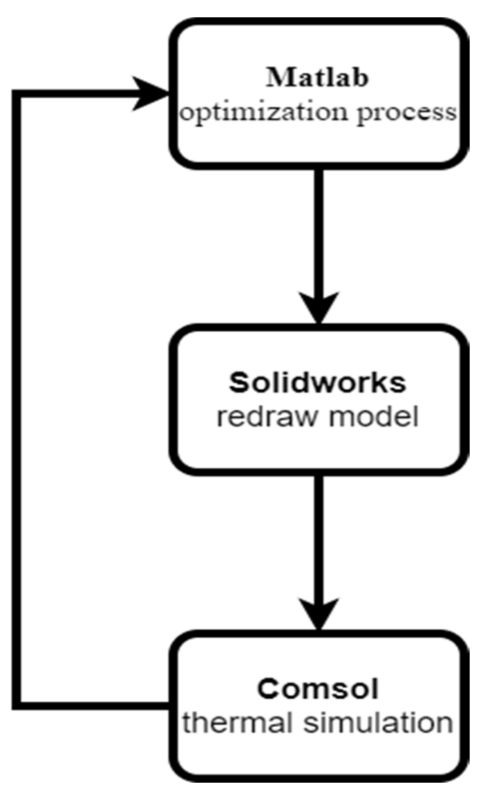
Comsol Multiphysics has an optimization tool based on stochastic and gradient-based methods. The disadvantage of those methods is that they can get stuck in local minimums. In order to overcome this problem, Comsol Multiphysics is coupled with MatLab Livelink, where MatLab can be employed for GA optimization while Comsol Multiphysics is used for finite element analysis. MatLab is capable of performing the optimization process, while MatLab Livelink can make the MatLab optimizer and the Comsol FEM solver communicate to perform the optimization and FEA simultaneously in order to achieve the objectives of finding patient-specific tissue properties and tumor sizes and locations. Additionally, this tool also requires Solidworks Livelink, so that the tumor model can be moved inside of 3D multilayer model in the optimization design parameter search, which is then redrawn by the CAD program and imported into the FEA program again for subsequent FEM mesh regeneration and FEA computations in the whole optimization loop (Figure 8). The fitness function for MatLab is presented in Algorithm 1.

Algorithm 1 The fitness function for MatLab

function y = function name(x) import com.comsol.model.* import com.comsol.model.util.* model = mphload(‘filename’) model.param.set(‘Parameter_1′, x(1)); model.param.set(‘Parameter_2′, x(2)); model.study(‘std1’).run; T = mphinterp(model,’T’, ‘coord’, [x,y,z]’); Temp = T(end); y = abs(Temp − Temp_exp); end

The first line defines the name of the function y. Code lines from the second to the sixth open the Comsol model and set the required parameters. The line “model.study(‘std1’).run” activates the simulation, and the code mphinterp(model,’T’, ‘coord’, [x,y,z]’) extracts temperature values from given coordinates. Finally, the fitness function y is the absolute value of differences between the computed and experimental temperatures.

Thus, the research methodology is demonstrated in Figure 9, which summarizes all the stages of the integrated diagnostic tool.

8. Results and Discussion

In this study, five patients’ data were used to perform the patient-specific reverse thermal modeling and tumor diagnosis in order to demonstrate the capabilities of the technique developed and to validate the models built.

Table 3. Age and demographic details of each patient.

Patient Number	Age	Sex	Number of Pregnancy	Number of Births	Age of First Birth	Family History of Breast Cancer	Age of Onset of Menstruation	Age at Menopause
1	59	Female	5	2	25	1	14	53
2	45	Female	9	7	19	0	12	Not started
3	59	Female	5	2	25	1	14	53
4	58	Female	4	3	22	0	12	49
5	52	Female	3	2	23	0	12	51

demonstrates the age and demographic details of each patient.

A mesh convergence study should be conducted before the analysis is performed so that the simulation results will not be improperly influenced by the mesh generated; simultaneously, computational efficiency and numerical accuracy can be achieved. In order to find the optimal number of elements for running a simulation, the temperature probes were performed at the nipples to check the predicted temperature values for convergence. By increasing the number of elements, differences between readings at the probes were compared, until an average difference of 1% was reached.

Table 4. Mesh convergence study for patient number one.

Number of Elements	Temperature	Difference (%)
280,414	34.01
320,584	35.3	3.79
401,383	34.55	2.12
442,842	34.2	1.01

shows the mesh convergence process for patient number one.

Table 5. Number of mesh elements for each breast.

Breast Number	Number of Elements
1	442,842
2	524,347
3	482,453
4	543,214
5	498,210

presents the results of the mesh convergence study, which shows the optimal number of elements for patients’ breast models with which mesh convergence was achieved.

Table 6. Estimated parameters of the homogeneous model.

Patient	Conductivity [W/m °C]	Density [kg/m3]	Specific Heat [J/kg °C]	Blood Perfusion [mL/s/mL]
1	1.49	901.51	2201.51	0.00015794
2	1.34	951.26	2010.48	0.00011972
3	1.14	997.24	1812.25	0.00010012
4	1.25	998.67	1849.25	0.00010876
5	1.32	1047.82	1797.17	0.00010172

includes the extracted tissue parameters of three patients’ breasts using reverse thermal modeling; these were based on a homogeneous model using the healthy breast’s data as inputs. The parameters were subsequently used as initial guesses for a multilayer model simulation to estimate the specific tissue parameters of each layer in the diseased breast.

Using the homogeneous breast model’s parameters as initial guesses, specific parameters of gland and fat, including conductivity, density, specific heat, and blood perfusion rate, were estimated (

Table 7. Estimated specific breast parameters (patient #1).

	Conductivity [W/m °C]	Density [kg/m3]	Specific Heat [J/kg °C]	Blood Perfusion [mL/s/mL]	Fat %
Gland	1.57	898.68	2357.69	0.00016652
Fat	1.32	919.62	2106.58	0.00014267	64.6

,

Table 8. Estimated specific breast parameters (patient #2).

	Conductivity [W/m °C]	Density [kg/m3]	Specific Heat [J/kg °C]	Blood Perfusion [mL/s/mL]	Fat %
Gland	1.50	978.62	2059.69	0.00012619
Fat	1.20	925.62	1982.65	0.00011652	52.7

,

Table 9. Estimated specific breast parameters (patient #3).

	Conductivity [W/m °C]	Density [kg/m3]	Specific heat [J/kg °C]	Blood perfusion [mL/s/mL]	Fat %
Gland	1.26	1005.65	1924.65	0.00011619
Fat	1.07	952.61	1661.62	0.00009616	67.62

,

Table 10. Estimated specific breast parameters (patient #4).

	Conductivity [W/m °C]	Density [kg/m3]	Specific Heat [J/kg °C]	Blood Perfusion [mL/s/mL]	Fat %
Gland	1.31	1010.14	1997.4	0.00011731
Fat	1.20	987.21	1701.1	0.00010021	61.1

and

Table 11. Estimated specific breast parameters (patient #5).

	Conductivity [W/m °C]	Density [kg/m3]	Specific Heat [J/kg °C]	Blood Perfusion [mL/s/mL]	Fat %
Gland	1.41	1101.25	1891.21	0.00010514
Fat	1.23	994.4	1703.14	0.00009831	51.4

). Based on the estimated fat layer dimension, the content of gland and fat were calculated in percentage.

The results of the above-mentioned GA-based reverse thermal modeling for the estimation of the sizes and locations of tumors, and the accuracy of the method are provided in

Table 12. Estimated tumor depth and diameter compared with the doctor’s conclusion.

Patient No.	Computed Tumor Size [mm]	Doctor’s Size [mm]	Computed Depth [mm]	Percentage Error (Tumor Size) [%]
1	23	up to 25	23.78	8
2	42	45	31.99	6.7
3	21.5	23	28.18	6.5
4	17.5	16	23	9.3
5	16.1	15	25.1	7.3

. Since the doctor’s examination was performed only by palpation and the given sizes are estimations made during this procedure, the presented reverse modeling results are considered to be in good agreement with the doctor’s diagnosis. In the case of patient one, the computed diameter of the tumor is 23 mm, while the doctor’s estimation was up to 25 mm. For patient two, the calculated diameter is 42 mm, which can be validated by the doctor’s approximation of around 45 mm. In case of patient three, the computed tumor diameter is 21.5 mm, which is close to the doctor’s palpation result of 23 mm. On average, the percentage error of the tumor method is about 0.23%.

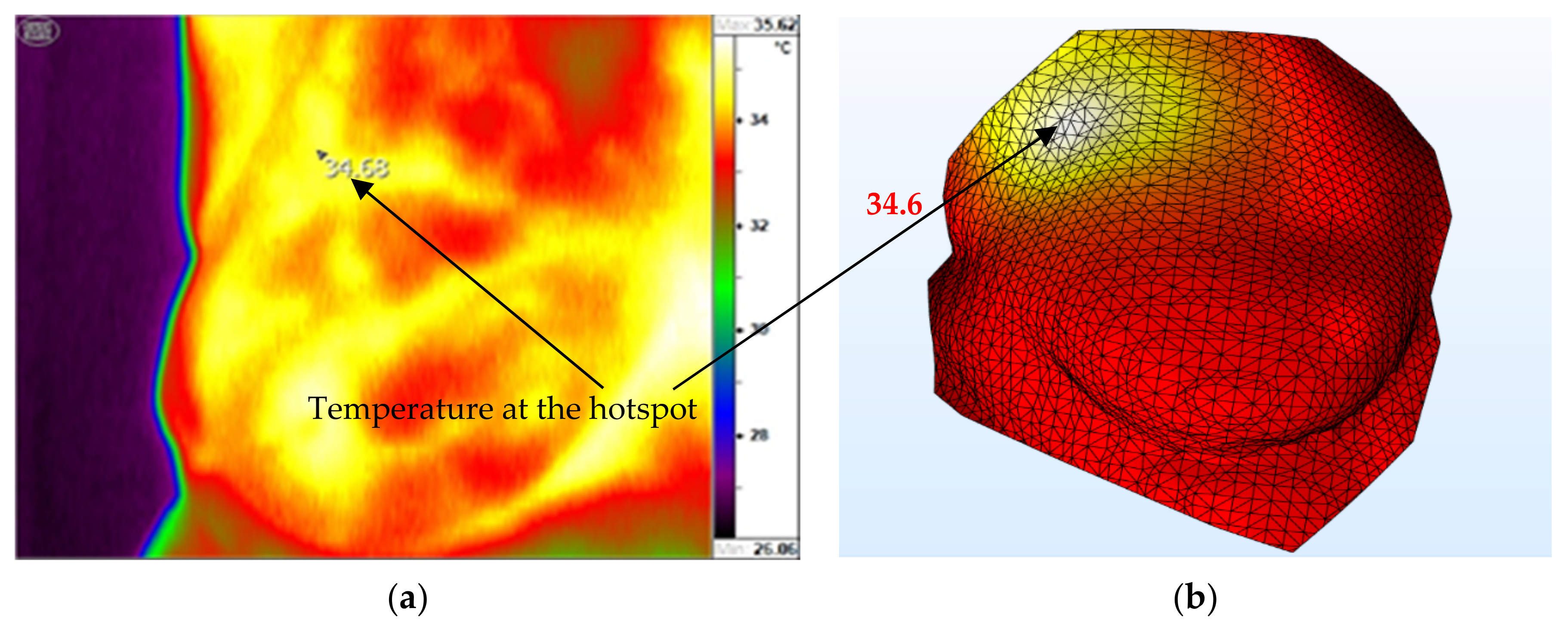
Figure 8 shows a comparison of the measured (Figure 10a) and computed (Figure 10b) temperature distributions for patient one with tumor in the breast. In general, the distributions of temperature and the locations of the hotspots between the two are in close agreement. However, we can see some small differences in the shapes of the hotspots; this can be caused by the non-uniform blood perfusion and distribution of vessels in the real breast, while thermal models are uniform in blood perfusion. The computed temperature at the hotspot is 34.6 °C, which is validated by the thermographic hotspot temperature with almost the same temperature, resulting in a percentage error of only 0.23%.

In general, the measured (Figure 11a) and computed (Figure 11b) temperature distributions for the second patient’s breast match, while the temperature at hotspot was calculated as 34.8 °C. However, the predicted temperature distribution is also quite uniform compared with the thermogram, which may be due to the non-uniform blood perfusion and vessel distribution in the real breast in comparison with the uniform perfusion in the model, as previously discussed. The numerical model was validated since the location and temperature of the hotspot agree well with the corresponding measurements; the percentage error was at 0.43%.

Figure 12 shows a comparison between the measured breast temperature distribution (Figure 12a) and estimated multilayer model prediction (Figure 12b) for the third patient. The doctor concluded that the tumor is located in the upper left quadrant, which can also be seen as a hotspot in the multilayer model prediction. As in the two previous cases, the highly irregular small temperature distribution in the real breast cannot be captured by the model due to the uniform blood perfusion assumption used.

In Figure 13, a comparison of the thermal image (Figure 13a) and computed (Figure 13b) temperature contours for patient four is presented. In the thermogram, the temperature at the hotspot is 34.42 °C, while the computed temperature at that point is 34.5 °C, which is very close to the former with a percentage error of 0.23%. In addition, the locations of the hotspots in both the thermogram and the predicted contours agree well.

The comparison of temperatures for patient five, can be seen in Figure 14. The hotspot temperature of the thermogram is 33.06 °C (Figure 14a), while the computed hotspot temperature is 33.16 °C (Figure 14b); percentage error is thus at 0.30%. Furthermore, the measured and predicted hotspot locations also agree with each other in the upper-left quadrant.

Figure 15, Figure 16, Figure 17, Figure 18 and Figure 19 show the 3D models of the five patients’ breasts with the computed parameters of the gland and fat layers, and the tumors. In the case of patient numbers one and two, the tumors are located at interfaces between the fat and gland layers. Patient number three has the tumor in the fat layer, while in Figure 18 and Figure 19 the tumors are located in the gland.

The proposed tool for tumor detection shows its usefulness based on the real patient data. The presented results are based on two kinds of breast models: homogeneous and multi-layer models. The homogeneous model was used as a starting point in the calculation of parameters such as conductivity, density, specific heat, and blood perfusion rate. The calculated parameters enabled the estimation of the tumor size and its location. Subsequently, the content percentage in the multi-layer model was determined. The final results were then validated by the doctor through medical examination and thermograms. The developed tool for the estimation of tumor depth and size, which makes use of real patient models and personalized physical parameters such as density, specific heat, and conductivity could be employed in further clinical trials with large sample sizes. For future studies, there is an ongoing effort to collect and generate more patient-specific data for machine-learning-based methods as well as for the validation of the current methods.

9. Conclusions

Reverse thermal simulations performed with the Genetic Algorithm-based optimization tool were used to estimate the personalized parameters of patients’ breasts, such as thermal conductivity, density, specific heat, and blood perfusion coefficients in gland and fat layers, which included the breast’s fat/gland contents along with 3D breast geometry and thermograms as inputs. The study was initially conducted with a homogeneous model using real patients’ data to estimate initial guesses of tissue properties for further simulation with a multilayer model. Simulations were later performed using Comsol Multiphysics with MatLab Livelink and Solidworks Livelink in an integrated optimization loop. Firstly, based on temperature contours from the healthy breast, the personalized breast parameters were estimated and then used as initial guesses for further simulation with a multilayer model of the healthy and diseased breasts. Using those parameters, patient-specific/breast-specific parameters and contents of each layer were predicted by the reverse thermal simulation. Finally, based on the estimated specific parameters of each breast, further reverse thermal modeling simulation was performed using Genetic Algorithm and the temperature distribution on the skin as input in order to predict the depth and size of the tumor. The predicted parameters agreed well with doctor’s diagnosis through palpation. A comparison of computed and IR thermographic temperature distributions shows general consistency as well as the very good agreement of predicted and measured temperatures at hotspots. Thus, it is concluded that the breast tumor diagnostic tool developed, which is based on patient-specific reverse thermal modeling, can accurately generate patient/breast-specific tissue properties and predict the size and location of the tumor in the breast.

Future study will include the collection of a large volume of patients’ data and the subsequent construction of thermal breast models for further validation and clinical trials. A Physics-Informed Neural Network (PINN) simulation tool will also be developed for comparison with the method developed for this study, and to allow for better prediction of the complex blood perfusion. More sophisticated breast models that contain different layers with an irregular distribution of vessels may be considered. Future study will also include the miniaturization of the equipment and the implementation of AI for BSE, as promoted by WHO. Our long term goal is to diagnose tumors with single-digit diameters and arbitrary depths during BSE.