1. Introduction
This paper compares a vortex ring theory (VRT) that is not based on the general momentum theory to the existing actuator disk theory (ADT) [
1] and the rotating annular stream-tube theory (RAST) [
2,
3]. The ADT and the RAST, whose origins are discussed hereafter, rely on the axial momentum balance in their formulation. The VRT is different from the ADT and the RAST in the sense that these two theories rely on the idealization that the wind speed at the wind turbine’s (WT) rotor is the average of the wind speed in the wake and the free-stream speed of the wind upstream of the WT. The VRT considers the fact that the wind slows down as it flows past the WT, resulting in an induction or interference factor due to solidity
as, and that a further reduction in the wind speed occurs in the wake, resulting in an axial induction factor due to wake rotation
aw. There is also a tangential or azimuthal component of the induction factor due to wake rotation
a’, commonly called the azimuthal or angular induction factor. The RAST also makes use of the angular induction factor. Thus, per the VRT, the axial induction factor at the WT wake is
δ = as + aw and not twice the induction factor at the WT rotor. It is worth noting that for
a = 0.5, the freestream speed in the axial direction at the Trefftz plane is zero in the cases of the ADT and the RAST, whereas it is non-zero in the case of the VRT because
as = 0.5 does not necessarily result in a
δ = 1. The VRT represents the wake of a horizontal-axis WT (HAWT) with a conical control volume (CV) and applies the Biot–Savart law [
4] to the CV to determine
a’ and
aw. The CV is a conical helix since the flow past a WT rotor is solenoidal and a potential flow. This conical CV should not be misconstrued to be a diffuser, as is typical of shrouded WTs. The intent of this paper is to delve into the aerodynamics of commercial-scale unshrouded WTs. The axial momentum balance across the rotor of a HAWT forms the basis upon which Rankine formulated the ADT [
1]. He represented the rotor with a permeable disk of cross-sectional area
A, which extracts energy from the air flowing past it by reducing its pressure. Upstream the HAWT, the air pressure is above atmospheric due to the slowing down of the airstream. As the airstream passes through the WT, it loses pressure [
1]. Improvements on this theory were made by Froude [
5] who included the effects of the wake in his calculations and stated that the induced velocity at the wake of an actuator disk is twice the induced velocity at the disk.
Chattot [
4] attempted to extend the ADT to unsteady fluid flow. In his treatise, he expatiated on both the steady and unsteady flow past a HAWT using a vortex tube as his CV. The vortex tube consisted of a continuous succession of vortex rings shed by the rotor and carried downstream by the flow. Suffice it to say, Chattot’s CV is quasi-cylindrical and does not seem to account for the expansion of the flow resulting from the slowing down of the air as it passes through the rotor. After rigorous mathematical manipulations, this researcher showed that at steady state, the induced velocity downstream the rotor at the Trefftz plane is twice the induced velocity at the rotor.
In his bid to estimate the maximum power extracted by a HAWT, Betz used the one-dimensional mass conservation and momentum conservation laws in conjunction with the ADT first developed by Rankine and Froude for propellers [
5]. Other schools of thought [
1] hold that the ADT is the brainchild of Rankine. The Betz model dwells on the premise that the power extracted by the WT is solely derived from the pressure drop across the rotor. This pressure drop results in a static thrust on the rotor [
6]. Alternatively stated, a fluid particle passing through the WT rotor loses part of its kinetic energy (KE), viz, the flow through a WT slows down gradually from an upstream free-stream speed of
U0 to an average value far downstream in the wake
Uw. The static pressure increases from its upstream value
P∞ to a value
Pr+ just in front of the rotor and then drops to
Pr− behind the rotor. The difference in static pressure between the rotor inlet and its outlet results in an axial force exerted on the rotor. Recovery of the pressure lost by the wind as it flows past the WT occurs gradually in the wake until the initial free-stream pressure
P∞ is attained. It is worth noting that
Pr+ − P∞ > P∞ − Pr− [
7].
The flow past a WT rotor is decelerated. Ideally, this deceleration of flow can result in a maximum power extraction of 59.26% of the initial KE per unit time of the wind by a WT rotor as established from the ADT, which is based on the conservation laws of flow as discussed in the foregoing paragraph. As stated earlier, the ADT replaces the WT rotor with a permeable disk with a distributed load, yielding the same overall thrust as the actual rotor. Despite this far-reaching abstraction, the ADT is the basis of WT aerodynamics. The maximum efficiency achievable by a HAWT is attributed to Betz by most German and British scholars, while Russians attribute it to Joukowsky [
8]. In their bid to achieve good analytical results, Keane et al. [
9] developed an analytical method predicated on the conservation of mass and linear momentum in the context of the ADT and the assumption that the velocity deficit in the wake follows a double Gaussian distribution.
Existing versions of the VRT, typically called ring vortex theories, predicate on the fact that the axial induction coefficient at the wake is 2
a or in other words the wind speed at the wake of a WT is
Uw = U0(1
− 2
a). A case in point is the ring vortex actuator disk model by Bontempo et al. [
10]. Bontempo et al. [
10] proposed a ring-vortex actuator disk theory (RVADT) based on a uniformly loaded disk with no wake rotation, predicated on the axial and generalized momentum theories, respectively. They used their theory to numerically investigate the effects of the hub of HAWTs on the flow past a WT rotor. Per these researchers, the hub blockage effects are more pronounced in small HAWTs whose hub radius to rotor radius ratios range between 25 and 30% than in large HAWTs, which typically have hub radius to rotor radius ratios ranging between 4 and 5%. These researchers assert that hub blockage effects on large HAWTs are lower than those of smaller HAWTs such that neglecting these effects has little impact on the solution for large HAWTs than for smaller HAWTs. The RVADT models the flow induced by the rotor disk and hub with ring sheet vortices, which are discretized through a classical panel method by utilizing a homogeneous Dirichlet boundary condition for the velocity just beneath the hub vortex sheet, while a free force condition is imposed along the entire boundary [
10].
These actuator disk-based ring vortex theories have a drawback in the sense that when a = 0.5, the axial component of the wind speed at the wake is zero, something that causes the air particles to stagnate at the Trefftz plane and undergo circular motion. This is not what occurs in real life. The proposed VRT does not result in a zero axial wind speed at the wake when the interference factor is 0.5 because the induction factor due to wake rotation aw is not necessarily 0.5.
Other models have been used by numerical analysts to study WT wakes. Wake modeling approaches include empirical correlations, the ADT and full three-dimensional computational fluid dynamics (CFD) simulations. Analytical methods, such as Glauert’s blade element momentum theory (BEMT), have been extended to computational WT models, such as the vorticity–velocity model (VVM) [
9]. The BEMT combines a CV conservation of momentum analysis with the blade sectional analysis [
11]. The BEMT is an upshot of the general momentum theory developed by Glauert and Joukowsky [
5,
12]. Although interesting solutions of the general momentum equations were developed for special cases with simplifying assumptions, these researchers were not able to provide closure with an analytically determined axial force equation; later researchers determined that there was not enough information to account for an axial force balance [
12]. According to the BEMT, the axial induction factor varies radially and azimuthally across the rotor [
9]. Another numerical model is the actuator line model (ALM). The ALM represents the three rotor blades of a HAWT by a rotating body of forces. The force per unit span on a rotor blade is estimated and the total force on the rotor is calculated by multiplying the integral of the force per unit span by the number of rotor blades [
13]. Typically, the overall forces on a WT rotor are calculated by adding up the aerodynamic forces of each cross-section using the strip or blade element theory. The centrifugal and Coriolis forces that appear in the laminar boundary layer (LBL) increase the aerodynamic lift forces as compared to those in a similar two-dimensional non-rotating disk. Centrifugal forces produce a span-wise outward velocity, which gives rise to the Coriolis forces that act as favorable pressure gradients in the chord-wise direction. They also tend to reduce the thickness of the LBL due to the outward movement of the fluid, viz, the centrifugal pumping effect. This secondary flow postpones the appearance of the separation point, allowing the airfoil to reach a higher angle of attack before stalling [
14]. Glauert assumed that the angular speed of the wake is never greater than the angular speed of the rotor [
12] but gave no justification for this assumption. On the contrary, in real life, even static rotors impart swirl on their wakes [
12].
A setback of the ADT is the fact that it results in a discontinuity in pressure as air flows past the actuator disk. The Betz–Joukowsky limit was derived using a simple balance of axial momentum and remains the basis for the maximum power extracted by an ideal HAWT rotor [
15]. Chamarro et al. [
16] modified the ADT in their bid to account for the effects of the atmospheric boundary layer (ABL) on the maximum efficiency of an ideal HAWT by introducing modification factor
β to account for the effects of Coriolis forces on the average KE per unit mass passing through the rotor and modification factor
γ to account for the effects of velocity changes over a cross-section of the CV on the average momentum. They claimed that because of the effects of the ABL, the maximum power coefficient calculated is slightly higher than the Betz–Joukowsky limit—i.e., a 1–2% increase in the Betz limit was observed.
Simisiroglou et al. [
17] in their study of the analytical methods for WT wake developed independently by Jensen and Larsen, discovered that though these models are fast in calculating wake velocity deficit, they rely solely on empirical coefficients that are case specific. For instance, Jensen’s model requires a wake expansion coefficient to be determined. These two models are modifications of the ADT. Larsen considered a turbulent wake state in developing his model, while Jensen used a steady wake state. Power predictions by the latter are higher than those of the former.
By revisiting the ALM discussed in a foregoing paragraph, it was first developed by Sorensen and Shen in 2002. It represents the HAWT rotor blades by a series of point forces acting along the span of each rotor blade at the quarter chord. The ALM allows for the flow effects on the rotor blades to be modeled using discrete rotor blades without requiring the discretization of the blade boundary layer, resulting in lower computational requirements than three-dimensional blade-resolved models, while preserving the principal effects of the rotor on the flow. The ALM is implemented by discretizing each rotor blade into span-wise segments. The blade element method (BEM) is used in conjunction with the flow field data returned by a Reynolds Average Navier–Stokes (RANS) solver to estimate the two-dimensional aerodynamic forces acting at the quarter chord of each span-wise segment. The force on each segment of radius
r and length
δr is the vector sum of the lift and drag. The ADT, the BEMT and three-dimensional blade-resolved methods are frequently used in the simulation of the flow past HAWT rotors. The ADT and the BEM allow for fast simulations but do not accurately simulate flow features, such as unsteady wake development [
18]. The BEMT neither accurately predicts the axial velocity of flow past a HAWT rotor, especially around the inner part of the rotor where wake rotation accelerates the flow and the outer part where it decelerates the flow [
19].
It is worth noting that the ABL is quite stable under nocturnal conditions, so much so that a considerable shear develops with an increase in wind speed as the height above the ground increases. Shear in the wind entering large HAWTs with mega-watt capacities is a frequent operational condition. Simulating such inflow conditions using the BEM, as is typically done using most common aero-elastic codes, is fraught with uncertainty. This uncertainty is the upshot of the lack of a well-documented procedure of the BEM model for sheared inflow [
20]. Yet another method for simulating the flow past HAWTs is the actuator sector method (ASM). The ASM distributes the forces applied to the fluid azimuthally to maintain a continuous flow solution for increased time steps compared to the ALM. It is a hybrid actuator model that preserves the features of the ALM and reduces the computational expense associated with small time steps, which are typical of the latter. The ASM is the intermediary between the ALM and the ADT [
21].
In this paper, a comparison is made between the ADT and the RAST derived by others [
2,
3] and the VRT. To carry out the comparison, the design parameters of the United States Department of Energy’s National Renewable Energy laboratory’s (NREL) 5 MW reference offshore WT (OWT) are used. The WT to be investigated in this work is an upwind, three-bladed, 5 MW NREL reference HAWT. The OWT has a swept radius of 63 m, a hub height of 90 m, a hub diameter of 3 m, a cut-in rotational speed of 6.9 RPM and a rated rotational speed of 12.1 RPM. Its cut-in wind speed at 90 m hub height is 3 m/s, its rated wind speed at hub height is 11.4 m/s and its cut off wind speed is 25 m/s [
22].
This paper is structured as follows:
Section 2 is a critique of the generalized momentum theory that forms the basis for the ADT and the RAST.
Section 3 and its subsections consist of the derivation of the basic equations of fluid dynamics from which the aerodynamic equations are developed.
Section 4 outlines the steps followed in coding the necessary equations into MATLAB and the subsequent plotting of curves.
Section 4 consists of the parameters of the 5 MW reference NREL OWT.
Section 5 consists of the results and discussion of the results of the analysis based on the three theories; subsection below
Section 5 is a comparison between the VRT results and existing numerical and experimental results.
Section 6 is the conclusion of the paper.
2. Critique of Generalized Momentum-Based Theories
The generalized momentum-based theories rely on assumptions that only make mathematical sense and defy the law of conservation of momentum. Elementary mechanics reveals that if a given mass of air m, moving with a speed in the axial direction, impinges on a rotor of mass , it leaves the rotor with an axial speed of with . Because of wake expansion, the speed of the air in the axial direction continues to reduce to at the Trefftz plane with . Since the air loses linear momentum at the rotor due to the loss of translational KE, there is no linear momentum balance because the lost translational KE of the airstream is converted to rotational KE at the rotor, which results in an angular momentum on the rotor. The rotor does not move in the axial direction, viz, . Instead, the rotor rotates about its axis with an angular momentum . The angular momentum acts tangentially to the rotor. All actuator disk-based theories predicate on the scientific fallacy that the loss in momentum at the rotor results solely in an axial thrust, which is entirely borne by the air flowing past the WT rotor. This therefore means that no energy is imparted on the rotor; thus, the rotor does not rotate. It is worth noting that the rotor does not move in the axial direction—something that renders its linear momentum null.
There are now two components of momentum at the rotor: the tangential component and the axial component. Just behind the rotor, the air exhibits a solenoidal flow that results from the swirl imparted on it by the rotor. If the air mass rotates with an angular speed
ωar just behind the rotor, its angular speed at the wake is
. Then, just behind the rotor, the momentum of the mass of air is
, where
and
are unit vectors along the x-axis and z-axis, respectively and
is the moment of inertia of the air at the rotor. At the wake, the momentum of the mass of air is
, where
is the moment of inertia of the air at the wake. The mere fact that the air is assumed to exert only an axial thrust or force on the rotor, which is idealized as a permeable disk, means that there is no torque on the rotor since there is no moment arm and hence no rotation on the rotor. Rotation can only occur if the rotor is directly coupled to a prime mover as is typical of propellers. WTs do not have such prime movers, as they are meant to generate power. The law of conservation of energy as stated in elementary mechanics warrants that the KE lost by the mass of air be equal to the rotational KE on the rotor; thus
or loss in KE is
. Clearly the KE lost by the air is linked to the rotation of the rotor. If the mass flow rate of the air is
, where an overdot denotes a time derivative, then the rate of loss of KE by the air stream is
. This is the power extracted from the air stream by the rotor. Glauert’s momentum theory assumes that the axial thrust on the rotor is given by the rate of change of the axial momentum of the air;
and the KE lost per unit time by the airstream at the rotor is
TUR. Thus,
, which upon simplifying, yields
. In his generalized momentum theory, Glauert included a tangential velocity on the actuator disk but still relied on the axial momentum theory in the axial direction [
23]. The actuator disk and rotating annular stream-tube theories rely on the above theory, while the VRT does not. On the contrary, the VRT considers the reduction in the speed of the air to be the result of the solidity of the rotor and the reduction in the air speed at the wake to result from an induced velocity due to wake rotation. Like the actuator disk and rotating annular stream-tube theories, the VRT uses the Bernoulli equation to determine the pressure drop across the rotor. The VRT uses a rotor with finite blades to determine the induced velocity components. Unlike the RAST that considers a one-dimensional state in state 0, a two-dimensional state in state 1, a three-dimensional state in state 2 and a two-dimensional state in state 3, the VRT considers a one-dimensional state in state 0 and three-dimensional states in states 1, 2 and 3.
3. Development of Basic Aerodynamic Theories
The basic equations governing the aerodynamics of HAWTs are derived in this section. The ADT, the RAST and the VRT are used in deriving useful equations for the analysis of the flow past HAWT rotors. It is assumed in all the three theories that the wind flows at right angles to the WT rotor. The WT analyzed in this work is an unshrouded commercial-scale WT and not a shrouded WT that in most cases is a small WT.
The ADT [
1,
2,
3], first thought of by Rankine, considers the rotor of a HAWT as a uniformly loaded permeable disk of area
A, or a rotor with an infinite number of blades. The basic equations underlying the theory have been derived in Reference [
2]. In this work, it is sufficient to state the resulting equations without proof.
The pressure drop across the WT rotor is given by
The axial thrust on the rotor is given by
and the speed of the air flowing through the rotor is given by
Thus, the speed of the air flowing through the actuator disk is the average of the free-stream speed far upstream the disk and the speed of the air in the wake of the disk. If the induced speed at the rotor is
, then
, the axial induction coefficient
a is given by
from which one has
The wind speed at the wake of the rotor is
For wind speeds that vary with the radial distance from the hub to the tip of the rotor, the actuator disk can be discretized as shown in
Figure 1. If an element of the disk at radius
r and thickness
is considered, then the area of the element is given by
. The corresponding speeds for the elemental disk are
,
and
, respectively. The pressure drop across the disk element is
The axial induction factor at each disk element
a(r) is given by
from which one has
Additionally,
The elemental or local axial thrust is given by
and the local thrust coefficient per unit span is given by
The local power captured is given by
The local power coefficient is given by
The elemental or local tip speed ratio is
The RAST predicates on the generalized momentum theory of Glauert (1929) [
2,
3,
24]. It is assumed that the pressure head at the far wake is equal to the pressure head in the free-stream, that pressure, wake rotation and the induction factors depend on the elemental or local annular radius and that the rotor is uniformly loaded. Additionally, it is assumed that the torque generated by the rotor is equal to the change in the angular momentum per unit time of the wake. All the assumptions made for the ADT are valid for the flow in the axial direction. If the angular speed of the rotor is
and the induced angular speed on the rotor by the wake is
ω′, then the angular speed on the rotor relative to the wake-induced angular speed is
. It is worth noting that the wake rotates in the opposite direction to the rotor. It is shown in References [
2,
3] that the pressure drop across the WT rotor that results from the rotating annular stream tube theory is given by
The elemental axial thrust is given by
The elemental thrust coefficient per unit span is given by
The local tip-speed ratio is
and the local power coefficient is
It is shown in References [
2,
3,
24] that for maximum power capture at each elemental stream-tube,
3.1. The VRT
Unlike the actuator disk and rotating annular stream tube theories, the VRT is not based on the axial momentum theory. It is predicated on the concept that the vortex sheet of free vortices is oriented in a helical path behind the WT rotor [
24]. As stated in an earlier section, there is no linear momentum balance along the axis of the WT rotor because the momentum of the rotor is not included in the axial momentum balance—something that defies the law of conservation of linear momentum. The proposed VRT, among other assumptions, relies on the KE balance across the WT rotor and uses the Bernoulli equation to determine the pressure drop across the WT rotor. It is worth noting that the Bernoulli equation deals with energy per unit volume. Based on this, the flow past the WT rotor is assumed to be fully developed, inviscid, solenoidal and a potential flow. The VRT assumes that the wake of the WT rotor is conical, resulting in a conical helix. Additionally, it is assumed that each rotor segment generates a conical helix. In a nutshell, the WT rotor generates a family of conical helices, with the cone generated by the blade tip serving as an envelope. Worthy of re-iterating is the fact that the CV considered in this paper is not a duct, neither is it a shroud nor a diffuser. The CV considered in this paper does not result in an increase in the mass flow rate of the fluid as is typical of ducted flows [
24]. It is also assumed that atmospheric conditions are neutral such that the wake remains conical and that the flow through the WT rotor is uniform. As is typical of any thermodynamic process, the beginning and end states are normally important in determining the process. Like the RAST, the VRT is predicated on the fact that the WT wake induces a rotational speed in opposition to the rotation of the rotor. Unlike the actuator disk and rotating annular stream-tube theories, the VRT utilizes the Biot–Savart law [
4] to determine a wake-induced axial speed coupled with a wake-induced tangential speed on the WT rotor. The difference between the two methods arises from the fact that the RAST considers angular momentum conservation in deriving the wake angular velocity, while the VRT uses Kelvin’s circulation theorem and Helmholtz vortex theorem [
25] in deriving the wake angular velocity. Helmholtz vortex theorem should not be misconstrued for the Helmholtz theorem that states: “A vector with both source and circulation densities vanishing at infinity may be written as the sum of two parts, one of which is irrotational, the other which is solenoidal” [
26]. Consult Reference [
26] for a mathematical statement of Helmholtz theorem. The VRT considers a segment of the rotor blade at a radius
from the center of the hub of a WT rotor of radius
. The span of the rotor segment is
dr. The angular speed of the WT rotor is
. Much like the lifting line theory for fixed aircraft wings, the VRT assumes that each segment of the rotor blade generates a combination of bound and trailing vortices, with the trailing vortices merging with the strong blade tip vortex to form a helical vortex filament (see Figures 3 and 10 in Reference [
24]). It is worth noting that the VRT considers the static pressure developed at the rotor to be the resultant of the tangential and normal components, with the tangential component resulting in the driving force on the WT rotor. Additionally, made use of by the VRT is the blade sectional geometry in the calculation of the forces. The wind velocity at each station in
Figure 2 below is expressed in vector form as follows:
Station 0: ,
Station 1: ,
Station 2: ,
Station 3: ,
where is the unit vector along the y-axis.
The equations of the proposed VRT have not been derived in existing textbooks; so every step in the derivation of its basic equations is important for the sake of lucidity. It is assumed that there is no swirl at the WT inlet. Thus,
and for HAWTs facing the prevailing wind direction, in terms of the local radius,
,
,
,
,
and
, where
is the local azimuthal induction factor, and the flow through the WT rotor is assumed to be uniform;
, where
as(r) is the local induction coefficient due to solidity given by
and
is the local axial induction factor due to the wake. Note that
and
are determined using the Biot–Savart law [
4,
24,
25,
26,
27].
3.1.1. The Biot–Savart Law and the Induction Factors of a HAWT Rotor
A three-dimensional representation of the flow of wind past a HAWT rotor of radius
R is shown in
Figure 3. Far from it, the flow investigated in this paper is not an axisymmetric flow that typically has the tangential component of its velocity
[
25]. On the contrary, the vortex sheet is a solenoid with an expanding cross-section because
. The radius of the wake at a location
x downstream the rotor is
R(x), as depicted in
Figure 3, while the axial and tangential components of the induced velocity
on the WT rotor are
and
, respectively. The coordinates of the center of the rotor are
, the coordinates of the tip of the rotor at the point
P are
and the position vector of the line
is
. At the point
x from the center of the rotor, the position vector of the wake radius at the point
is given by
. The tangent at
P’ to the arc subtending an elemental angle
is
. As shown in
Figure 3, the center of the wake is located at the point
. Since the strong tip vortices are located at the edge of the WT wake and the root vortices lie in a linear path along the axis of the rotor [
24], it is worth estimating the induced velocity in terms of rotor parameters and then distributing its effects uniformly on each segment of the rotor blade. Emphasis is laid on the fact that for a convergent solution to be achieved,
aw < 1 and
a’ < 1. All local counterparts of these factors must adhere to this rule. Only the local forces, local power and local power coefficients are integrated to obtain the corresponding rotor counterparts.
The position vector of the line
is
. From elementary vector algebra, the tangent at
is given by
leading to
where
. After solving for the cross product in Equation (23), the resulting tangent is
leading to
The unit vector in the direction of
is
leading to
The length of the arc subtending the angle
is
and the position vector of the arc in the direction of the tangent is
The Biot–Savart law [
4] states
where
is the circulation and
is the position vector of
relative to the rotor segment. Suffice it to say that during still weather conditions, when there is no wind, there is no wake behind the WT rotor and
. Mathematically speaking, the Biot–Savart law becomes indeterminate in still weather condition, i.e., when
. Applying the Biot–Savart law [
4,
24,
25,
26,
27] to
Figure 3 leads to
Substituting for
and
in Equation (31) yields
But
, which after substitution in Equation (32), yields
Integrating Equation (33) and simplifying the resulting equation yield
Clearly, the axial component of the induced velocity is
and the tangential component of the induced velocity is
Given that the axial component of the free stream speed is
in the axial direction and the angular speed of the WT rotor is
, the circulation of the air in contact with the rotor is
and the tangential speed of the air particles on the WT rotor is expressed as
. It should be noted that the air particles interacting with the rotor rotate at the same tangential speed as the rotor and that because there is no swirl at the WT inlet, the induced tangential velocity in the rotor plane is
[
24]. Substituting for the circulation in Equations (35) and (36) and dividing Equation (34) by
and Equation (35) by
yield the elemental induction coefficients due to the WT wake in the axial and tangential directions, respectively, as shown below:
and
where
is the axial induction factor due to the WT wake and
is the azimuthal or angular induction factor. In wind energy engineering practice, trial values of these factors are used in calculations until suitable values are attained at which convergence is achieved. It is important to note that
a′ is based on the tangential speed of the rotor because the tangential component of the induced velocity in the plane of the rotor is
due to the absence of swirl in the flow upstream the WT, whereas the tangential component of the induced velocity at the WT’s wake is
[
24]. Note that it would be erroneous to use
in calculating the azimuthal induction coefficient at the WT rotor. Cognizant of the fact that in real fluids, the trailing vortices curl up around the strong tip vortices, resulting in a vortex filament [
24]; only the tip vortex is used in describing the CV in this paper. From the geometry of the CV, the radius of the wake at a distance
x from the WT is given by
where
α is half the cone angle of the CV. Similarly, for a segment of the rotor blade at a radius
r from the center of the hub,
where
η is the number of rotor blade segments or elements. At station 3 in
Figure 2,
x is shown to lie within
[
7]. Let
. Then, the radius of the wake at the Trefftz plane is given by
In terms of the section or local radius,
Replacing
in Equations (37) and (38) with
, letting
L = 4
R and simplifying the resulting equations yield the following local induction factors:
and
Recalling Kelvin’s circulation theorem: “The circulation of an inviscid fluid around a loop moving with the fluid is constant with time if the body forces on the fluid are conservative” [
25,
27]. Mathematically stated,
leading to
Integrating Equation (41) yields
The above integral is in keeping with Helmholtz Vortex theorems [
25,
27] that state the following:
Worthy of emphasizing here is the fact that the vortex filament at a distance
x from the rotor forms a closed circular loop and does not extend to infinity. Applying the foregoing to stations 2 and 3 yields
However,
, where Ω is the vorticity; Ω is twice the local angular speed. Substituting for
and
in Equation (48) yields
where
,
,
and
. Substituting these parameters in Equation (44) yields
, which after simplifying, leads to
Equation (50) is an upshot of the application of Helmholtz vortex theorem to stations 2 and 3 in
Figure 2. It is worth noting that station 2 is in the plane of the rotor such that the angular speed of the flow in station 2 is
, while station 3 is in the wake. Solving Equation (50) for
yields
The Bernoulli equation can be cast in vector form as
Applying the Bernoulli equation to stations 0, 1, 2 and 3 in
Figure 4 yields
, which after appropriate substitution, leads to
where
is the head lost at the HAWT. Transposing Equation (53) to make the term containing
the subject yields
For no slip in the radial direction,
. Substituting for
,
and
in Equation (54) yields
Simplifying Equation (55) leads to
Applying the Bernoulli equation between stations 1 and 2 yields
leading to
Transposing Equation (58) to make the term in
the subject yields
However,
,
,
,
and
in the case of a first row WT. Substituting these parameters in Equation (59) yields
Equating Equation (60) to Equation (56) and making
the subject yield
Assuming that the turbulent ABL results in full recovery,
and Equation (61) becomes
In terms of blade segment parameters,
,
and
; thus,
Substituting Equation (63) in Equation (62) yields the pressure drop across the WT rotor
Applying the continuity equation in the axial direction yields
and Equation (64) becomes
In terms of the local radius
r,
in Equation (65) becomes
.
3.1.2. Blade Sectional Parameters and Local Blade Forces
In a bid to calculate the forces on the rotor segment based on the static pressure determined using the VRT, the geometry and kinetics of the WT rotor blades must be taken into consideration. Some readers may be doubtful as to why the local planform area of the rotor is used in estimating the resultant force on the rotor blade; this is so because each rotor blade segment has a local twist angle such that the resultant static pressure does not act normally to the rotor blade but acts normally to the orthogonal projection of the rotor blade. Based on the local solidity ratio
, at a radius
from the center of the rotor’s hub, the local projected or planform area of a
k-blade rotor
, where
k is the number of rotor blades, is given by
However,
, where
is the local chord length of the rotor’s airfoil cross-section at a radius
from the rotor hub [
2,
3]. Substituting for
in Equation (62) and simplifying the resulting equation yield
Differentiating Equation (67) with respect to
r leads to
For very long slender rotor blades,
is very small and
, leading to
Let
be equal to
. Then, the elemental resultant force per unit span on the WT rotor,
is given by
and after substituting for
in the expression for
, one has
Substituting the expression for
from Equation (65) in Equation (70) yields
The tangential force per unit span on the rotor segment is
leading to
The normal force per unit span on the rotor segment is given by
leading to
The local thrust coefficient per unit span is given by
The local torque is given by
The local power captured by the rotor segment is given by
The local power coefficient is given by
where
is the angle of inclination of
to the tangential force on each rotor segment. It is estimated from the tangential speed on the rotor and the axial wind speed at the rotor by expressing its tangent as
It is evident from Equation (15) that the local tip-speed ratio is a function of
r, and to reduce the number of equations,
a’(r),
aw(r) and
dCp are expressed as functions of
r instead of being expressed as functions of the local tip-speed ratio.
4. Methodology
The design parameters of the 5 MW NREL reference OWT outlined in Reference [
22] as shown below, are used to validate the VRT in conjunction with the existing theories discussed in this paper:
WT rating: 5 MW,
Rotor diameter: 126 m,
Rotor orientation: upwind,
Hub diameter: 3 m,
Number of blades: 3,
Hub height: 90 m,
Cut-in wind speed: 3 m/s,
Rated tip-speed: 80 m/s,
Cut-out wind speed: 25 m/s,
Overhang: 5 m,
Cut-in RPM: 6.9,
Shaft tilt angle: 5°,
Rated rotor RPM: 12.1,
Pre-cone: 2.5°,
Rated wind speed: 11.4 m/s.
Suffice it to emphasize that the present paper is solely a theoretical paper based on analytical methods as demonstrated in the previous section. Equations (7), (8), (12), (14), (15), (16), (18), (20), (21), (65), (73), (75), (79) and (80) are coded in MATLAB and graphs are plotted in
Section 5. Based on the assertion that the axial induction factor of an optimum rotor lies within 1/4 ≤
a ≤ 1/3 [
5], a value of
a = 0.293 is used in determining
UR at the hub height. A value of
UR = 5.93 is estimated. The value
a = 0.293 is the average of the range of optimum values. It is worth noting that based on Equation (21),
a’ = ∞ at
a = 1/4 and
a’ = 0 at
a = 1/3. To estimate the wind speed distribution across the rotor blade span, the wind shear equation is used. In this case, the WT rotor hub height
h is the reference height. Based on 24-year data for the Maryland offshore wind farm, the average wind speed at a hub height of 90 m for the NREL OWT under investigation is estimated to be 8.37 m/s. The corresponding angular speed of the rotor is 0.93 rad/s. The wind speed distribution across the span of the rotor is given by
where
is the average wind speed at hub height and
ε is the wind shear exponent estimated using Countian’s correlation formula:
in which
is the surface roughness. An average value of
is used in this paper, which is estimated from corresponding values for calm open and blown seas [
3]. A value of
ε = 0.099 is obtained from the above value of
z0. Substituting for
,
and
ε in Equation (81) yields
Similarly, the wind speed at the WT rotor is estimated using the wind shear equation:
The local axial induction factor due to solidity in the case of the VRT or the local axial induction factor in the cases of the actuator disk and rotating annular stream-tube theories are obtained using Equation (8). Trial values of the half cone angle within the range 0° ≤
α < 90°are used in estimating
aw(r),
a’(r) and their corresponding pressure differences in the case of the VRT, while the value of
a’ corresponding to
a = 0.293 is estimated using Equation (21) in the case of the RAST, and their corresponding pressure differences are estimated. After iterating with trial values of
α between 0° and 90°, an average half cone angle of 45° is adopted in this paper. The MATLAB curve fitting tool is used to obtain the best fit third-degree polynomials for the three theories; the resulting expressions for
dCp are integrated with respect to the local tip-speed ratio within the limits
λh ≤ λ(r) ≤ λ to yield
Cp for each theory. Trial values of the tip-speed ratio are used to ensure that the
Cp values estimated from all the three theories do not exceed 0.593. To further validate the results of the VRT with existing theories, the existing numerical and experimental values of
Cp estimated from Figure 13 in Reference [
28] are plotted on the same plot with the
Cp values of all the three theories for values of the tip-speed ratio corresponding to the existing
Cp values obtained from the cited figure. Sarlak et al. [
28] in their numerical simulations using a rectangular domain and the actuator line method, investigated the effects of blockage on the wake characteristics and power generated by a 0.894 m-diameter HAWT and plotted curves of power coefficient as a function of the tip-speed ratio for various blockage ratios at various flow regimes. They also used the results of a blind test experiment in their study. Consult Reference [
28] for a detailed description of the methods implemented by these researchers. The local radii, local spans, and chord distribution for the NREL OWT are shown in
Table 1.
5. Results and Discussion
The plot of the tangential force per unit span as a function of the blade segment radius or local radius estimated from the VRT is shown in
Figure 4. It is discernible from the plot that the curve rises from a tangential force per unit span of about 50.98 N/m at a radius of about 2.867 m to a maximum of 8.23 kN/m at a radius of about 58.9 m after which it drops to a value of 6.23 kN/m near the tip of the rotor blade. The curve shows an upward concavity for local radii between 2.867 m and 58.89 m and a downward concavity for local radii between 58.9 m and 63 m. It is worth noting that the effects of drag on the tangential or driving force on the rotor blade were not taken into consideration at this stage of the research, an upshot of which is the relatively high values of the tangential force per unit span. The effects of drag shall be considered in a future study, where a comparison shall be made between the VRT and the BEMT.
Figure 4.
Tangential force per unit span as a function of the local radius.
Figure 4.
Tangential force per unit span as a function of the local radius.
The plot of the normal force per unit span as a function of the local radius estimated from the VRT is shown in
Figure 5. It is discernible from the plot that the curve rises from a tangential force per unit span of about 113.56 N/m at a radius of about 2.867 m to a maximum of 969.29 N/m at a radius of about 58.9 m after which it drops to a value of 677.26 N/m near the tip of the rotor blade. The curve shows an upward concavity for local radii between 2.867 m and 58.89 m and a downward concavity for local radii between 58.9 m and 63 m. It is worth noting that the effects of drag on the normal force on the rotor blade were not taken into consideration at this stage of the research. It is discernible from the curves that the estimated values of the tangential force are relatively higher than those of the normal force. This is because the effects of the angle of attack, the local blade twist angle and the blade pitch angle were not considered in estimating the angle of inclination of the resultant of the tangential and normal forces to the tangential force.
Figure 6a depicts the plot of the curves of pressure difference as a function of local radius for the ADT, the RAST and the VRT. The three curves appear to coincide at local radii between 2.867 m and 5.6 m with the RAST curve leaving the rest of the curves and running above them. Despite the apparent coincidence between the ADT and VRT curves for local radii between 2.867 m and 45 m,
Figure 6b reveals that both the VRT and ADT curves do not coincide within this range of local radii. Both curves intersect at
r ≅ 43 m after which the VRT curve is seen to rise above the ADT curve. The apparent coincidence of the curves signifies an agreement between the three theories at these local radii. Suffice it to say that all the three curves have upward concavity, even though the VRT and ADT curves in
Figure 6a appear to run parallel to the horizontal axis. This apparent flatness of the ADT and VRT curves is the result of the fact that the RAST values are higher than those of the other two theories. The ADT curve appears to be flat in
Figure 6b because the pressure difference values for respective local radii are nearly equal. Suffice it to say that the pressure difference values of the ADT are higher than those of the VRT for local radii between 2.867 m and about 43 m. Even though both the actuator disk and rotating annular stream-tube theories consider the WT rotor as a disk, the pressure difference estimated using the RAST is the highest of all the three theories. It suffices to say that the RAST overestimates the pressure difference across the rotor compared to the VRT and the ADT. The low values resulting from the ADT are evident because only the flow in the axial direction is considered in its formulation. A closer look at the VRT curve reveals that for local radii between 2.867 m and 11.75 m, the values of the pressure difference are positive; for local radii between 11.75 m and 36.35 m, the pressure difference is negative; and for local radii between 36.35 m and 61.633 m, the pressure difference is positive, whereas the pressure difference is positive for all local radii in the cases of the ADT and the RAST.
The negative values of pressure difference exhibited by the VRT curve for local radii between 11.75 m and 36.35 m is the upshot of back pressure resulting from the acceleration of the flow within this region of the rotor blade. Suffice it to say that the mere fact that this negative pressure difference is exhibited by the VRT curve is proof that the VRT better captures the flow physics of the WT rotor than the actuator disk and rotating annular stream-tube theories. This phenomenon of the acceleration of flow within the inner parts of the WT rotor is like the one described by Dossing et al. [
19] in which wake rotation accelerates the flow at the inner parts of the rotor and decelerates the flow at the outer parts of the rotor.
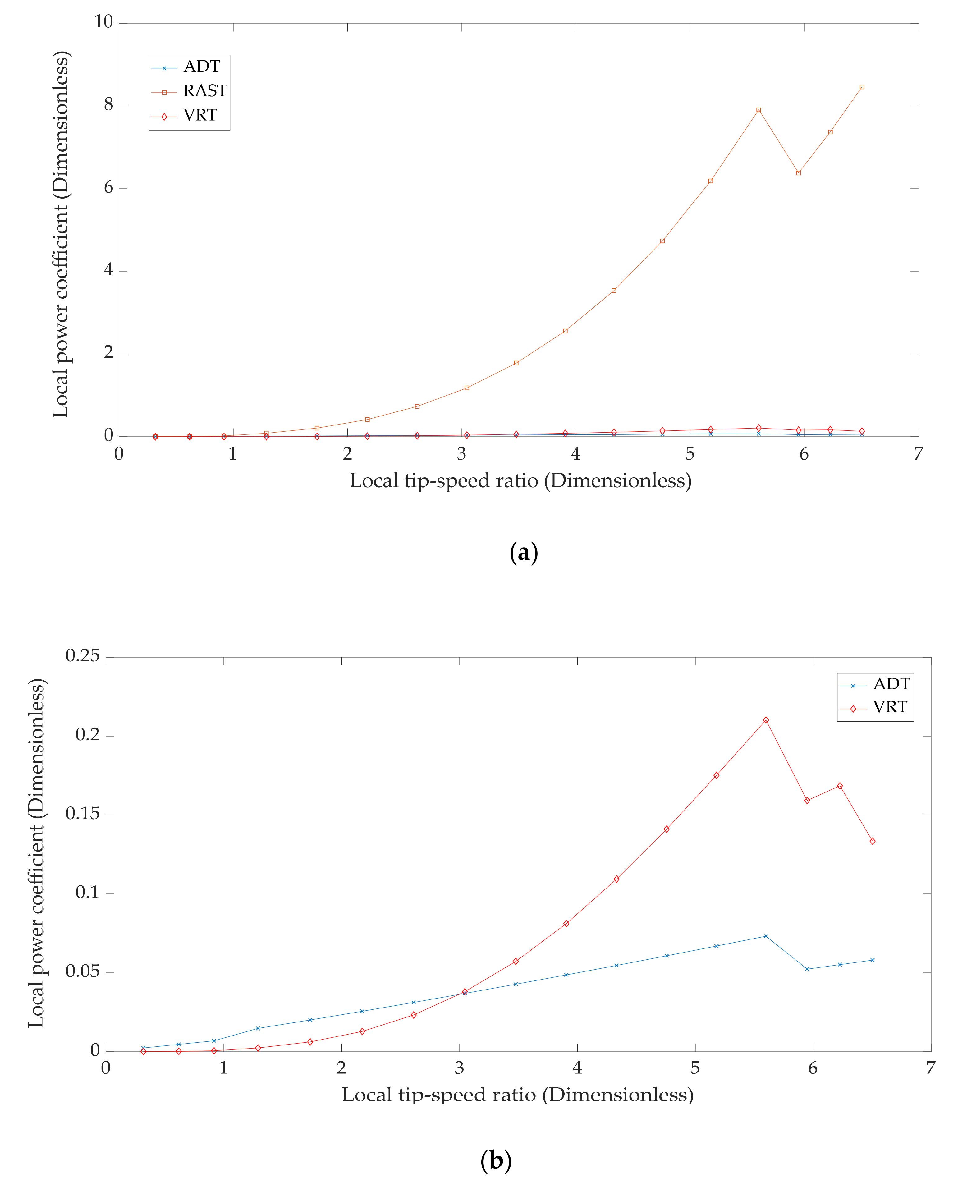
The curves of the local power coefficient
dCP as a function of the local tip-speed ratio
λ(
r) for the ADT, the RAST and the VRT are shown in
Figure 7a. For clarity, the plot of the local power coefficient as a function of the local tip-speed ratio is plotted for the ADT and the VRT as depicted in
Figure 7b. The three curves in
Figure 7a appear to coincide at local tip-speed ratios ranging from about 0.32 to 0.918 after which the RAST curve leaves the ADT and VRT curves. Even though the ADT and VRT curves appear to coincide and run parallel to the horizontal axis at local tip-speed ratios between 0.918 and 4.33 as seen in
Figure 7a, the two curves do intersect at local tip-speed ratios of about 0.32 and 2.900, respectively, as seen in
Figure 7b. For local tip-speed ratios between 0.320 and 2.900, the ADT curve runs above the VRT curve because the
dCp values of the former are higher than those of the latter within this range of local tip-speed ratios. After this range of local tip speed-ratios, the VRT curve runs above the ADT curve as depicted in
Figure 7b. The three theories appear to agree for local tip-speed ratios between 0.32 and 0.918, while the ADT and the VRT agree at local tip-speed ratios of 0.32 and 2.900. The RAST curve rises from values of
dCp slightly above zero to about 7.908 for 0.3 ≤
λ(r) ≤ 5.6 with an upward concavity after which it falls steeply to about 6.38 at a
λ(r) of about 6.0 and rises thereafter. The VRT curve follows the same trend as the former within the same range of local tip-speed ratios, with a peak value of
dCp of about 0.21 at
λ(r) ≅ 5.6 and a trough at
dCp ≅ 0.159 and
λ(
r) = 6.0. It then rises to another peak at
λ(
r) = 6.3 and drops thereafter. The ADT curve stays relatively flat for 0.3 ≤
λ(
r) ≤ 5.6, even though this portion of the curve is supposed to have an upward concavity. It then exhibits a gently sloping peak at
dCp ≅ 0.073 and
λ(
r) = 5.6 followed by a drop to a trough at
dCp ≅ 0.052 and
λ(
r) = 6.0 and rises thereafter. It is worth noting that the values obtained from both the ADT and the VRT are low relative to those of the RAST, so much so that the concavity of their curves is adversely affected when plotted together with the curve of the RAST, a consequence of which is the flatness of their curves for 0.3 ≤
λ(
r) ≤ 5.6. Also worthy of note is the fact that
dCp values for the VRT are higher than those estimated from the ADT, while the values estimated using the RAST are higher than those of the former two theories. This disparity in the magnitude of
dCp results from the fact that the RAST considers the local torque to be generated by the wake-induced angular speed on the rotor as stated in Equation (16), whereas the local torque estimated using the VRT results from the pressure difference across the WT rotor as expressed in Equation (64), while the power estimated from the ADT is the result of the product of the axial thrust expressed in Equation (2) and the wind speed at the rotor. The actuator disk and rotating annular stream-tube theories also consider the rotor as a disk.
The best fit curves for all the three theories are third-degree polynomials. The best fit curves are obtained with a 95% confidence interval using the MATLAB plotting tool. The best fit third-degree polynomial obtained for the ADT with a coefficient of determination of 0.9732, resulting in a correlation coefficient of 98.65%, is
After integrating Equation (85) with respect to
λ(
r) within the limits 0 ≤
λ(
r) ≤
λ, the resulting expression is
subject to the following constraints:
and 0.0001104 <
Cp ≤ 0.3102. The optimum
Cp for the HAWT in this study using the ADT is
at
.
The best fit third-degree polynomial obtained for the RAST with a coefficient of determination of 0.9755, resulting in a correlation coefficient of 98.76% is given by
After integrating Equation (87) with respect to
λ(
r) within the limits 0.155 ≤
λ(
r) ≤
λ, the resulting expression is
subject to the following constraints: 2.2 ≤
λ ≤ 2.973 and
. The optimum
Cp for the HAWT in this study using the RAST is
at
λ = 2.973. Typically, wind farms are designed based on
, and this value is achieved at
λ = 2.746 in the case of the RAST.
A best fit third-degree polynomial with a coefficient of determination of 0.952, resulting in a correlation coefficient of 97.57%, is obtained for the VRT using the MATLAB curve fitting tool:
After integrating Equation (89) with respect to
λ(
r) within the limits 0.155 ≤
λ(
r) ≤
λ, the resulting expression is
subject to the following constraints: 1.6 ≤
λ ≤ 7.572, 8.7 ≤
λ ≤ 10.4 and 0.00022 <
CP ≤ 0.593. The optimum
Cp for the HAWT in this study using the VRT is
at
λ = 7.572 and
λ = 8.700. The typical design
is obtained at
λ = 5.777 in the case of the VRT. It is worth noting that the axial induction coefficient due to the wake and solidity are equal in the cases of the RAST and the ADT, whereas the VRT uses different values for the axial induction coefficients due to the wake and solidity of the WT rotor. An axial induction coefficient of
as(r) = a(r)= 0.293 is used in this work, while the VRT uses a range of axial induction coefficients due to the wake of the rotor within 0.0201 ≤
aw(r) ≤ 0.2566, resulting in 0.3129 ≤
δ(
r) ≤ 0.5493. It can be inferred from the foregoing that the ADT is suitable for the analysis of WTs with high tip-speed ratios, whereas the RAST and the VRT are suitable for WTs with low tip-speed ratios. Typically, smaller WTs have higher tip-speed ratios than larger WTs, such as OWTs.
Figure 8 depicts the plot of the thrust coefficient per unit span
dCT/dr as a function of the local radius
r for the vortex ring, rotating annular stream-tube and actuator disk theories. The VRT curve is seen to run almost parallel to the horizontal axis from
dCT/dr ≅ 0.00026 at
r = 2.8667 m to a peak at
dCT/dr ≅ 0.00219 and
r = 59 m and drops to
dCT/dr ≅ 0.0016 at
r = 61.633 m. It is worth noting that despite the apparent flatness of the VRT curve, it has an upward concavity for local radii between 2.8667 m and 59 m. The ADT and RAST curves merge at all local radii. This merger is the upshot of the equality in the numerical values of
dCT/dr obtained from respective expressions for these theories. Despite the apparent cubic dependence of
dCT/dr in the case of the RAST on
r and the linear dependence of
dCT/dr on
r in the case of the ADT, both curves are linear and coincident, thus signifying a complete agreement of these two theories within this range of local radii. Equations (12) and (18) show the dependence of
dCT/dr on
r for these two theories. The coincident curves rise linearly from
dCT/dr ≅ 0.0046 at
r = 2.8667 m to
dCT/dr ≅ 0.1097 at
r = 61.633 m. It is discernible from
Figure 8 that the thrust coefficients estimated from both the actuator disk and rotating annular stream-tube theories are higher than those obtained from the VRT at all the local radii considered in this paper. This difference between the VRT and the other two theories is evident because the latter two theories use the entire cross-sectional area of the path swept by the rotor blades in estimating
dCT/dr, whereas the VRT uses the planform area of each rotor blade to estimate
dCT/dr. It can also be discerned from
Figure 8 that the load on the WT rotor is linear as exhibited by the ADT and RAST curves, whereas the VRT curve shows that the load on the WT rotor blades is nonlinear.
Worthy of note is the fact that both the actuator disk and rotating annular stream-tube theories assume that the static pressure resulting from the pressure difference across the rotor acts in the axial direction with no component acting in the tangential direction. If this were the case, then there would be no rotation on the WT rotor unless there was another source of rotation coupled with the WT. This assertion that the entire static pressure extracted from the wind by the WT acts in the axial direction and is converted to the axial thrust defies the laws of mechanics because for there to be a rotation of the WT rotor, there must be a tangential component of the resultant force. Based on the foregoing, the actuator disk and rotating annular stream-tube theories are only suitable for the analysis of propellers and not WTs. On the contrary, the VRT is more suitable for WT analysis because it accounts for the tangential component of the static pressure in its initial formulation.
Comparison of the VRT Results to Existing Numerical and Experimental Results
Based on the results depicted in Figure 13 in Reference [
28], the following data were estimated from the cited figure for a blockage ratio of 0.2 and laminar inflow conditions. The results of the numerical analysis and the experiment are shown in
Table 2. The data in
Table 2 are plotted on the same plot as those from Equations (85), (87) and (89)—the expressions for the power coefficient obtained from the three theories and the resulting plots are shown in
Figure 9. It is discernible from
Figure 9 that both the curves of the vortex ring and actuator disk theories follow the same trend as both the existing numerical and experimental curves, even though for tip-speed ratios between 1.6 and about 6.5, the experimental values are higher than those of the VRT, while for tip-speed ratios between 1.6 and about 7.8, the numerical values are higher than those of the VRT. For tip-speed ratios between 1.6 and about 3, both the numerical and experimental curves nearly coincide after which the experimental curve leaves the numerical curve and runs above it up to a tip-speed ratio of about 4.3 and then runs below the numerical curve thereafter. For tip-speed ratios between about 7.8 and 8.5, the VRT curve runs above the numerical curve, while it runs above the experimental curve for tip-speed ratios between 6.5 and 10.2.
Beyond these limits of tip speed ratios, both the experimental and numerical curves run above the VRT curve. The VRT curve intersects with the experimental curve at tip-speed ratios of about 6.5 and 10.2, while it intersects with the numerical curve at tip-speed ratios of about 7.8 and 8.5. It is discernible from the plot that the RAST curve, even though a fourth-degree polynomial like the rest of the curves, is not valid for tip-speed ratios greater than 2.973 because beyond this limit, the power coefficients estimated from the RAST are greater than 0.593 in most cases; beyond this limit, they are greater than unity. On the contrary, both the curves of the vortex ring and actuator disk theories have upward concavity like the numerical and experimental curves. The values of the power coefficient estimated from the ADT are higher than those of the VRT at tip-speed ratios between 1.6 and 4, with both curves intersecting at tip-speed ratios of 4 and about 9.7, respectively. At tip-speed ratios between 4 and about 9.7, the values of the VRT are higher than those of the ADT, while the numerical values are higher than those of the ADT at all the tip-speed ratios considered. At tip-speed ratios greater than 9.7, the values of the power coefficient estimated from the ADT are higher than those of the VRT. It is worth noting that at tip-speed ratios below 2.2, the RAST curve shows negative values of the power coefficient, while at tip-speed ratios beyond 10.4, the VRT curve shows negative values of the power coefficient, and the experimental curve shows negative values of the power coefficient at a tip-speed ratio of 11.2 and beyond. Clearly, among the three theories, the VRT is the most reliable since the values predicted from the VRT lie between the numerical and experimental values and between the values predicted from the ADT and the experimental values within the range of tip-speed ratios at which the VRT is valid. Suffice it to say that the predictions of the VRT agree with the numerical and experimental results at the points of intersection of the curves.


