Abstract
With the recent advent of technology within the smart grid, many conventional concepts of power systems have undergone drastic changes. Owing to technological developments, even small customers can monitor their energy consumption and schedule household applications with the utilization of smart meters and mobile devices. In this paper, we address the power set-point tracking problem for an aggregator that participates in a real-time ancillary program. Fast communication of data and control signal is possible, and the end-user side can exploit the provided signals through demand response programs benefiting both customers and the power grid. However, the existing optimization approaches rely on heavy computation and future parameter predictions, making them ineffective regarding real-time decision-making. As an alternative to the fixed control rules and offline optimization models, we propose the use of an online optimization decision-making framework for the power set-point tracking problem. For the introduced decision-making framework, two types of online algorithms are investigated with and without projections. The former is based on the standard online gradient descent (OGD) algorithm, while the latter is based on the Online Frank–Wolfe (OFW) algorithm. The results demonstrated that both algorithms could achieve sub-linear regret where the OGD approach reached approximately 2.4-times lower average losses. However, the OFW-based demand response algorithm performed up to twenty-nine percent faster when the number of loads increased for each round of optimization.
1. Introduction
In recent years, the improvement of communication technology and the evolving concept of smart grids has enabled new capabilities, such as the activation of demand with demand response (DR) in power systems [1,2,3,4,5]. A study [1] reviewed the technologies developed within the concept of a smart grid to provide DR capabilities. For instance, smart meters, automated meter readings, communication units, monitoring, and control technology equipment are addressed in this work thoroughly. In [2], other related technology, especially storage technologies, are investigated to provide the types that could more effectively activate the demand side for various kinds of DR programs.
This was also analyzed in [3] but for a more specific case of electric vehicles. A special case of DR is for the emergency cases and electricity outages within the grid, which is explored in [4] within the concept of the smart distribution grids, and the required infrastructure and a management model are explained in this regard. Optimization aspects are considered in [5] where loads are presented to the electricity market within a virtual power plant. In this work, it was demonstrated how different sources of uncertainty coming from renewables and demand response can be handled to achieve proper profits.
Even though the notable ability of load activation is known to benefit all participants within the grid, a new challenge is presented: How to make an optimal decision within the limited time that DR signals are provided [6,7]. In the previously existing optimization solution frameworks, the issue of computational time was not properly considered as, normally, decisions are made some time prior to the real-time implementation.
However, this is not the case for DR, especially where the residential loads are engaged. The decision-making intervals depending on the type of DR program could be reduced to seconds. Clearly, utilizing the existing approaches that rely on the high-computational demand and future prediction becomes almost impossible to implement since the optimization period and also computational capability is very limited, and there are several loads where the signals need to be read in time [8,9].
The limitation mentioned above, which comes from the requirements to have rapid yet competent decisions with limited information, necessitates a specific framework: online decision-making. In the context of online decision-making, the whole horizon of the decision-making is divided into small intervals for which separate data of uncertain parameters are available and for each interval value of decision variables are needed to be decided consequently [10].
Indeed, when optimization time is limited, in many practical cases, the procedure of decision-making can become complex, and, as a result, devising a complete model and employing existing classical optimization algorithms will not be possible [11,12]. Online optimization-based methods deal with these deficiencies by implementing online algorithms that incorporate learning from experience and feedback as optimization proceeds and are already popular in control science and applications, such as communication networks and the internet of things [13,14]. Recently, these algorithms have been investigated in power systems and DR contexts as well [15,16,17,18,19,20]. Note that another way to deal with such problems is to utilize deterministic artificial intelligence-based approaches [21]. However, considering the setting of our problem, the focus is on the first option in this study.
Optimal frequency control was addressed in [15]. An online optimization framework was defined and utilized in order to extract an online policy that can react on time when required in the frequency control optimization problem. The proposed control policy has a threshold structure and achieves sub-optimal, however, efficient performance regarding a lack of data about future uncertain parameters. The authors in [16] investigated voltage regulation problems for the electric distribution systems implementations, and the utilized model incorporated online optimizations regarding the structure of the decision-making. In [17,18], the authors studied the online decision-making framework to set pricing stratagems for DR programs.
In [17], online pricing was proposed for DR programs. It was assumed that a utility company was in charge of N users and communicated with them only through a price signal. The user response is known afterward, and no negotiation was considered, meaning that there was only one round of optimization at each time step. This assumption makes sense as, in real-time, considering the communication delay, the time for the required optimizations is very limited.
An online algorithm was proposed in this work that utilized the concept of regret for learning and as a performance metric. Regret is a common term in online optimization and is frequently used to determine the performance of an online algorithm. The regret is greater than zero and is dependent on the algorithm performance and the process of updating the decision of the next step. A good algorithm should achieve a sub-linear regret, or in other words, when the time increases, the average regret should tend to zero.
Study [18] aimed to utilize online learning while designing a load scheduling learning (LSE) algorithm for multi-residential users participating in a real-time price-based DR program. In this study, the focus was on the long-term instead of users who aimed to minimize their cost in a short-term period (i.e., a day). In doing so, the interaction among the users could change the overall consumption and, as a result, the pricing schemes made by the utility within the demand response program. The DR program was considered to be price incentive-based, where prices are generally IBR-based but can also change over time.
Several assumptions were considered regarding the prices and users’ behavior, mainly to shift the problem and reassert it as a Markov decision process and guarantee that the Markov perfect equilibrium exists. In addition, it was presumed that the price parameters were generated according to a hidden Markov model. With this assumption, it was demonstrated how to estimate the necessary action probabilities and profile observation. Finally, the authors proposed a model including the interactions among users and the utility leading to the decreased cost values in the long-term run, where they considered the sequential decision in the process.
Studies [19,20] have designed online algorithms to solve decision-making issues for the online optimization of an end-user customer participating in a real-time pricing DR program. In [19], an algorithm was proposed in which the decision was updated regarding the gradient of the cost function. The demand response model utilized as the base case for the study was the one presented in [22]. They demonstrated that, through a day, the proposed online algorithm could perform satisfactorily compared to the existing approaches that utilized an offline approach combined with the rolling window concept [22].
This work was extended in [20], and two online algorithms were proposed based on the receding horizon concept that incorporates a very limited window of prediction in the online algorithm. It was demonstrated that these algorithms could perform better than the rolling-window robust optimization approach, and the acquired results were achieved only in seconds where the offline method requires minutes to solve the optimization.
For the residential section, due to a lack of heavy computation capability, the necessity to adapt to multiple fast signals from markets and household appliances makes online decision-making more attractive. The available literature lacks in terms of investigating the capability of online decision-making to provide residential consumers with daily consumption optimization within known DR programs, such as set-point tracking problems.
In this study, we investigate a set-point tracking problem utilizing DR at the residential level. We consider an aggregator that is in charge of a large population of thermostatically controllable loads (TCLs) that, by increasing or decreasing their consumption at each step, attempts to track the reference signal. The general decision-making framework is that a decision is made without relying on any prediction and information about future parameters. Thus, the aggregator decides the increase or decrease in consumption of each load at time t. After committing to a decision, the signal to be tracked and the uncertain response of each load is realized; therefore, the aggregator suffers a loss, and decisions can be updated accordingly.
These decisions are required to be made fast. Consequently, in this work, two types of online algorithms based on classical optimization algorithms are modified and applied to the aforementioned problem, namely online gradient descent (OGD) and online Frank–Wolfe (OFW). The first involves a projection at each step, and the second is a projection-free algorithm. In this work, the aim is to investigate not only the general performance in terms of the loss function optimization but also the computational time and burden. As mentioned above, in this set of real-world problems, the solution needs to be found within seconds otherwise those approaches, even with a good general performance, become impotent.
In summary, the contributions of this study are as follows:
- (1)
- We propose two algorithms to address autonomous decision-making for the set-point tracking problem of residential TCLs. The offered approaches are easy to implement for the residential end-users and could output decisions very fast, thus, matching the required real-time settings.
- (2)
- We analyze and evaluate the aptitudes of the proposed algorithms while giving a fully comparative set of numerical studies.
The remainder of the paper is organized as follows. Section 2 explains the mathematical framework and the structure of each online algorithm. The set-point tacking optimization problem is introduced in Section 3. Numerical results are illustrated in Section 5. Finally, Section 7 concludes the paper.
2. Mathematical Framework of Online Decision Making
The online decision-making framework can be simply explained with a brief example. Imagine a merchant having a small section in a flea market. He owns a few items that need to be sold by the end of the day. Customers approach the rented space one by one asking about the cost of the available commodities. A price is provided by the merchant, and they decide whether to purchase anything or not. The objective here should be to maximize the profit by the end of the day. However, there are some insights about the offered prices to the customers, and they cannot be too high or low.
Indeed, if proper valuations are not chosen regarding the customer behavior, the merchant may end up with either unsold goods or all sold-out with low prices leading to an unsatisfying profit. Meaning that considering uncertainty toward the future in terms of coming customers and their will to buy, there is a need to design an algorithm that learns and evolves the pricing strategy each time a new customer wants to buy a commodity.
The aforementioned situation depicts an online decision-making problem that is also shown in Figure 1. Indeed, through the day, the merchant learns and evolves the decision-making to maximize the total profit. Formally and with mathematical notation an online decision-making problem is given in Figure 2.
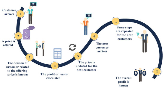
Figure 1.
Online decision-making framework for flea-market merchandise [20].
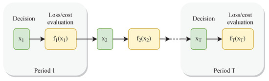
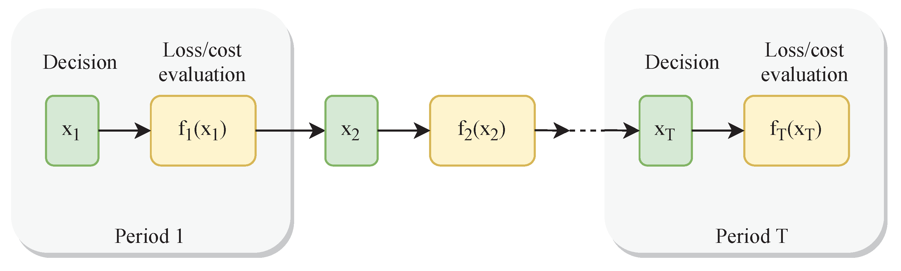
Figure 2.
Online optimization decision-making framework.
When online optimization is considered, decision-making is conducted in a limited number of consecutive rounds. At each round, the optimization variables are decided without relying on future information. After assigning specific values to the decision variables, the uncertain parameters are realized. Based on the new information (i.e., a loss function), the previous round’s performance can be measured, and the decision for the next round can be updated accordingly.
In a classical optimization setting, since only one objective function exists, the goal is to minimize this function. For instance, the utilization of iterative algorithms and their performance is measured by the convergence rate, which shows whether they could converge to the optimal point. A linear convergence is a favorable one in the context. However, in the online optimization setting, at each interval, a new function is observed. Thus, a new performance measured is defined in this setting that is called dynamic regret, , which is the difference between the accumulation of instantaneous cost and the best performance at each period [23], as depicted in (1).
Here, is the cost function at time period t, T is the final time period, is the decision made by the online algorithm, and is the best decision at time t. An online algorithm performance is measured by regret, and a good online algorithm should achieve sub-linear regret meaning that the average regret would tend to zero when the number of rounds increases. Note that, if the loss function f and the decision-making set are convex, the online decision-making optimization is called online convex optimization (OCO) [24].
A well-known online algorithm is called online gradient descent and was first introduced in [25]. There are several algorithms developed based on the OGD and applied to many problems in theory and practice [26,27]. The OGD is given in Algorithm 1.
In this algorithm, the input parameters are , which are similar to other values of decision belonging to the decision-set . Parameter is the step-size and is assumed to be a fixed value through the whole process of decision-making. The algorithm utilizes gradient descent with the step size of at each step after observing . However, this value is required to be in the bound defined by the decision-making set. Therefore, a projection step is performed in each step as well.
The OGD-based algorithms are widespread and typically very efficient; however, as explained above, they rely on a projection step whenever a decision is taken outside the domain of interest (i.e., the infeasible decision value), which can limit their potential in multiple applications. The projection step indicates obtaining the closest point inside the decision-making set and could require solving a convex quadratic program each time the optimization variable is decided.
In many settings of practical interest, linear optimization can be carried out more efficiently. In this avenue, another type of online algorithm is proposed based on the Frank–Wolfe algorithm, which does not require projection at any step and is also very easy to implement. In the context of the Frank–Wolfe approach, it is assumed that the linear optimization step is computationally cheap compared to the projection counterpart. The linear programming optimization in some applications can simplify the implementation of the whole optimization as well. The online Frank–Wolfe optimization is given in Algorithm 2 [28].
| Algorithm 1: OGD Algorithm |
| Inputs, for to T do Use and observe Compute: = Project: = end |
| Algorithm 2: OFW Algorithm |
| Inputs, for to T do Use and observe Compute gradient estimate: = Compute: Set: end |
3. Set-Point Tracking Modeling
Electric utilities, along with power system operators, consider DR as a practical tool to activate the demand side to participate in grid functions when necessary. When utilized appropriately, demand response could prove to be an economical and sustainable solution benefiting both customers and grids simultaneously.
DR can have different attributes, including the DR duration, frequency, and response time. Indeed, the practical implementation of DR could take different time scales, automatizing levels, and response size. For instance, large demand loads can be called by phone by system operators hours before an event of DR (the frequency is low). Opposite to large loads, we have small appliances that are faster, and the frequency is higher but would need to respond autonomously, with small intervals for updating their response (ranging from seconds to a few minutes and a higher frequency of DR). Here, we investigate set-point tracking that requires fast responses from the engaged load in the DR program.
We assume an aggregator (central utility) managing certain types of residential appliances that provide ancillary services to the power grid. A regulation signal [29] is received by the aggregator, and the task is to convert this signal into the state decisions of the individual TCLs. Therefore, for each TCL, an adjustment signal is provided at each optimization interval to track a power set-point via the aggregated consumption. Each household appliances’ energy consumption is managed by an EMS installed in the customer’s home, which receives online control signals from the aggregator.
We consider N flexible loads in the order of hundreds or thousands. The decision variables are the amount of adjustment at each interval, which translates into . Thus, at each time, the loads can be adjusted to match the set-point signal . We assumed that the response of the loads is under uncertainty. In this regard, the following loss function is chosen to penalize the large deviation from the set-point signal:
Here, is the loss function, and represents the uncertainty of the load behavior.
The responsive loads are considered to be TCLs. We assume the cooling phase (air condition); however, the model can be extended for heating. From [28], the temperature evolution of a TCL can be represented as follows:
Here, is the TCL i internal temperature at interval t, where R and C are the thermal resistance and capacitance, respectively, is the ambient temperature, is the control variable, and finally . We adopt the model so that the energy level can be changed in a continuous range, and this way the acquired temperature can be achieved easier. In addition, this complies more with the structure of the state of art TCLs found in residential departments.
We assumed that the air conditioner is working to give the desired temperature; thus, at each interval that TCL is participating in DR, this temperature may be increased or decreased depending on the control signal provided by the central operator, which, in this case, is the aggregator. Thus, the aforementioned loss function is rewritten as given in (4) to be utilized in the online algorithms introduced in the next subsection.
where and .
4. Solution Methodology
The previous section presented the set-point tracking problem and prepared the optimization model to be utilized within an online decision-making framework. Here, we give two online algorithms based on the OGD and OFW algorithms. The OGD algorithm acts a the benchmark and represents the online algorithms that require the projections at each step. Opposed to this, we introduce the OFW-based algorithm that utilizes the linear approximation to solve an LP problem at each stage without the utilization of any projections. Both of these algorithms are introduced in Algorithms 3 and 4.
| Algorithm 3: OGD-Based Set-Point Tracking Algorithm at Time t |
| Inputs, a,, , , Define Decision-making set Begin: Utilize the decision made in the previous time interval: Realize uncertain parameters: , Compute the loss function input parameter: Calculate the loss function: Compute: Project and Update: = End Output: |
| Algorithm 4: OFW-Based Set-Point Tracking Algorithm at Time t |
| Inputs, a,, , , Begin:; Utilize the decision made in the previous time interval: Realize uncertain parameters: , Compute the loss function input parameter: Calculate the loss function: Compute: Compute LP optimization parameters: and according to the decision-making set Solve LP optimization and calculate solution as accordingly Update = End Output: |
The algorithm given in Algorithm 3 represents the process of deciding the next step for TCL operation at time t. There are some input parameters that are known prior to the start of the optimization interval. These parameters include the decision made in the previous time interval, the TCL parameters, the step size, and the desired temperatures.
At the start of the time step t, the , which is set in the previous step, is utilized, and the related uncertain parameters are realized afterward. The loss function could be calculated accordingly. After receiving the complete observation of the loss function, the first stage of updating step is calculated as demonstrated in the algorithm. The result could be outside of the decision-making set. Thus, the final decision is updated and outputted after one projection, which is translated as solving a quadratic program with constraints that define the decision-making set.
In Algorithm 4, similar steps are taken in the first part of the procedure regarding the input, realization, and calculation of the loss function. After computing the loss function, the direction variable is calculated accordingly, which is then utilized in solving the given LP problem in (5).
Here, is determined by the direction variable, the decision-making set boundaries are translated into matrices, and the lower and upper bound are already known from the TCL data. The solution of this LP problem is utilized in the next step to determine the value of . Finally, along with are outputted to be used in the next optimization interval. In the next section, we fully investigate and compare the performances of these algorithms and provide hindsight on how to use them in similar decision-making problems to their full potential.
5. Numerical Study
In this numerical study, we present three different cases:
- Case I:
- In this case, we assume that the fluctuation of set-point tracking is small and that there is no complicating constraint that defines the feasibility set for decision-making.
- Case II:
- In this case, the set-point signal fluctuation range is higher, which makes the tracking more difficult and less predictable.
- Case III:
- Finally, in this case, not only is the fluctuation high but also there are constraints that further complicate the decision-making set.
The numerical experiments wer performed in Python, and CVXP solvers were utilized where necessary to solve the optimization problems (linear and quadratic optimization problems).
5.1. Case I
For this case, we assumed that and , a truncated Gaussian variable, models the TCLs’ response uncertainty at each optimization interval. This uncertainty is related to the limitation of temperature modeling, for instance, the impact of the radiant house heating from the sun or windows being open, etc.
The TCL parameters are sampled uniformly from the thermal parameters depicted in Table 1, and the desired temperature is uniformly sampled in the range of 20 C to 25 C for all loads. The ambient temperature is supposed to be fixed to 30 C considering the fact that the operation time is generally limited, and this temperature, on average, does not vary much. Both OGD and OFW algorithms are applied to the set-point tracking problem as explained in the previous section. The loss function is calculated for the case where , and its evolution is depicted in Figure 3 with a logarithmic y axis in Figure 4.

Table 1.
TCL Parameters.
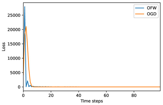
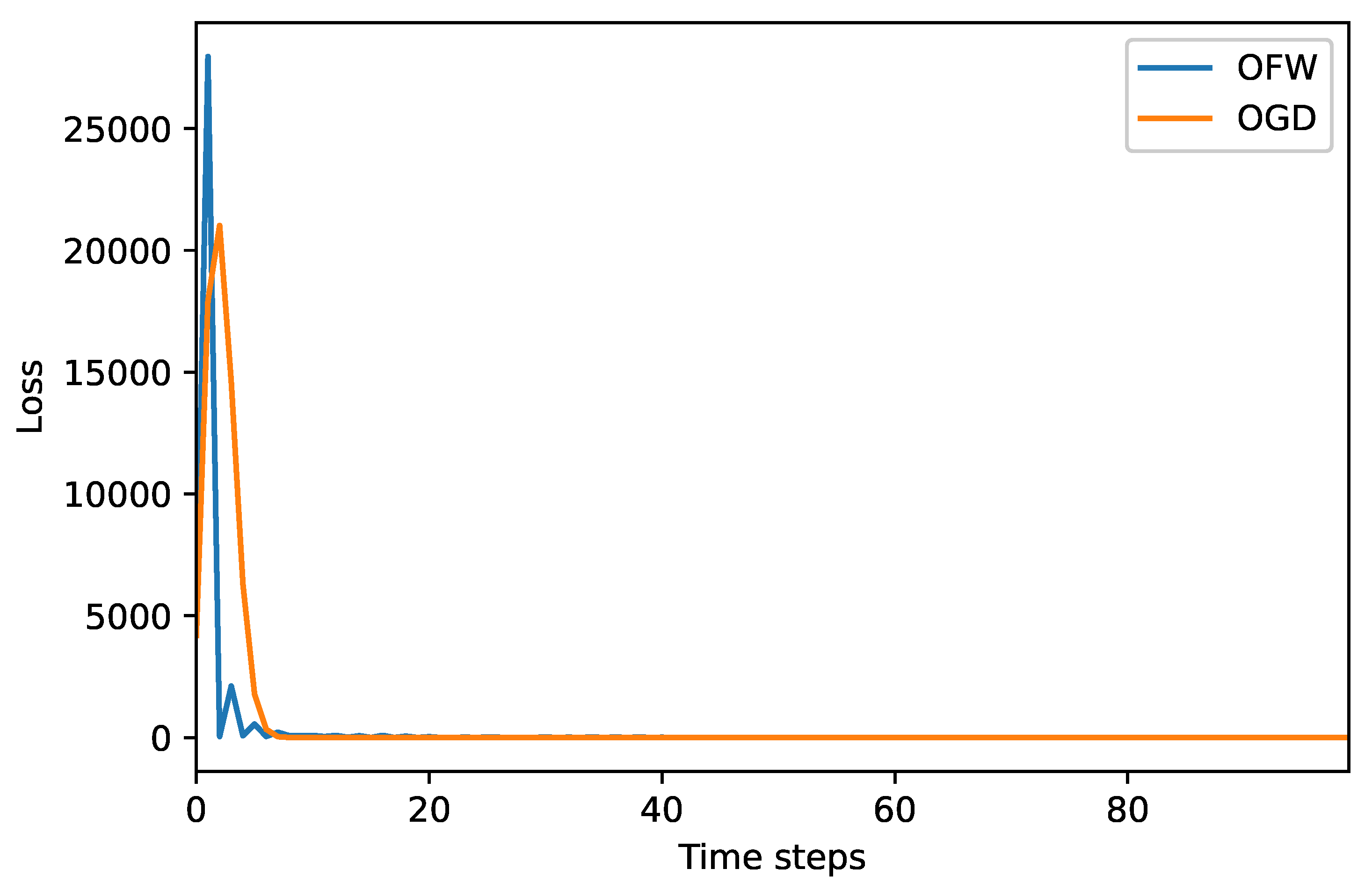
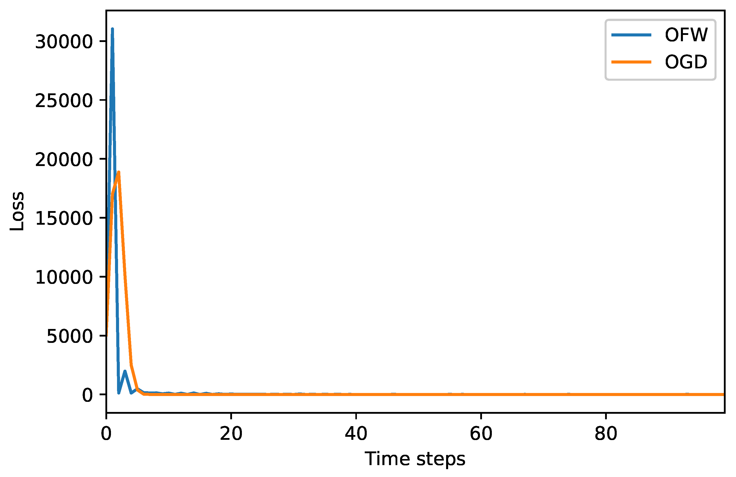
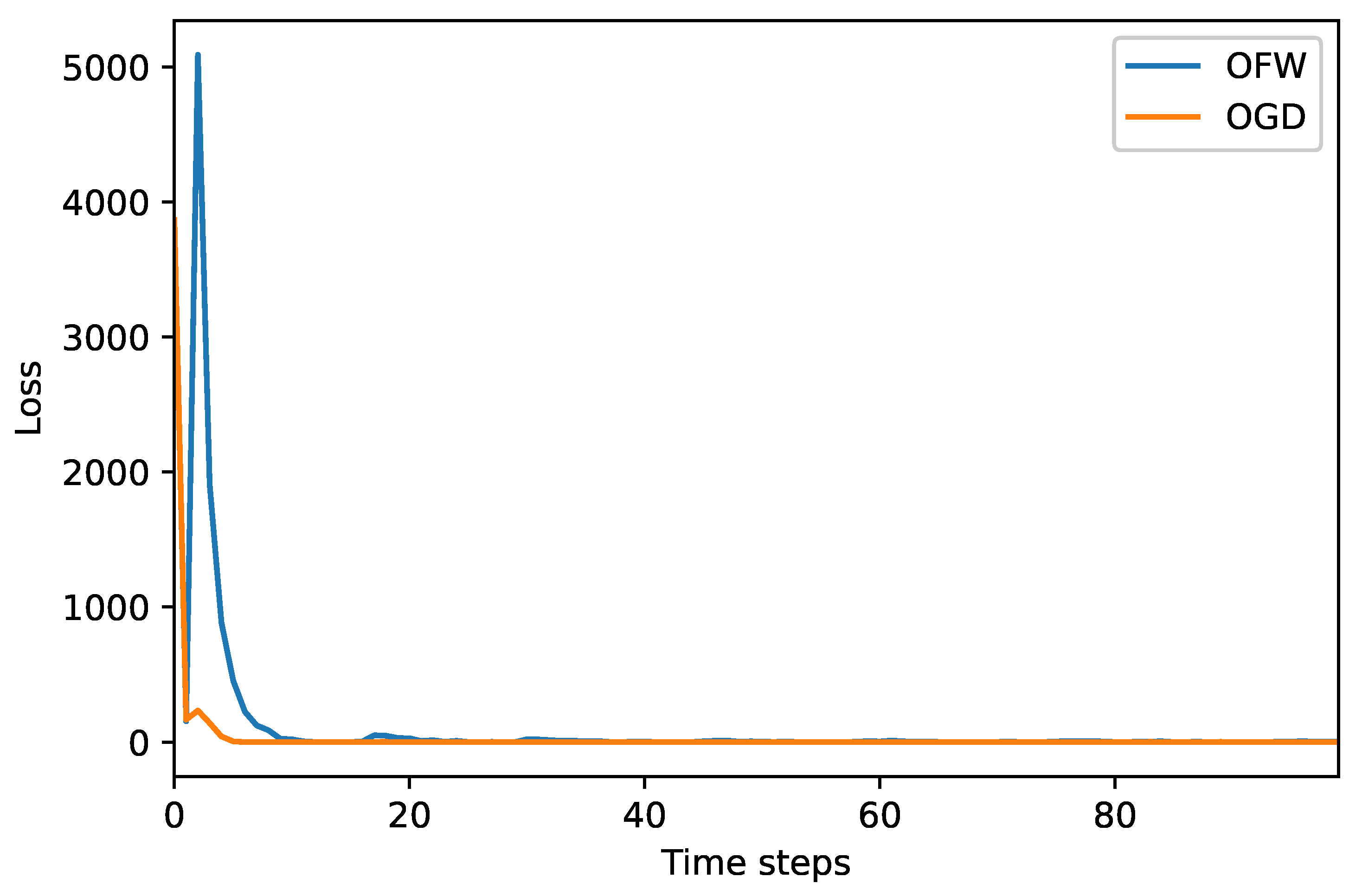
Figure 3.
Comparison of the loss values for each method.
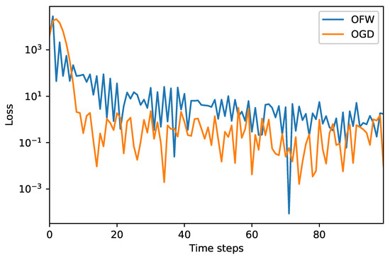
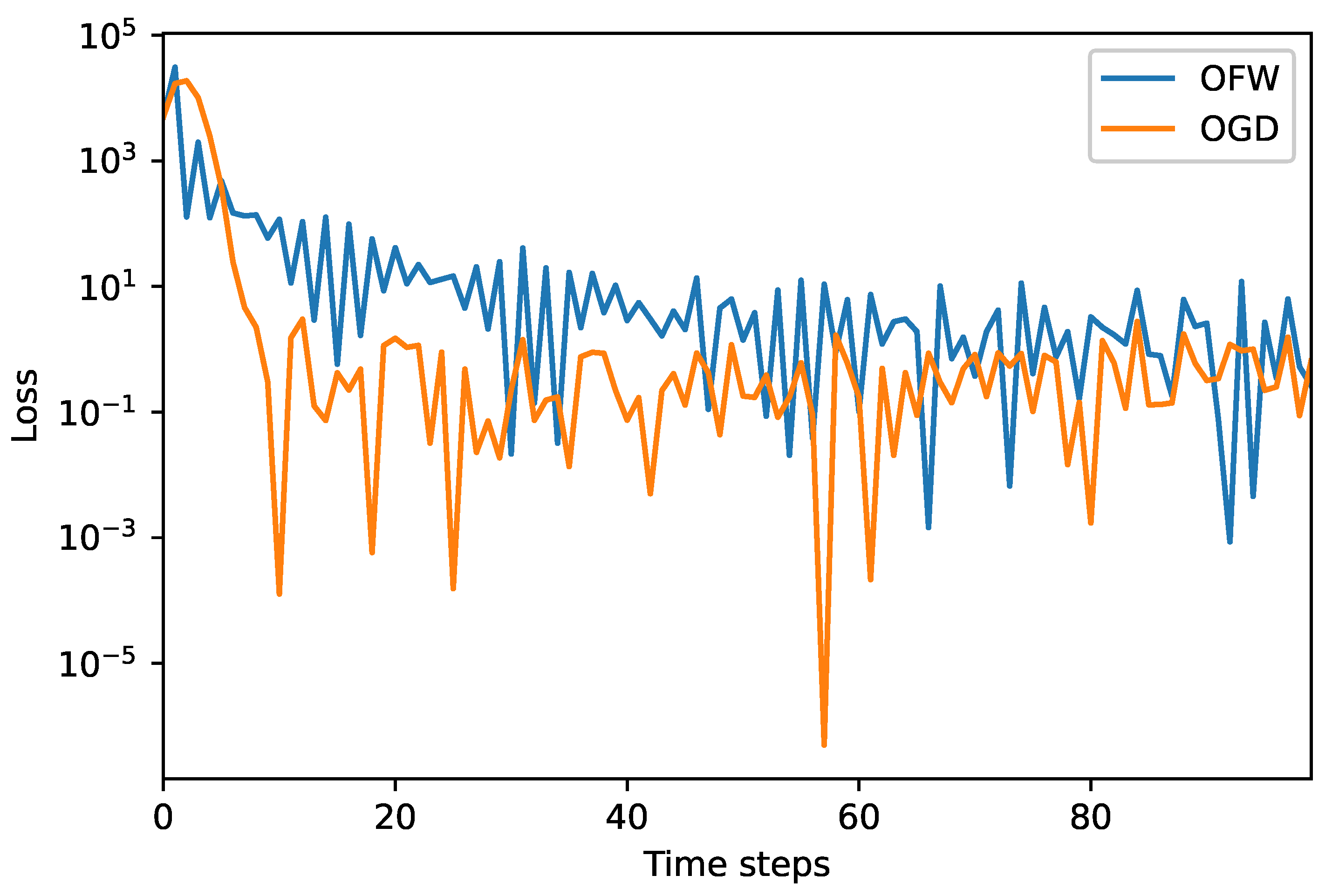
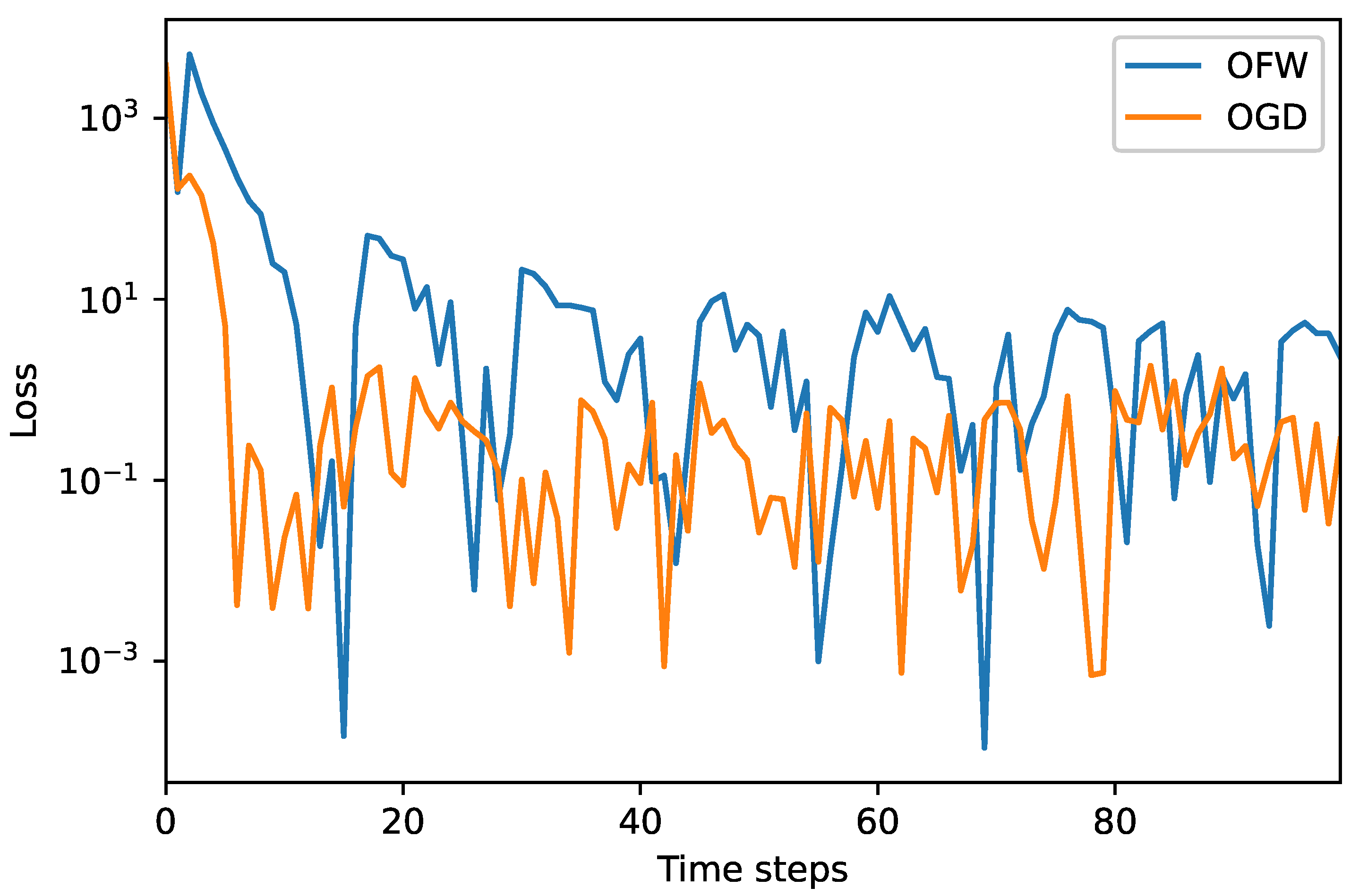
Figure 4.
Comparison of the loss values for each method with a logarithmic y axis.
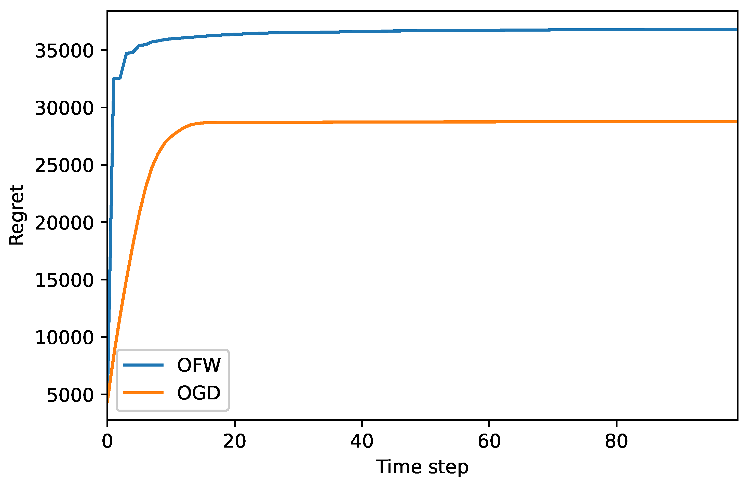
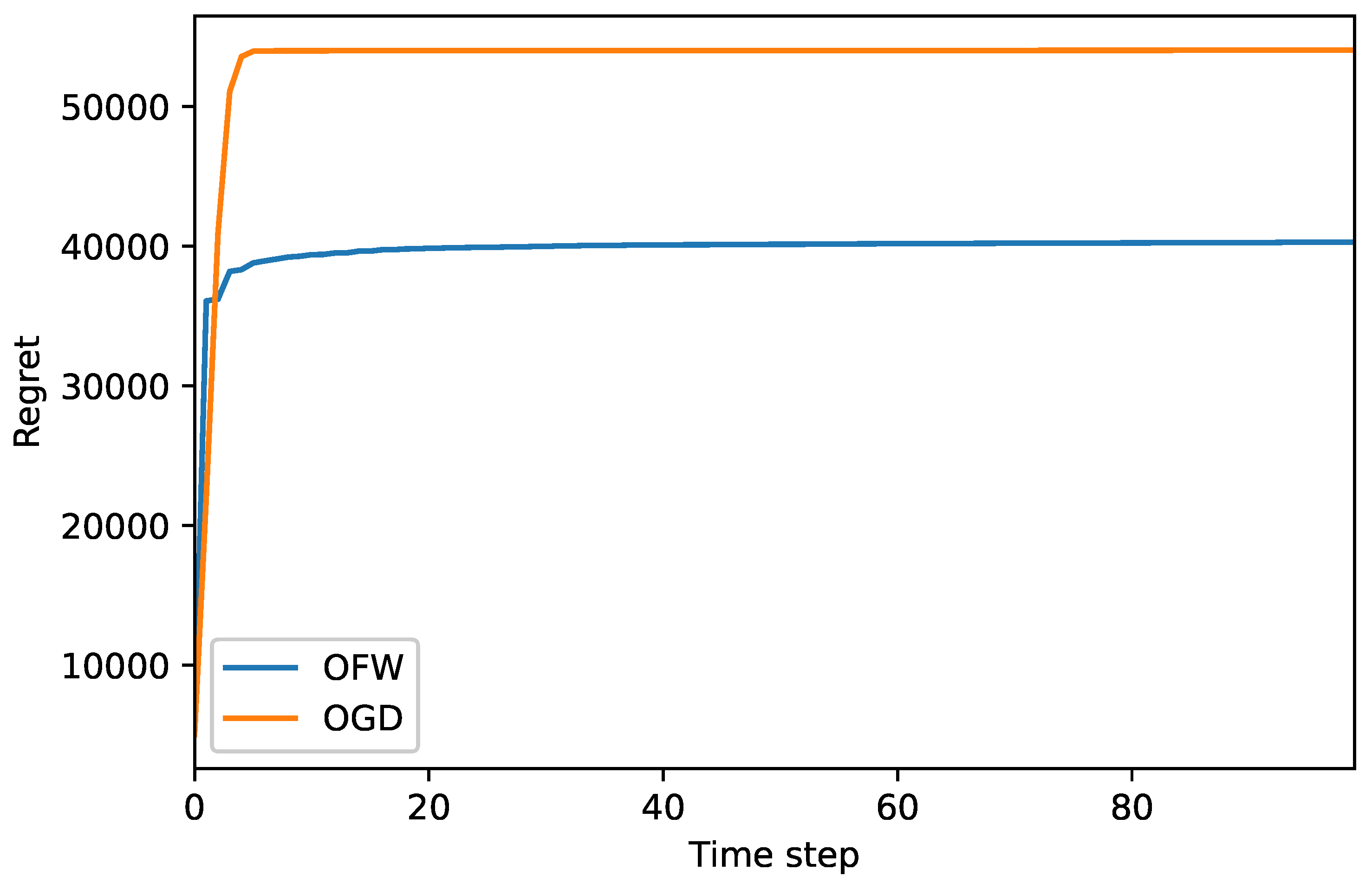
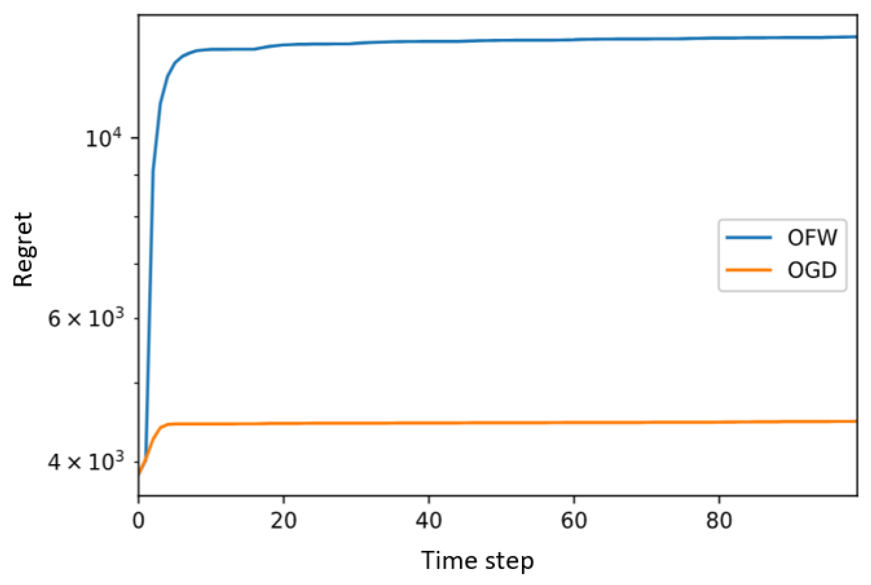
As depicted in these figures, the loss starts to decrease after a few steps of optimization. This decrease is quicker in the OFW case, but both approaches depict a similar behavior where, in some steps, OGD decreases the loss function even further. Next, the regret analysis is conducted in Figure 5. We can see that both algorithms attain a sub-linear regret, which is an important goal when dealing with an online optimization framework, meaning that, when the time increases, the average regret tends to zero or, in other words, online learning is successfully carried out.
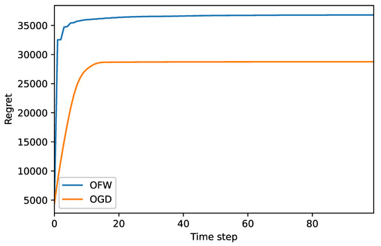
Figure 5.
Regret analysis of both approaches in case I.
5.2. Case II
The only thing that differs in this case is the set-point signal fluctuation size, which is assumed to be defined as . In this case, similar results and sub-linear regret are achieved for both algorithms as shown in Figure 6, Figure 7 and Figure 8.

Figure 6.
Comparison of the loss for both approaches in case II.

Figure 7.
Comparison of the loss for both approaches in case II with a logarithmic y axis.
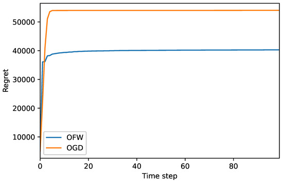
Figure 8.
Regret analysis of both approaches in case II.
It is clear that, despite the tracking signals having a large domain of changes, both approaches can successfully achieve the sub-linear regret in time.
5.3. Case III
In this case, not only is the signal fluctuation range high, in addition, we also assumed that the loads are connected through a transformer that has it is own loading constraints; therefore, the sum of the decision variables is limited, further complicating the feasibility set. The results for the loss function and regret are depicted in Figure 9, Figure 10 and Figure 11. In this case, OGD demonstrates a smoother behavior, and quickly, its loss decays, which results in a better regret behavior. However, after some steps, both algorithms show similar behavior in decreasing the loss and attain a sub-linear regret.
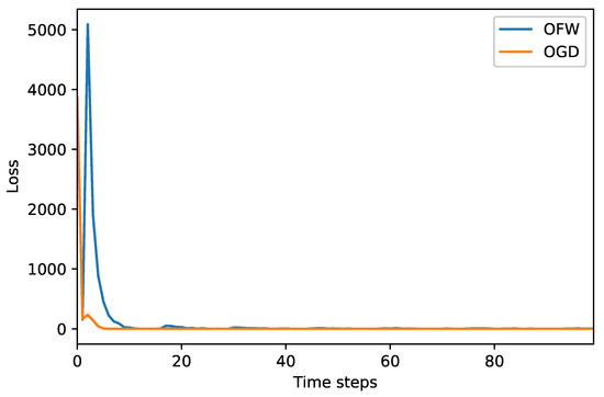
Figure 9.
Comparison of the loss for both approaches in case III.

Figure 10.
Comparison of the loss for both approaches in case III with a logarithmic y axis.
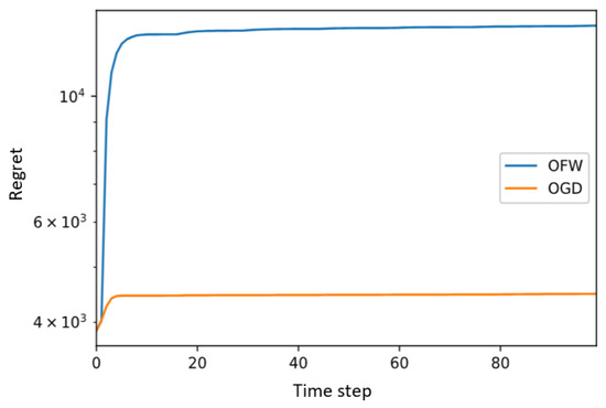
Figure 11.
Regret analysis of both approaches in case III.
6. Discussion
In the previous section, several study cases were presented, and the performance of two algorithms based on OGD and OFW approaches were investigated. It can be seen that, generally, these two algorithms performed satisfactorily in the sense that both achieved sub-linear regret in all three case studies. A more detailed analysis regarding a quantitative comparison in terms of the output of these two algorithms could be found in Table 2. Four different values are given for the three cases acquired by each algorithm. First, the final value of the loss at the end of the optimization period is demonstrated. It can be seen that, in case I, the OGD-based method achieved lower values; specifically, if we calculate the average of all three cases, the OFW loss was 2.24-times higher than for OGD.
Table 2.
Quantitative comparison of different values of the loss achieved by the OGD and OFW algorithms.
This behavior was repeated when evaluating the average loss over the period of 20 to 100 (ignoring the initial fluctuation period), meaning that, for the average loss, OGD could output lower values. However, OFW depicted much better behavior in terms of decreasing the cost in the first five time periods, thus, showing that OFW was faster to approach the targeted signal. Especially in case II, the difference was almost ten-times less for OFW. Finally, OFW reached smaller minimum losses. For instance, the minimum cost reached by OFW was much lower than the OGD counterpart. By calculating the average of the fourth row, it can be seen that OFW achieved a four times lower minimum value compared to OGD. Considering the setting of the optimization problem, the time consumption was also of importance for comparing the performances, which is addressed in the next subsection.
6.1. Scalability Analysis
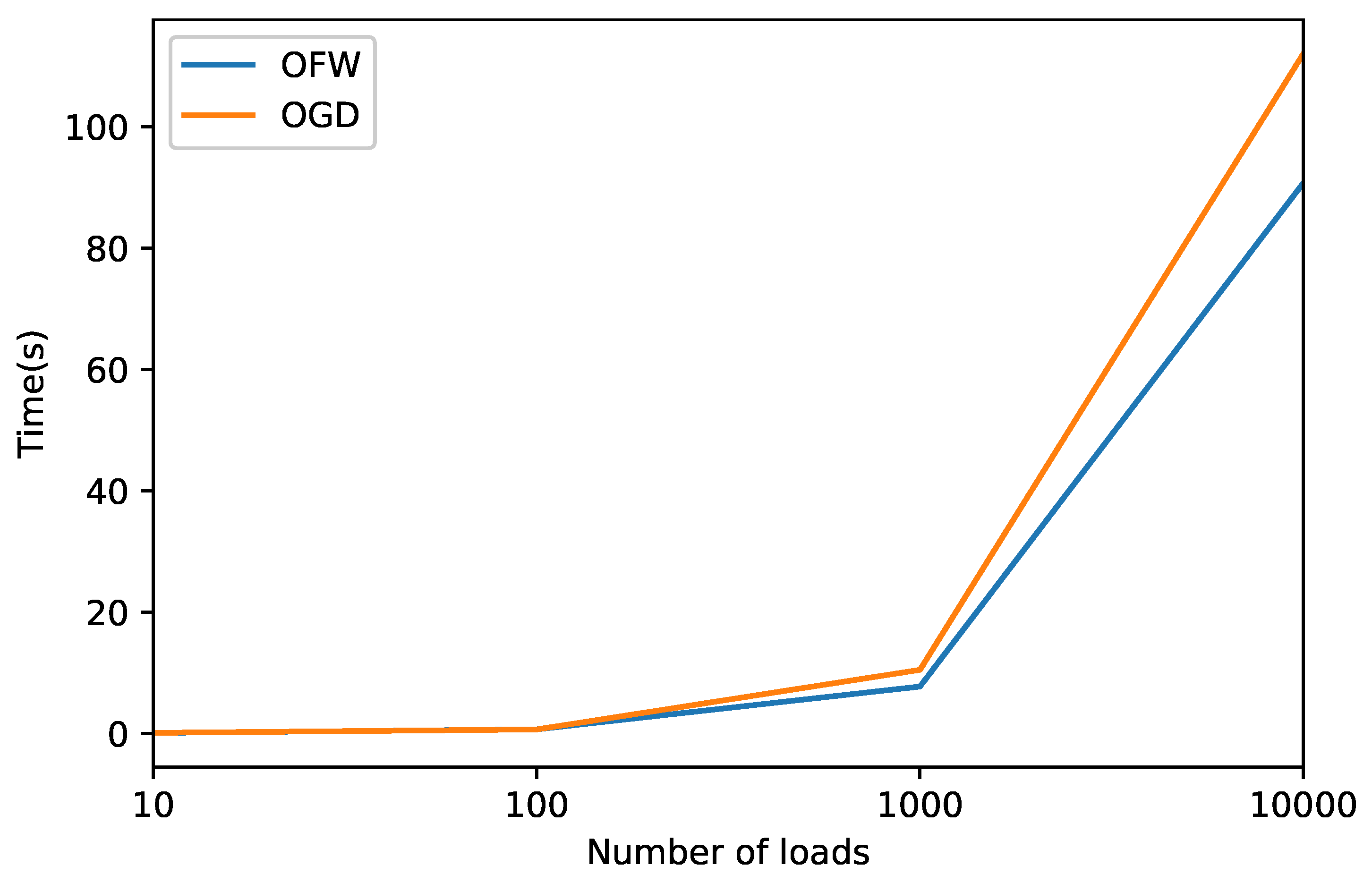
Another important comparison is represented in Figure 12 where, for four different numbers of loads, the time consumption of each approach is measured and demonstrated. Clearly, the OFW approach is the faster one. Especially in the case of 10,000, the difference is more noticeable. In addition, Table 3 gives the time consumption ratio of the two algorithms for better comparison. It can be seen that the OGD algorithm always consumed more time. When the number of loads increased, the difference between the two algorithms was stronger. Especially in the case of 10,000 OGD, the time consumption was twenty-nine percent more. This means that when we are dealing with a large number of controllable loads and we are aiming at utilizing them in a fast ancillary service scheme regarding the delays in the signals, the OFW approach becomes more favorable.
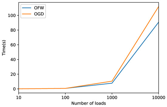
Figure 12.
Comparison of the time consumption of each approach for different numbers of TCLs.
Table 3.
Quantitative comparison of the time consumption with different numbers of loads.
6.2. Implementation Discussion
It is important to note that both algorithms were carried out with theoretically recommended step sizes. However, in practice, better performance can be achieved with specially tuned step sizes for both algorithms. For instance, in the case of OFW, it was always observed that if some warm-start modification step was added to the approach, this could quickly decrease the loss and achieve a very small accumulative loss. Similarly, for the OGD case, some time-varying step sizes could result in better performance; however, this depends on the type of problem and the related parameters. To obtain better insights for the step size tuning, sensitivity analysis is a future extension of this work to construct a warm start modification of OFW and a step-size problem-dependent tuning for the OGD algorithm-based approaches.
7. Conclusions
Evolving technologies make it possible to become more productive while economizing customer energy consumption. This growing suite of technologies includes the possibility to provide market data very fast for demand-side customers, thus, activating them to respond to energy-related signals in a quick fashion.
In this study, the problem of real-time set-point tracking was addressed. In the introduced real-time settings, it was difficult to make fast exact predictions with the popular approaches and even utilizing off-shelf solvers and powerful computing systems still could not produce an optimized solution within the required time (a few seconds). Thus, a decision-making framework based on the online optimization was introduced, and the performances of two candidate approaches (with and without projections) were fully analyzed—namely, OGD and OFW.
We demonstrated that both approaches successfully decreased the loss over time and achieved sub-linear regret, which is the goal of online optimization. Thus, the error of the learning decreased over time and did not increase linearly. In addition, both approaches require further tuning to achieve an ideal performance, which can be a task for future works. The time consumption of both approaches was investigated. As was clearly observed, both algorithms were very fast; however, in applications with more limited time settings, the OFW was preferable.
Author Contributions
Conceptualization, A.A., D.P. and M.F.; methodology, A.A.; software, A.A.; validation, A.A., D.P. and M.F.; formal analysis, A.A., D.P. and M.F.; investigation, A.A., D.P. and M.F.; data curation, A.A.; writing—original draft preparation, A.A.; writing—review and editing, A.A., D.P. and M.F.; visualization, A.A., D.P. and M.F. All authors have read and agreed to the published version of the manuscript.
Funding
This work was prepared as a part of the AMPaC Megagrant project supported by Skoltech and The Ministry of Education and Science of Russian Federation, Grant Agreement No 075-10-2021-067, Grant identification code 000000S707521QJX0002.
Institutional Review Board Statement
Not applicable.
Informed Consent Statement
Not applicable.
Data Availability Statement
Not applicable.
Conflicts of Interest
The authors declare no conflict of interest.
Abbreviations
| Acronyms | |
| EV | Electric vehicle |
| DR | Demand response |
| IBR | Inclining block rates |
| LSE | Load scheduling learning |
| OGD | Online gradient descent |
| OFW | Online Frank–Wolfe |
| TCL | Thermostatically controllable load |
| Sets & parameters | |
| a | Dimensionless TCL parameter |
| C | Thermal capacitance |
| i | TCL index |
| K | Decision-making set |
| N | Number of loads |
| Rated power | |
| R | Thermal resistance |
| Dynamic regret | |
| s | Set-point signal |
| t | Time period |
| T | Number of optimization periods |
| Load response uncertainty | |
| Step size | |
| Efficiency | |
| Ambient temperature | |
| Desired temperature | |
| Temperature gain when TCL is ON | |
| Step size | |
| Step size | |
| Optimization variables | |
| d | Gradient estimate |
| f | Cost function |
| L | Loss function |
| q | Control variable |
| v | Direction parallel to y in the decision set |
| x | Decision variable |
| Best decision | |
| y | Decision value before projection |
| TCL internal temperature | |
References
- Dileep, G. A survey on smart grid technologies and applications. Renew. Energy 2020, 146, 2589–2625. [Google Scholar] [CrossRef]
- Villanueva, D.; Cordeiro, M.; Feijóo, A.; Míguez, E.; Fernández, A. Effects of Adding Batteries in Household Installations: Savings, Efficiency and Emissions. Appl. Sci. 2020, 10, 5891. [Google Scholar] [CrossRef]
- Gharibeh, H.F.; Khiavi, L.M.; Farrokhifar, M.; Alahyari, A.; Pozo, D. Power management of electric vehicle equipped with battery and supercapacitor considering irregular terrain. In Proceedings of the 2019 International Youth Conference on Radio Electronics, Electrical and Power Engineering (REEPE), Moscow, Russia, 14–15 March 2019; pp. 1–5. [Google Scholar]
- Dorahaki, S.; Dashti, R.; Shaker, H.R. Optimal Outage Management Model Considering Emergency Demand Response Programs for a Smart Distribution System. Appl. Sci. 2020, 10, 7406. [Google Scholar] [CrossRef]
- Alahyari, A.; Ehsan, M.; Pozo, D.; Farrokhifar, M. Hybrid uncertainty-based offering strategy for virtual power plants. IET Renew. Power Gener. 2020, 14, 2359–2366. [Google Scholar] [CrossRef]
- Li, H.; Wan, Z.; He, H. Real-time residential demand response. IEEE Trans. Smart Grid 2020, 11, 4144–4154. [Google Scholar] [CrossRef]
- Alahyari, A.; Pozo, D.; Sadri, M.A. Online Energy Management of Electric Vehicle Parking-Lots. In Proceedings of the 2020 International Conference on Smart Energy Systems and Technologies (SEST), Istanbul, Turkey, 7–9 September 2020; pp. 1–6. [Google Scholar]
- Wang, J.; Li, K.J.; Liang, Y.; Javid, Z. Optimization of Multi-Energy Microgrid Operation in the Presence of PV, Heterogeneous Energy Storage and Integrated Demand Response. Appl. Sci. 2021, 11, 1005. [Google Scholar] [CrossRef]
- Farzaneh, H.; Malehmirchegini, L.; Bejan, A.; Afolabi, T.; Mulumba, A.; Daka, P.P. Artificial Intelligence Evolution in Smart Buildings for Energy Efficiency. Appl. Sci. 2021, 11, 763. [Google Scholar] [CrossRef]
- Fan, S.; He, G.; Zhou, X.; Cui, M. Online optimization for networked distributed energy resources with time-coupling constraints. IEEE Trans. Smart Grid 2020, 12, 251–267. [Google Scholar] [CrossRef]
- Bernstein, A.; Dall’Anese, E. Real-time feedback-based optimization of distribution grids: A unified approach. IEEE Trans. Control. Netw. Syst. 2019, 6, 1197–1209. [Google Scholar] [CrossRef] [Green Version]
- Zhong, W.; Xie, K.; Liu, Y.; Yang, C.; Xie, S.; Zhang, Y. Online control and near-optimal algorithm for distributed energy storage sharing in smart grid. IEEE Trans. Smart Grid 2019, 11, 2552–2562. [Google Scholar] [CrossRef]
- Zhang, M.; Zhou, Y.; Quan, W.; Zhu, J.; Zheng, R.; Wu, Q. Online Learning for IoT Optimization: A Frank–Wolfe Adam-Based Algorithm. IEEE Internet Things J. 2020, 7, 8228–8237. [Google Scholar] [CrossRef]
- Makhanbet, M.; Lv, T. User-centric online learning of power allocation in H-CRAN. In Proceedings of the 2019 IEEE 30th Annual International Symposium on Personal, Indoor and Mobile Radio Communications (PIMRC), Istanbul, Turkey, 8–11 September 2019; pp. 1–6. [Google Scholar]
- Xu, B.; Shi, Y.; Kirschen, D.S.; Zhang, B. Optimal battery participation in frequency regulation markets. IEEE Trans. Power Syst. 2018, 33, 6715–6725. [Google Scholar] [CrossRef] [Green Version]
- Liu, H.J.; Shi, W.; Zhu, H. Distributed voltage control in distribution networks: Online and robust implementations. IEEE Trans. Smart Grid 2017, 9, 6106–6117. [Google Scholar] [CrossRef]
- Li, P.; Wang, H.; Zhang, B. A distributed online pricing strategy for demand response programs. IEEE Trans. Smart Grid 2017, 10, 350–360. [Google Scholar] [CrossRef] [Green Version]
- Bahrami, S.; Wong, V.W.; Huang, J. An online learning algorithm for demand response in smart grid. IEEE Trans. Smart Grid 2017, 9, 4712–4725. [Google Scholar] [CrossRef]
- Alahyari, A.; Pozo, D. Online Demand Response for End-User Loads. In Proceedings of the 2019 IEEE Milan PowerTech, Milan, Italy, 23–27 June 2019; pp. 1–6. [Google Scholar]
- Alahyari, A.; Pozo, D. Electric end-user consumer profit maximization An online approach. Int. J. Electr. Power Energy Syst. 2021, 125, 106502. [Google Scholar] [CrossRef]
- Sands, T. Development of Deterministic Artificial Intelligence for Unmanned Underwater Vehicles (UUV). J. Mar. Sci. Eng. 2020, 8, 578. [Google Scholar] [CrossRef]
- Conejo, A.J.; Morales, J.M.; Baringo, L. Real-time demand response model. IEEE Trans. Smart Grid 2010, 1, 236–242. [Google Scholar] [CrossRef]
- Jadbabaie, A.; Rakhlin, A.; Shahrampour, S.; Sridharan, K. Online optimization: Competing with dynamic comparators. In Proceedings of the Artificial Intelligence and Statistics, San Diego, CA, USA, 9–12 May 2015; pp. 398–406. [Google Scholar]
- Hazan, E. Introduction to online convex optimization. Found. Trends Optim. 2016, 2, 157–325. [Google Scholar] [CrossRef] [Green Version]
- Zinkevich, M. Online convex programming and generalized infinitesimal gradient ascent. In Proceedings of the 20th International Conference on Machine Learning (icml-03), Washington, DC, USA, 21–24 August 2003; pp. 928–936. [Google Scholar]
- Dixit, R.; Bedi, A.S.; Tripathi, R.; Rajawat, K. Online learning with inexact proximal online gradient descent algorithms. IEEE Trans. Signal Process. 2019, 67, 1338–1352. [Google Scholar] [CrossRef] [Green Version]
- Xue, H.; Ren, Z. Sketch discriminatively regularized online gradient descent classification. Appl. Intell. 2020, 50, 1367–1378. [Google Scholar] [CrossRef]
- Kalhan, D.S.; Bedi, A.S.; Koppel, A.; Rajawat, K.; Hassani, H.; Gupta, A.K.; Banerjee, A. Dynamic Online Learning via Frank–Wolfe Algorithm. IEEE Trans. Signal Process. 2021, 69, 932–947. [Google Scholar] [CrossRef]
- Shayeghi, H.; Shayanfar, H.; Jalili, A. Load frequency control strategies: A state-of-the-art survey for the researcher. Energy Convers. Manag. 2009, 50, 344–353. [Google Scholar] [CrossRef]


Publisher’s Note: MDPI stays neutral with regard to jurisdictional claims in published maps and institutional affiliations. |
© 2021 by the authors. Licensee MDPI, Basel, Switzerland. This article is an open access article distributed under the terms and conditions of the Creative Commons Attribution (CC BY) license (https://creativecommons.org/licenses/by/4.0/).