Abstract
In this study, the identification of dominant fish species in the East Sea was conducted using the dB-difference method. The survey was conducted using the two frequencies of 38 and 120 kHz in transect 6 of the southern part of the East Sea. Information on fish species was identified using fishing gear and e-DNA, and the dominant target fish species were selected and analyzed as cod, anchovy, common squid, and herring. The dB-difference range for each fish species was set to −0.86 dB < ∆MVBS 38–120 kHz < 0.82 dB for cod and to the range of 2.66 dB < ∆MVBS 38–120 kHz < 2.84 dB for anchovy. The dB-difference of the common squid was set to −0.36 dB < ∆MVBS 38–120 kHz < 1.25 dB and to the range of 0.88 dB < ∆MVBS 38–120 kHz < 2.28 dB for herring; the fish species were then identified in the echograms. When comparing the results of swimming depths by fish species and previous studies, cod was detected mainly at the bottom of the sea, and anchovy and common squid were detected mainly at a depth of 50 m. Herring was detected to be mainly distributed in water depths from 50 to 150 m.
1. Introduction
The Korean Peninsula is surrounded by water on three sides with the East Sea, the West Sea, and the South Sea, and the characteristics of the ocean and the distribution of fishery resources differ for each sea area. The East Sea has no islands or bays, and the coastline is relatively straight and featureless. The width of the continental shelf is less than 25 km and is very narrow, with an average of 18 km [1,2,3]. The southern part of the East Sea is affected by the Tsushima Warm Current with high temperature and high salinity and the North Korea Cold Current with low temperature and low salinity. In this sea area, warm-water species and cold-water species show mixed distribution. Thus, various types of water masses are formed in the southern part of the East Sea, and the area is rich in nutrients and food organisms. The main fish species caught include Pacific cods (Gadus macrocephalus), common squids (Todarodes pacificus), herrings (Clupea pallasii), anchovies (Engraulis japonicus), and Japanese amberjacks [4,5]. Currently, the leading countries in the fishery industry have adopted the TAC (total allowable catch) system for the efficient management of fishery resources, managing fish stock for major species. However, accurate information on the fish stocks needs to be obtained for efficient management of fishery resources. The estimation of fish stocks using a hydroacoustic survey uses acoustic data to identify the presence of marine organisms. The hydroacoustic survey enables a survey of large sea areas in a short time as well as acquiring real-time information for all water columns, and it is widely used as a useful tool for estimating fish stocks in major countries in the fishing industry, such as Norway, the United States, and Canada. Among the techniques of hydroacoustic survey, the dB-difference method is actively utilized as a tool for evaluating the density and biomass of the target organisms, as the method identifies fish species by the difference in frequency characteristics. There are various methods for evaluating fishery resources and the density and biomass of organisms using acoustic survey, such as echo counting, school detect, and time-varied threshold, but in this study, we use dB-difference in order to determine the spatiotemporal distribution of fish species, identifying the target strength of the target fish species and the length distribution of the collected fish species [6,7,8,9].
In this study, acoustic data were collected by means of a hydroacoustic survey in the southern part of the East Sea of South Korea, and the total length–body weight information of fish species was obtained using the bottom trawl survey. Then, seawater was collected, and e-DNA was analyzed to obtain information on fish species. For the efficient management and evaluation of fisheries resources, it is very important to understand the spatiotemporal distribution of fish species. Therefore, this study identifies fish using two frequency dB-difference methods and compares the spatiotemporal distribution of each fish species with that of a prior study.
2. Materials and Methods
2.1. Study Waters and Period
A training ship named Gaya (1737 G/T) belonging to Pukyong National University was used, and the acoustic survey was performed using the scientific echosounder mounted on the training ship Gaya. Acoustic data from the southern part of the East Sea were collected from 4 to 5 January 2020, and acoustic survey and trawl survey were conducted in parallel with a total of five survey lines from coastal waters of Pohang to coastal waters of Ulsan. Acoustic data were collected while maintaining the speed of the ship at 7–10 knots. During the survey period, fish sampling using the bottom trawl was performed four times, and the survey locations are shown in Table 1 and Figure 1.

Table 1.
Trawl sampling location in the survey area.
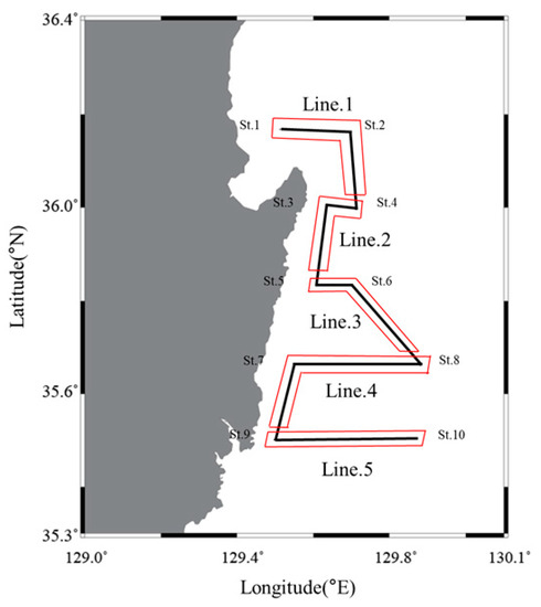
Figure 1.
Survey Area.
2.2. Acoustic Equipment System and Data Analysis Method
The acoustic system used for the survey was a split-beam scientific echosounder (EK60, Kongsberg Simrad, Norway), and acoustic data were collected for frequencies 38 and 120 kHz. The acoustic data were stored by continuously receiving position information from DGPS (SPR-1400, Samyoung, Seongnam, Korea). The acoustic data collected in situ were subsequently processed in the laboratory using acoustic data analysis software (Echoview V 8.0, Echoview Software Pty Ltd., Hobart, Australia). The flow diagram of data processing for the fish species identification is shown in Figure 2. As shown in the figure, after filtering the noise around the sea surface, sea bottom, and other places, the integration section is set to compose a matrix for each frequency, thus creating a new echogram. In this study, a cell size of 5 ping × 5 m (width × height) was used to examine the dB-difference. When the dB-difference between fish species becomes clear, the range of values is set, the data range bitmap is created, and the mask is created with an echo that matches the size of the cell at 38 kHz. We then extract echoes consistent with the 38 kHz echo, which is removed noise, by dividing them again into ping intervals. Through the above methods, fish species can be identified by separating the echoes of fish suitable for each characteristic.
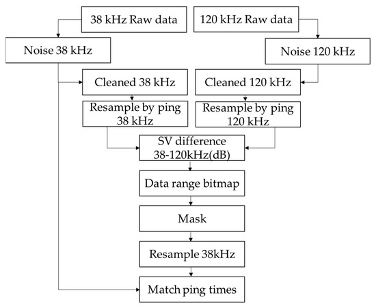
Figure 2.
Acoustic data post-processing analysis.
Using the above method and procedure, each species can be identified by separating the echoes of the respective fish species suitable for the characteristics [10].
2.3. Analysis of Sampled Fish Species
In order to identify fish species in the target waters for survey using the acoustic data, biological information of the fish species, such as composition and total length–body weight information of the fish species inhabiting the sea area, is required. Therefore, in this study, the total length–body weight information of fish was obtained using the bottom trawl survey, and the eDNA information of fish was acquired by collecting surface seawater within the survey area [11]. As a result of identifying fish species using eDNA information, the sampled species were 33.9% of Gadus macrocephalus, 28.3% of Clupea pallasii, 12.7% of Glyptocephalus stelleri, 4.6% of Engraulis japonicus, 4.2% of sea bass (Lates calcarifer), and 3.0% of jack mackerel Trachurus symmetricus. Therefore, the target fish species of this study were selected to be Gadus macrocephalus, Clupea pallasii, and Engraulis japonicus, which appeared as dominant fish species as a result of eDNA analysis. Todarodes pacificus, a major fish species in the East Sea, was additionally selected as the target species (Table 2).
Table 2.
List of fish species for analysis.
2.4. Acoustic Backscattering Strength
The range of total length of Gadus macrocephalus was 36.4–74.0 cm, and that of Engraulis japonicus was 9.5–15.4 cm. In addition, the range of total length of Todarodes pacificus was 16.0–27.0 cm, and that of Clupea pallasii was 12.0–27.0 cm. The total weight of the collected Gadus macrocephalus was 3459 g, and the total weight of Engraulis japonicus was 1910 g. Todarodes pacificus had a collection weight of 1235 g, and Clupea pallasii had a collection weight of 4617 g.
The frequency characteristics of each fish species for the dominant species were identified, and the results of a previous study were applied for the acoustic scattering characteristics for each frequency. Information on the acoustic scattering strength of the dominant species is presented as follows [12,13,14,15].
Gadus macrocephalus: TS38kHz = 24.8log (TL) − 73.1, TS120kHz = 17.9log (TL) − 61.5
Engraulis japonicus: TS38kHz = 16.7log (TL) − 62.8, TS120kHz = 15.9log (TL) − 64.7
Todarodes pacificus: TS38kHz = 12.9log (TL) − 63.7, TS120kHz = 20log (TL) − 73.5
Clupea pallasii: TS38kHz = 21.79log (TL) − 66.01, TS120kHz = 25.30log (TL) − 72.07
For the identification of fish species, the range of total length for each species and acoustic scattering strength were used to represent acoustic scattering strength for each frequency, and the frequency range was set using the dB-difference method. Therefore, the dB-difference range for Gadus macrocephalus was set to be −0.86 dB < ∆MVBS 38–120 kHz < 0.82 dB, and the dB-difference range for Engraulis japonicus was set to be 2.66 dB < ∆MVBS38–120 kHz < 2.84 dB. In addition, the dB-difference range for Todarodes pacificus was 0.36 dB < ∆MVBS38–120 kHz < 1.25 dB, and the range for Clupea pallasii was 0.88 dB < ∆MVBS 38–120 kHz < 2.28 dB. These ranges were set for fish species identification.
For the identification of fish species, it is necessary to first identify the frequency characteristics for the fish’s frequencies of 38 and 120 kHz and differences between them. In this case, the dB-difference represents the difference in the mean volume backscattering strength (MVBS) at multiple frequencies. To set ∆MVBS as positive values, target strength (TS) for each frequency of the target species for separation is compared, and the frequency with the smaller TS value is subtracted from the frequency with the large TS value. In general, the frequency of fish showed higher values at 38 kHz than at 120 kHz. Therefore, in a new echogram of 38 kHz and 120 kHz generated in the form of a matrix, ∆MVBS can be expressed by the following (Equation (1)).
The method for identifying each fish species is shown in the figure below by applying the sampled data and the acoustic scattering strength for each fish species (Figure 3, Figure 4, Figure 5 and Figure 6).
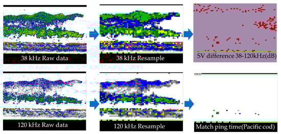
Figure 3.
Pacific cod identification example.
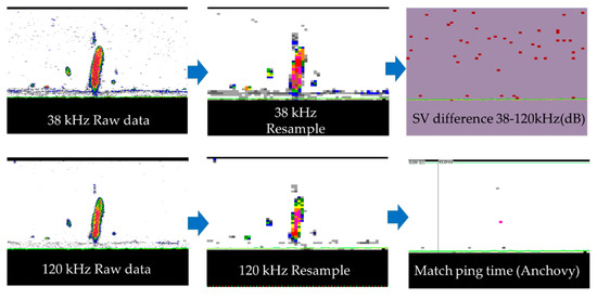
Figure 4.
Anchovy identification example.
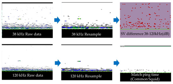
Figure 5.
Common squid identification example.
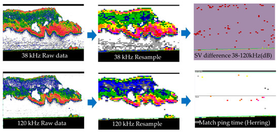
Figure 6.
Herring identification example.
3. Results
Vertical Distribution by Species
Using the dB-differences, the vertical distribution of Gadus macrocephalus is shown in the figure below, and the depth of the survey area was found to be in the range from 50 m to 250 m or more. The horizontal axis represents the time, the number at the top indicates the number of the survey line according to the movement of the survey line, the vertical axis represents the depth of water, and the thin solid line represents the water depth at 50 m intervals. The color scale on the right shows the intensity of sound waves received after they were reflected by the fish school. The higher the fish School, the darker brown that represents it.
At line 1, acoustic scattering layers in the range of −61 to −64 dB were distributed at the sea bottom with a depth of 50 m, and at line 2, acoustic scattering layers in the range of −52 to −64 dB were distributed at the sea bottom with a depth of 150 m. At line 3, with 100 m depth, acoustic scattering layers in the range of −52 to −64 dB were distributed, and at lines 4 and 5, acoustic scattering layers in the range of −56 to −67 dB were distributed. At lines 6 and 7, acoustic scatterers in the range of −61 to −70 dB were distributed at the sea bottom with a depth of 150 m. At lines 9 and 10 with 50 and 120 m depths, acoustic scattering layers in the ranges of −37 and −52 to −70 dB were distributed (Figure 7).
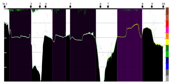
Figure 7.
Vertical distribution of pacific cod.
As a result of examining the distribution of Engraulis japonicus using the dB-difference, lines 1 and 2 did not show the echogram of Engraulis japonicus, and at lines 3 and 4, acoustic scattering layers in the ranges of −46 to −64 dB and −52 to −64 dB were distributed at 100 m depth. At line 5, acoustic scattering layers in the range of −64 to −70 dB were distributed at 100m depth, and at lines 6 and 7, acoustic scatterers in the range of −64 to −70 dB were distributed. At lines 9 and 10 with 50 and 100 m depths, acoustic scatterers in the ranges of −43 and −61 to −70 dB were distributed (Figure 8).
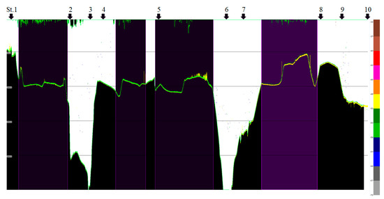
Figure 8.
Vertical distribution of pacific cod.
As a result of examining the distribution of Todarodes pacificus using the dB-difference, at line 1, acoustic scatterers in the range of −61 to −67 dB were distributed at a depth of 50 m, and at lines 2 and 4, acoustic scatterers in the range of −64 to −67 dB were distributed at a depth of 50–100 m. At line 5, acoustic scatterers in the range of −37 to −55 dB were distributed at 80 m depth, and at lines 6 and 7, acoustic scatterers in the range of −61 to −70 dB were distributed. At lines 9 and 10 with 50 m depth, acoustic scatterers in the range of −61 to −70 dB were distributed (Figure 9).
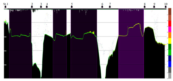
Figure 9.
Vertical distribution of common squid.
As a result of examining the distribution of Clupea pallasii using the dB-difference, at line 1, acoustic scattering layers at −46 and −61 dB were distributed at a depth of 50 m, and at lines 2 and 4, acoustic scatterers in the ranges of −37 to −46 dB and −52 to −64 dB were distributed at a depth of 50–100 m. At line 5 with 90 m depth, acoustic scattering layers in the range of −37 to −46 dB were distributed, and at lines 6 and 7, acoustic scattering layers in the range of −52 to −64 dB were distributed at a depth of 150 m. At line 8, acoustic scattering layers in the range of −37 to −46 dB were distributed at a depth of 50 m. At line 9, with 10 and 70 m depths, acoustic scattering layers in the ranges of −34 to −40 dB and −40 to −46 dB were distributed (Figure 10).
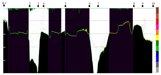
Figure 10.
Vertical distribution of herring.
As a result of examining the vertical distribution of each fish species, Gadus macrocephalus was mostly detected at the sea bottom, and Engraulis japonicus and Todarodes pacificus were mainly detected at a depth of 50 m. Clupea pallasii was mostly detected at a depth between 50 and 150 m.
4. Discussion
The results of previous studies on the distribution of fish species by water depth showed that Engraulis japonicus shoal was mainly distributed at a depth range of 12–50 m, and the volume scattering strength distribution of Engraulis japonicus shoal was around −50 dB. In addition, in another previous study, the volume scattering strength of the large Engraulis japonicus shoal with a high level of aggregation was in the range of −44.0 to −28.0 dB, and the large Engraulis japonicus shoal was distributed at a depth range of 10–75 m. Furthermore, the previous study on the distribution of Atlantic herring (Clupea harengus) by water depth showed the distribution of the species in the range of 10–125 m. A previous study on the distribution of Todarodes pacificus in the East Sea of South Korea showed the distribution of the species mainly at 60 m depth. Therefore, when comparing the results of this study with those of previous studies, it can be concluded that the distribution of species by depth was similar [14,15,16,17,18,19].
The spatiotemporal distribution of each fish species was represented by extracting the Nautical Area-Scattering Coefficient (NASC m2/nm2) and is illustrated in the figure below, and the size of NASC was represented by the height of the bar graph.
The results of the spatiotemporal distribution of Gadus macrocephalus showed a higher level of distribution in the south of the area, and a higher level of distribution was identified in coastal waters than in the open ocean. In addition, Gadus macrocephalus was distributed in the open ocean waters of Ulsan (Figure 11).
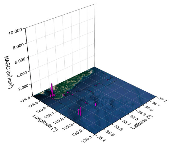
Figure 11.
Spatiotemporal distribution of pacific cod.
When comparing the results of this study with the results acquired by using the pop-up electronic tag for the movement route of Gadus macrocephalus, the location of recovering the Gadus macrocephalus pop-up tag in 2011 was 34.53° N, 128.49° E. Additionally, in the analysis result of the hydroacoustic survey, the identified location of distribution in the coastal waters was 35.5° N, 129.5° E. Furthermore, the location of recovering the pop-up tag in 2014 was 34.93° N, 128.84° E. In the analysis result of the hydroacoustic survey, the identified location of distribution in the open ocean was 35.5° N, 129.85° E. It was concluded that the movement route of Gadus macrocephalus shown in the result of previous studies and the location of the distribution of Gadus macrocephalus obtained using hydroacoustic survey were very similar. However, there is little research on Gadus macrocephalus movement, and, thus, it is thought that further studies are needed to obtain data on various routes of Gadus macrocephalus by year (Figure 12).
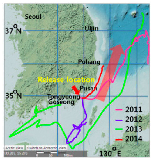
Figure 12.
The migration route of pacific cod [20].
The results of the spatiotemporal distribution of Engraulis japonicus showed high aggregation of the species in the coastal waters and open ocean of Ulsan in the survey area and low aggregation in the adjacent waters of Pohang. In a previous study that identified the distribution of Engraulis japonicus in the southern part of the East Sea, lower aggregation of the species was shown in coastal waters of Pohang, and high aggregation was observed in coastal waters and open ocean of Ulsan. Comparing the two sets of results, it is judged that the two results are considerably similar in many aspects [16]. However, the Engraulis japonicus shoal is a migratory species and shows aggregation at various depths, and, thus, further research is thought to be necessary (Figure 13 and Figure 14).
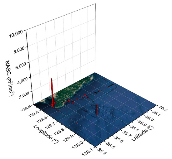
Figure 13.
Spatiotemporal distribution of anchovy.
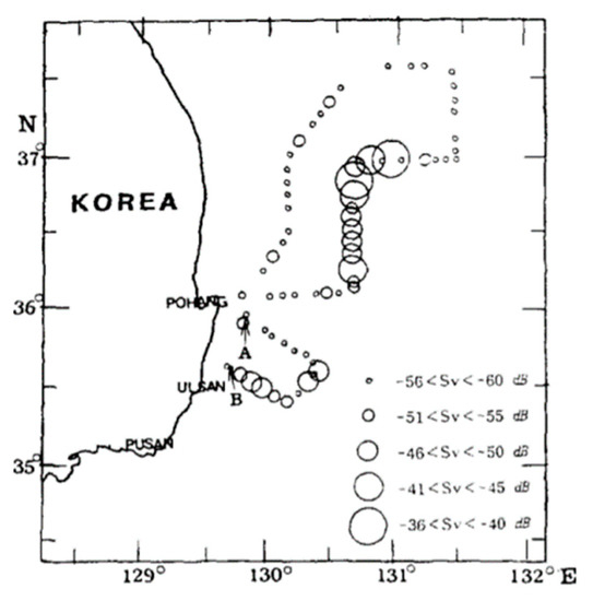
Figure 14.
Hydroacoustic investigations on the distribution characteristics of the anchovy at the south region of East Sea [17].
The spatiotemporal distribution of Todarodes pacificus showed a high aggregation in the coastal waters and open ocean in Ulsan and a relatively low aggregation in the coastal waters of Pohang (Figure 15).
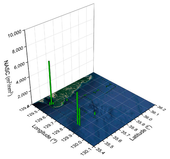
Figure 15.
Spatiotemporal distribution of common squid.
The spatiotemporal distribution of Clupea pallasii was relatively high in the coastal waters and open ocean of Ulsan and the northern waters of Ulsan, whereas the distribution was relatively low in the coastal waters of Pohang and adjacent sea (Figure 16).
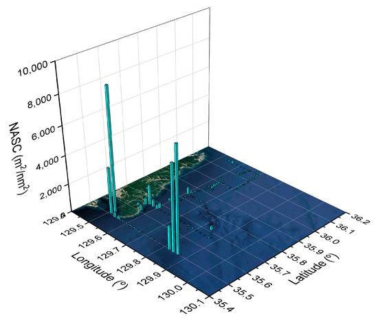
Figure 16.
Spatiotemporal distribution of herring.
This study used dB-difference to identify the species, space, and time distribution in the southern part of the East Sea waters of the Republic of Korea using various methods and distribution. Fish species were identified using frequencies of 38 and 120 kHz, but the distribution of fish species with similar target strengths and lengths can be mixed. However, since the fish species mainly distributed in the research waters of this study are the target fish species of the study, it is considered that the rate of other fish species is quite low.
Author Contributions
Conceptualization, D.-J.H., D.-S.K.; methodology, W.-S.O., K.-H.L.; software, W.-S.O., K.-H.L.; validation, Y.-W.L., D.-S.K.; formal analysis, W.-S.O., Y.-W.L.; investigation, Y.-W.L., D.-S.K.; resources, W.-S.O., K.-H.L.; data curation, D.-J.H., D.-S.K.; writing—original draft preparation, W.-S.O., K.-H.L.; writing—review and editing, W.-S.O., K.-H.L.; visualization, Y.-W.L., D.-S.K.; supervision, Y.-W.L., K.-H.L.; project administration, D.-J.H.; funding acquisition, D.-J.H. All authors have read and agreed to the published version of the manuscript.
Funding
This research was supported by the project entitled “Development of Advanced Science and Technology for Marine Environmental Impact Assessment” [grant number 20210427], funded by the Ministry of Oceans and Fisheries of Korea (MOF), and was partially supported by the Prime Cooperative Laboratory Program funded by Korea Maritime Institute, Korea.
Institutional Review Board Statement
Not applicable.
Informed Consent Statement
Not applicable.
Data Availability Statement
Not applicable.
Acknowledgments
This work was supported by the project entitled “Development of Advanced Science and Technology for Marine Environmental Impact Assessment” [grant number 20210427], funded by the Ministry of Oceans and Fisheries of Korea (MOF), and was partially supported by the Prime Cooperative Laboratory Program funded by Korea Maritime Institute. We are grateful to an editor and anonymous reviewers for their insightful comments that greatly helped to clarify and refine the paper.
Conflicts of Interest
The authors declare no conflict of interest.
References
- Lee, T.W. Seasonal variation in species composition of demersal fish in the coastal Water off Uljin and Hupo in the East Sea of Korea in 2002. Korean J. Ichthy. 2011, 23, 187–197. [Google Scholar] [CrossRef][Green Version]
- Kang, J.H.; Kim, Y.G.; Park, J.Y.; Kim, J.K.; Ryu, J.H.; Kang, C.B.; Park, J.H. Comparison of fish species composition collected by set net at Hupo in Gyeong-Sang-Buk-Do, and Jangho in Gang-Won-Do, Korea. Korean J. Fish. Aquat. Sci. 2014, 47, 424–430. [Google Scholar] [CrossRef][Green Version]
- Kang, P.J.; Kim, C.K.; Hwang, S.W. Species composition of fishes collected by pot nets in Coastal Waters around Gampo in the East Sea of Korea. Korean J. Ichthy. 2015, 27, 233–237. [Google Scholar]
- Lee, C.R.; Park, C.P.; Moon, C.H. Appearance of cold water and distribution of zooplankton off Ulsan-Gampo area, Eastern coastal area of Korea. J. Korean Soc. Ocean Eng. 2004, 9, 51–63. [Google Scholar]
- Won, J.H.; Lee, Y.W. Spatiotemporal variations of marine environmental parameters in the South-western region of the East Sea. J. Korean Soc. Ocean Eng. 2015, 20, 16–28. [Google Scholar] [CrossRef]
- Kang, M.H.; Furusawa, M.; Miyashita, K. Effective and accurate use of difference in mean volume backscattering strength to identify fish and plankton. ICES J. Mar. Sci. 2002, 59, 794–804. [Google Scholar] [CrossRef]
- Kang, M.H. Acoustic method for discriminating plankton from fish in Lake Dom Helvecio of Brazil using a time varied threshold. J. Korean Soc. Fish. Technol. 2012, 8, 495–503. [Google Scholar] [CrossRef]
- Miyashita, K.; Aoki, I.; Seno, K.; Taki, K.; Ogishima, T. Acoustic identification of isada krill, Euphausia pacifica Hansen, off the Sanriku coast, north-eastern Japan. Fish. Oceanogr. 1997, 6, 266–271. [Google Scholar] [CrossRef]
- McKelvey, D.R.; Wilson, C.D. Discriminant classification of fish and zooplankton backscattering at 38 and 120 kHz. Trans. Am. Fish. Soc. 2006, 135, 488–499. [Google Scholar] [CrossRef]
- Echoview Myriax. 2019. Help File 9.0 for Echoview. Myriax Software Pty Ltd. Hobart. Available online: http://support.echoview.com/WebHelp/Echoview.htm (accessed on 8 January 2015).
- Barnes, M.A.; Turner, C.R.; Jerde, C.L.; Renshaw, M.A.; Chadderton, W.L.; Lodge, D.M. Environmental conditions influence eDNA persistence in aquatic systems. Environ. Sci. Technol. 2014, 48, 1819–1827. [Google Scholar] [CrossRef] [PubMed]
- Rose, G.A.; Porter, D.R. Target-strength studies on Atlantic cod (Gadus morhua) in Newfoundland waters. ICES J. Mar. Sci. 1996, 53, 259–265. [Google Scholar] [CrossRef]
- Kang, D.H.; Mukai, T.; Hwang, D.J. Acoustic target strength of Japanese common squid, Todarodes pacificus, and important parameters influencing its TS: Swimming angle and material properties. In Proceedings of the Oceans ’04 MTS/IEEE Techno-Ocean ’04, Kobe, Japan, 9–12 November 2004; Volume 1, pp. 364–369. [Google Scholar]
- Kang, D.; Cho, S.; Lee, C.; Myoung, J.G.; Na, J. Ex situ target-strength measurements of Japanese anchovy (Engraulis japonicus) in the coastal Northwest Pacific. ICES J. Mar. Sci. 2009, 66, 1219–1224. [Google Scholar] [CrossRef]
- Kawabata, A. Target strength measurements of suspended live ommastrephid squid, Todarodes pacificus, and its application in density estimations. Fish. Sci. 2005, 71, 63–72. [Google Scholar] [CrossRef]
- Massé, J.; Koutsikopoulos, C.; Patty, W. The structure and spatial distribution of pelagic fish schools in multispecies clusters: An acoustic study. ICES J. Mar. Sci. 1996, 53, 155–160. [Google Scholar] [CrossRef]
- Kang, M.H.; Yoon, G.D.; Choi, Y.M.; Kim, J.K. Hydroacoustic investigations on the distribution characteristics of the anchovy at the south region of East Sea. Bull. Korean Soc. Fish. Technol. 1996, 32, 16–23. [Google Scholar]
- Misund, O.A. Sonar observations of schooling herring: School dimensions, swimming behaviour, and avoidance of vessel and purse seine. Rapports et Procès-Verbaux des Réunions 1990, 189, 135–146. [Google Scholar]
- Choi, S.J.; Arakawa, H. Relationship between the catch of squid, Todarodes pacificus Steenstrup, according to the jigging depth of hooks and underwater illumination in squid jigging boat. Korean J. Fish. Aquat. Sci. 2001, 34, 624–631. [Google Scholar]
- Lee, J.H.; Kim, J.N.; Lee, J.B.; Choi, J.H.; Moon, S.Y.; Park, J.; Kim, D.N. Movement of Pacific cod Gadus macrocephalus in the Korean Southeast Sea, ascertained through pop-up archival tags and conventional tags. J. Korean Soc. Fish. Ocean Technol. 2001, 51, 624–629. [Google Scholar] [CrossRef]


Publisher’s Note: MDPI stays neutral with regard to jurisdictional claims in published maps and institutional affiliations. |
© 2021 by the authors. Licensee MDPI, Basel, Switzerland. This article is an open access article distributed under the terms and conditions of the Creative Commons Attribution (CC BY) license (https://creativecommons.org/licenses/by/4.0/).