Omnidirectional Robotic Platform for Surveillance of Particle Accelerator Environments with Limited Space Areas

Abstract

Intelligent robotic systems are becoming essential for inspections and measurements in harsh environments. This article presents the design of an omnidirectional robotic platform for tunnel inspection with spatial limitations. This robot was born from the need to automate the surveillance process of the Super Proton Synchrotron (SPS) accelerator of the European Organization for Nuclear Research (CERN), where there is remaining radiation. The accelerator is located within a tunnel that is divided by small doors of 400 × 200 mm dimensions, through which the robot has to cross. The designed robot brings a robotic arm, and the needed devices to carry out the inspection. Thanks to this design, the robot application may vary by replacing certain devices and tools. In addition, this paper presents the kinematic and dynamic control models for the robotic platform.

1. Introduction

One of the most significant problems in underground tunnels is the survey of the proper performance of the security sensors available all along the whole corridor. Inspection of large tunnels can be laborious when performed by operators. However, robots may help with performing 4D tasks (dirty, dangerous, difficult, and dull), reducing risks for the personnel. Inspection in underground tunnels use to be complicated because of (a) the long time to access the facilities, (b) the long time to escape the facilities in case of evacuation, (c) the strong safety protocols, and (d) the lack of GPS signal to locate where you are. Usually used tunnels have other ways to communicate with the outside, such as 4G and a WiFi network.

To enhance the process of inspection in long tunnels, a robotic platform is presented in this paper. This mobile robot has been focused in the surveillance of the SPS where a large amount of restriction are present due to its actual state. However, the platform could be used in any other underground tunnel, where the only requirement is found in the floor material, which should guarantee that the omnidirectional wheels work properly.

The SPS is the second largest machine in CERN’s accelerator complex, with a circumference of approximately 7 km. Like the rest of tunnels of these characteristics, the corridor of the tunnel becomes completely monotonous, making navigation and SLAM an authentic challenge. Environmental sensors, which measure the radiation, temperature and oxygen concentration among others, are essential to guarantee material and personal safety. Due to the need of periodic check-ups of the sensors, inspections have to be carried out every month. Thus, in this paper we propose the design of an omnidirectional wheeled robot. The robot should be stored in a charging station, located in one of the entrances of the tunnel, where the batteries are charged. When required, it has to go around the ring and record data about the environmental variables. During its journey, the robot brings the needed sensors to record these variables and locate itself in the environment.

One of the most challenging features of the SPS is the fact that it has 19 partition doors which separate sections of the tunnel. These doors have an aperture of 400 × 200 mm, allowing the robot to cross them. Furthermore, the charging station is located in an area of difficult access. It means that the robot has to do several maneuvers to enter and go out of the station. In conclusion, the wheeled robot has the following requirements:

• The survey should take around 80 min. To achieve that, the robot should drive at a speed of 5.5 km/h, or 1.5 m/s, approximately.
• The robot should be able to deal with small spaces, such as doors of 200 × 400 mm.
• The motors should guarantee the nominal velocity of the robot of 5.5 km/h.
• The robot’s autonomy should be of 3 h at least, guaranteeing that the robot completes the surveillance even with the presence of unforeseen circumstances.
• The robot should be equipped with the required devices to perform the surveillance autonomously, or through tele-operation if the situation requires it. Autonomous inspection is understood as the fact that the robot travels through the tunnel without direct control by an operator. In such a way, that the robot is able to leave the charging station until the start of the journey, navigate from door to door, cross the door to go from one section to another, and go back to the charging station to charge the batteries. In this line, it is expected that the robot will need external sensors, such as cameras, a 3D LIDAR, and distance sensors to be placed in the middle of the tunnel.

The paper is organized as follows: In Section 2, an overview of wheeled robots is presented. In Section 3, we present the reasons which justify the selected locomotion arrangement. Later, we explain the selection of the locomotion actuators, the electronic and electrical design, the selection of the needed sensors to comply with the robot applications, and the mechanical design, where all the previous is included. Section 4 includes the kinematic and dynamic models of the robot for the locomotion arrangement selected, which will help us move the robot as desired. Section 6 includes the results of the design. Lastly, in Section 7, we present the conclusions of the developed work.

2. Related Work

Wheeled mobile robots are widely used in a large variety of applications, such as in industries, inspection, domestic tasks, rescue, planetary exploration, mining, hazardous waste clean-up, and medical assistance, among others. These robot may have different arrangements, such as differential, synchronous, tricycle, ackerman, or omnidirectional.

Differential drive mobile robots use two steering wheels with a free balancing wheel, called “castor”. These robots are controlled by two motors independently, are non-holonomic, have good manoeuvring capacities and work well in indoors environments [1]. However, the speed of these robot is very limited and the odometry estimation is very sensitive. To solve the last problem, backstepping methods for posture tracking [2], adaptive controllers to compensate errors and improve stability [3], and non-linear controllers [4] are used. Furthermore, a wheel synchronization is a critical point for the orientation control of differential mobile robots. Sun et al. propose in [5] a control approach for improving the orientation control, focusing in the coordination of the wheels instead on the robot configuration.

Synchronous drive mobile robots use chains or belts to orientate the wheels at the same time to move the robot in the same direction. This kind of locomotion arrangement needs a lot of space to include all the needed devices. Even with the easiness of its control and the good accuracy of its proprioceptive sensors, its use is not very widespread in robotics mainly because of design problems. They may have as many wheels as desired, but usually they have three or four. Zaman et al. present in [6] a model for translation of a synchoronous drive mobile robot of three wheels, whereas Wada presents in [7] the concept of a variation of this kind of arrangement, making use of four “synchro-caster” wheels.

Tricycle mobile robots have never attracted attention in the scientific community due to its structure, bad stability, and complexity in the path planning in narrow environments. Kamga et al. present in [8] a path tracking controller for this kind of robot, where problematic dynamic effects are neglected.

Ackerman vehicles, as the one presented in [9], are required when an aggressive steering is needed while maintaining a reasonable velocity when positioned in flat surfaces with obstacles. However, this locomotion arrangement increases the design components (and design complexity), as well as it reduces the manoeuvrability. This kind of locomotion arrangement is widely used in agriculture.

Lastly, omnidirectional robots are capable of moving in arbitrary directions without changing the direction of the wheels, thanks to the smart design of the mecanum wheels, ball wheels, or off-centered wheels among others. In order to increase stability and enhance manoeuvrability of omnidirectional robots with high heights and small bases, a reconfigurable footprint mechanism is developed in [10], which allows varying the ratio of wheel base to tread so that the vehicle could go through a narrow doorway, ensuring the stability. Similarly, the design of a four wheeled omnidirectional mobile robot with a variable wheel arrangement mechanism is presented in [11], where they take advantage of the redundant d.o.f. to drive the mechanism enabling the wheel arrangement to vary. Similarly, Byun et al. present in [12] an omnidirectional robotic platform with the capability of modifying the orientation of the wheels in order to save energy under some circumstances. These approaches would help a robot cross a door as described in Section 1; however, they only allow the platform to move at very slow velocities. Moreover, they do not have into account the viability of using the systems in machines with spatial constraints, since the systems require a mechanical connection between the four wheels, throughout a free joint.

Similarly to our requirements, in [13] an omnidirectional wheeled robot is developed with the objectives of manipulating objects and navigating in indoor environments. They mount two 3D LIDARs, one in front and one in the back, in order to have autonomous navigation in indoors environments. They focus the design on a robotic arm with high load capabilities, without focusing on spatial constraints. In addition, the disposal of the 3D LIDARs produces (a) the necessity of a very accurate calibration to join the generated point clouds, (b) the limitation of navigation only in indoors environments with a lot of features (unable to implement in tunnels), and (c) high costs due to the location of two sensors. Jia et al. present in [14] a kinematic model of a mecanum wheeled robot of four wheels. Later they design and develop the robot. The design approach does not take advantage of the free space between the wheels, raising the load within the body of the platform. Equally, Liu et al. present in [15] an omnidirectional robotic platform with for mecanum wheels and a manipulator. By mounting a manipulator in this kind of arrangement, the working space is expanded. Lastly, since this locomotion arrangement produces an unavoidable glide, ref. [16,17] study the movement performance of mecanum wheeled omnidirectional mobile robots, trying to solve the problem of determining the robot pose even though the robot slides.

About trading platforms, many large manufacturers sell omnidirectional robotic platforms, such as KUKA with the Kuka Mobile Platform 1500, Stanley with Flex Omni, or Nexus with Mecanum 4WD. However, all these platforms are much larger than ours required, in addition to not leaving free the possibility of including a robotic arm to carry out maintenance and handling tasks.

3. Omnidirectional Robotic Platform. Hardware Design

According to the requirements described in Section 1, we have decided to select an omnidirectional locomotion arrangement, with four mecanum wheels located in parallel. Mecanum wheels are composed by passive rollers that transform the force to other directions, giving the robot the capability to be omnidirectional. The selected wheels have a frame that covers the rubber rollers. They work properly on smooth and hard surfaces, such as the tunnel floor, excluding in the same way the necessity of damping devices due to the regularity of the surface.

With the chosen locomotion structure, where the wheels are located in a rectangle with straight forward orientation, we denote important advantages. First of all, (a) the design is more simple, since each wheel has only one associated motor set. (b) The robot is more compact, since the wheels are mounted in the covering box of the whole robot, giving important advantages when crossing the doors or when entering in the charger station. (c) The risk when a motor fails is lower, giving more robustness against foreseen failures in one of the wheels. This kind of structure makes the system redundant, this is, there are more modifiable d.o.f., four in this case, than motion d.o.f, three in this case ($x,y,\theta$). That means that in case a motor fails, the system would be able to finish its task through the implementation of fault tolerance techniques and control architecture approaches. However, this locomotion arrangement presents some disadvantages that should be taken into account: (a) the rollers of the wheels usually slide, spoiling slightly the odometry estimation of the wheels, and (b) the energetic efficiency is low. These problems are not critical, since (a) a SLAM system may correct the wrong odometry, (b) the wheeled robots allow enough space for the batteries to cover the task energetic requirements, and (c) the required speed is low for safety reasons, since the robot is expected to be autonomous in an environment where crashes are not allowed.

Intending to comply with the requirements (surveillance time, robot speed, spatial constraints, autonomy time and tele-operation availability), we present along this section the selection of the locomotion actuators, the electronic and electrical design, the selection of the needed sensors to comply the robot applications, and the mechanical design, where all the previous is included.

3.1. Locomotion Calculation

We present the guidelines to determine the proper motor, gearhead, and encoder. It is important to highlight that the wheels have a known size. They have been selected during the mechanical design process, and they have a crucial role in the selection of the motor set since the most critical part is found in the acceleration torques, which have a strong dependency on the moments of inertia. Firstly, we calculate the nominal force, torque, and power that each motor set has to provide, this is, when the robot is driving at the desired nominal speed. Secondly, we find out the maximum force, torque, and power, which are highly related to the inertial moments, this is, when the robot is under acceleration. With all these calculations, we choose the required devices, which eventually are tested in simulation.

3.1.1. Nominal Torque and Power

Equation (1) relates the desired linear velocity of the robot, $V_{nom}$, with the angular velocity of the wheels in r.p.m., $n_{nom}$. Here, a factor $\eta$ is applied to ensure good performance even with the inevitable presence of friction.

$$n_{nom}=\frac{60}{\pi }·\frac{V_{nom}}{d·\eta }$$

(1)

On the other hand, (2) calculates the nominal torque, $M_{nom}$, to move the entire robot at nominal velocity. This torque depends proportionally on the force necessary to apply, $F_{nom}$, which is determined in (3), and inversely on the bearing factor, $\delta$.

$$M_{nom}=\frac{d}{2}·\frac{F_{nom}}{\delta }$$

(2)

The nominal force is the needed force to keep the robot at the nominal velocity. Typically, three main friction forces appear during the displacement of a vehicle: (a) rolling resistance, (b) aerodynamic resistance, and (c) slope resistance. Both aerodynamic and slope resistances may be neglected in our case. Aerodynamic resistance does not contribute because of the following reasons: (a) the air in the tunnel is static, without the presence of air currents, (b) the robot moves at low velocity, and (c) the air is clean and dry. Slope resistance does not contribute because the tunnel is mainly flat. Thus, the rolling force is calculated in (3) through (a) the rolling resistance coefficient, or the coefficient of rolling friction (CRF), $C_{rr}$, and (b) the normal force, $F_N$, this is, the perpendicular force to the surface on which the wheel is rolling. The coefficient of rolling friction is given in (4) [18] by the sinking depth, z, which depends on the elastic features of the material of the rollers, and the wheel diameter, d. On the other hand, $F_N$ depends on the robot weight, $m_R$.

$$F_{nom}=C_{rr}·F_N=C_{rr}·m_R·g$$

(3)

$$C_{rr}=\frac{z}{d}$$

(4)

The calculated nominal torque has to be split in the number of traction wheels, N, in the robot, as expressed in (5), resulting in the needed nominal torque in each motor set, $M_{nom/m}$.

$$M_{nom/m}=\frac{M_{nom}}{N}$$

(5)

So far, the torque when the nominal velocity is reached has been calculated. However, in order to calculate the acceleration, average and maximum torques, a velocity profile has to be created, as shown in Figure 1, where the time to reach the nominal velocity, $t_{acc}$, and the time of nominal velocity, $t_{nom}$, are indicated. For simplicity, we have assumed constant acceleration, a, and equal acceleration and deceleration time. Thus, acceleration is calculated in (6).

$$a=\frac{V_{nom}}{t_{acc}}$$

(6)

The last variable to figure out is the power that the motor set has to provide while the robot is driving at nominal velocity. Thus, in (7) we calculate the necessary nominal power of the motor set, $P_{nom/m}$, where a confidence factor, $\kappa$, and a power factor, $PF$, have been set to slightly oversize the set. Anyway, the chosen devices have to provide more power than calculated during the nominal stage.

$$P_{nom/m}=PF·\frac{m_R·V_{nom}·(a+g·sin\theta )}{2·\pi ·\kappa ·N}$$

(7)

3.1.2. Maximum Torque and Power

One of the most important parts in the selection of the locomotion actuators is found in the inertial forces, this is, the force that the locomotion system has to apply during the acceleration and deceleration. With a preliminary motor selection, it is possible to know its moment of inertia. Since the wheels and shaft ones are well known, the one of the full system, this is motor/shaft/wheel, may be calculated. Both wheel and shaft ones, $J_w$ and $J_s$, respectively, are calculated through (9), where the inertial mass, $m_i$, is calculated in (8). Here, we define (a) $\rho$ as the component density, (b) $r_a$ as its external radius, (c) $r_i$ as its internal (if applicable), and (d) h the width.

Thus, the robot acceleration torque, $M_{acc}$, is calculated in (10), where the moment of inertia of the motor, $J_m$, is one of the motors that satisfies the previous specifications, and where d is the diameter of the wheels. Although the moment of inertia of the motor may change with the final decision, it is practically negligible concerning that of the set of wheel, shaft, motor, and robot weight (each one is indicated in (10).

$$m_i=\rho ·\pi ·({r_a}^2-{r_i}^2)·h$$

(8)

$$J_w=\frac{1}{2}·m_i·({r_a}^2+{r_i}^2)$$

(9)

$$M_{acc}=(N·(\underset{wheel}{\underbrace{J_w}}+\underset{motor}{\underbrace{J_m}}+\underset{shaft}{\underbrace{J_s}})+\underset{robot}{\underbrace{\frac{m_R}{\eta }·\frac{d^2}{4}}})·a·PF$$

(10)

Then, taking into account the torque during the nominal moment (2) and during the acceleration (10), it is possible to calculate the maximum and the root mean square, RMS, torque in each motor, $M_{max/m}$ and $M_{rms/m}$, respectively, according to (11), (13) and (14), respectively. For a wheeled robot, the decelerate torque, $M_{dec}$, is determined by the difference between the nominal and acceleration torques, as indicated in (12). For a robotic platform that is continuously working, the resting torque, denoted as $M_{rest}$ is null, since the robot is expected to perform the survey without stops.

$$M_{max/m}=\frac{M_{max}}{N}=\frac{M_{nom}+M_{acc}}{N}$$

(11)

$$M_{dec}=M_{nom}-M_{acc}$$

(12)

$$\begin{array}{c}\hfill M_{rms}=\{\frac{1}{t_{total}}·(t_{acc}·M_{max}^2+t_{nom}·M_{nom}^2+\\ \hfill t_{dec}·M_{dec}^2+t_{rest}·M_{rest}^2){\}}^{1/2}\end{array}$$

(13)

$$M_{rms/m}=\frac{M_{rms}}{N}$$

(14)

After all, the maximum and RMS power may be calculated according to (15) and (16), respectively.

$$P_{max/m}=M_{max/m}·n_{nom}·\frac{\pi }{30}$$

(15)

$$P_{rms/m}=M_{rms/m}·n_{rms}·\frac{\pi }{30}$$

(16)

3.1.3. Motor and Gearhead Selection

Thanks to the equations described before, we should select a gearhead with a continuous torque of at least $M_{rms/m}$, and an intermittent torque at gear output of at least $M_{max/m}$. In our case, we have chosen the model GP 26A of Maxon, which has a reduction of $K_g$ of 1:27 and a maximum efficiency $\eta$ of 80%. It is required to select the immediately inferior reduction that fulfills the requirements.

After that, we should chose a motor that provide (a) an angular velocity of at least $n_{nom}·K_g$ (r.p.m.), (b) a continuous torque of at least $M_{rms/m\prime }$, calculated in (17), (c) a maximum torque of at least $M_{max/m\prime }$, calculated in (18), and (d) a continuous operation power of at least $P_{rms/m}$.

$$M_{rms/m\prime }=\frac{M_{rms/m}}{K_g·\eta }$$

(17)

$$M_{max/m\prime }=\frac{M_{max/m}}{K_g·\eta }$$

(18)

Then, it is needed to check that the speed constant of the motor is at least $C_v$, calculated in (19). Here, $V_0$ denotes the no-load speed calculated in (20), whereas $\upsilon$ denotes the voltage of the motor. Regarding the no-load speed equation, $\tau$ denotes the speed/torque gradient of the motor.

$$C_v=\frac{V_0}{\upsilon }$$

(19)

$$V_0=V_{nom}+\tau ·M_{max/m\prime }$$

(20)

In the end, we have chosen the motor model RE 25, Graphite Brushes, 20 W of 24 V, which fulfills the previous specifications. Additionally, we select the encoder model Encoder MR Type ML, which allows 500 counts per turn, high enough to guarantee real-time behavior for a wheeled robot.

For mechanical reasons, it is needed a motion transmission between the motor system and the wheels. To solve this problem, a couple of pulleys, connected by a belt, are used. Taking advance of this restriction, a velocity reduction is applied to get the nominal robot velocity. The relationship of the pulleys in our case is 1:1.1.

3.1.4. Electronic and Electrical Design of the Motor Set

Since the motor, the gearhead, the encoder, and the controller (EPOS4 Compact 50/5) have been selected from Maxon Motor seller, the cables have been chosen as well. In order to communicate the controller with the computer, we have used CAN bus, as shown in the electronic and electrical scheme shown in Figure 2. The electronic and electrical scheme shows each cable with the corresponding identifier of the seller.

3.1.5. Motor Validation

In order to guarantee the proper performance of the selected motor and gearhead, we have simulated the motor set behavior under the expected circumstances during the driving. Thus, the simulation shows the performance of the motor set when the robot follows the velocity profile described before.

In this way, simulating the behavior of the motor, we have developed the block diagram illustrated in Figure 3, where we include a PID controller that directly control the motor model (defined by its features such as the terminal resistance, terminal inductance, torque constant, inertial moment and viscous constant).

$M_{in}$ denotes the load reaction torque, this is the torque produced by the robot weight, friction, slope of the terrain, etc. This torque is related to the force specified in (3). Thus, the simulation process follows the following guidelines:

• Guided by the high level controller, the desired velocity, $V_d$, is inserted.
• The PID controller takes the difference between the desired velocity and the current robot velocity, $V_R$, to generate the control signal, ${\upsilon }_c$, which is inserted in the model of the motor.
• The angular velocity of the motor is transformed to the robot velocity (linear) through the reduction generated by the gearhead and the pulleys, $K_n$. On the way, a friction constant is applied, $\eta$, as well as a transformation between angular to linear.

The obtained results for the required velocity show us that the motor does not reach its limits, concluding that the selected devices are proper for the first and third requirements described in Section 1.

3.2. Device Selection

In the final version, the robot will be equipped with the following sensors:

• Two 2D LIDARs for object detection. They will be used to prevent the robot from crashing with obstacles, with the walls, and with the accelerator. The model UST-20LX, by Hokuyo, is used.
• Cameras for teleoperation and optionally for visual odometry. The model UI-3080CP Rev. 2, by IDS, is used.
• A point cloud generator sensor for the self-localization. It can be a 3D LIDAR or an RGBd camera (only for small environments). The model HDL-32E of Velodyne has been used for localization and environment reconstruction tests with good results. However, it is recommendable to use another sensor like Puck Lite or Ultra Puck from the same manufacturer, since the size of this sensor is too big for our spatial constraints, the vertical field of view is focused down (problematic for low and small robots like ours) and it has moving parts (recommendable to avoid them). In this paper, we include the 3D LIDAR Puck Lite, by Velodyne.
• An inertial measurement unit, IMU, for the localization system. The model VMU931 is used.
• A radiation sensor.
• An ultrasonic sensor, SONAR, to determine the distance between the radiation sensor and the radiation source. The model MB7040 I2CXL-MaxSonar-WR Ultra compact Housing, by MaxBotix is used.
• A WiFi antenna for communication.
• A robotic arm to bring the radiation sensor in the particular application of the radiation survey, and to bring a specific tool in other cases. The Jaco by Kinova is used.

Furthermore, the onboard computer is the NUC i5-8259U, 8 GB, DDR4-SDRAM, 256 GB SSD Mini, by Intel, which is the computer that supports all the logic behavior. The devices are connected to the NUC as shown in Figure 4. We have decided to connect the cameras through Ethernet, whereas the robotic arm through USB drivers. However, both the cameras and the arm may use Ethernet or USB. With these devices, the system fulfills the needs to comply with the last requirement of Section 1.

3.3. Mechanical Design

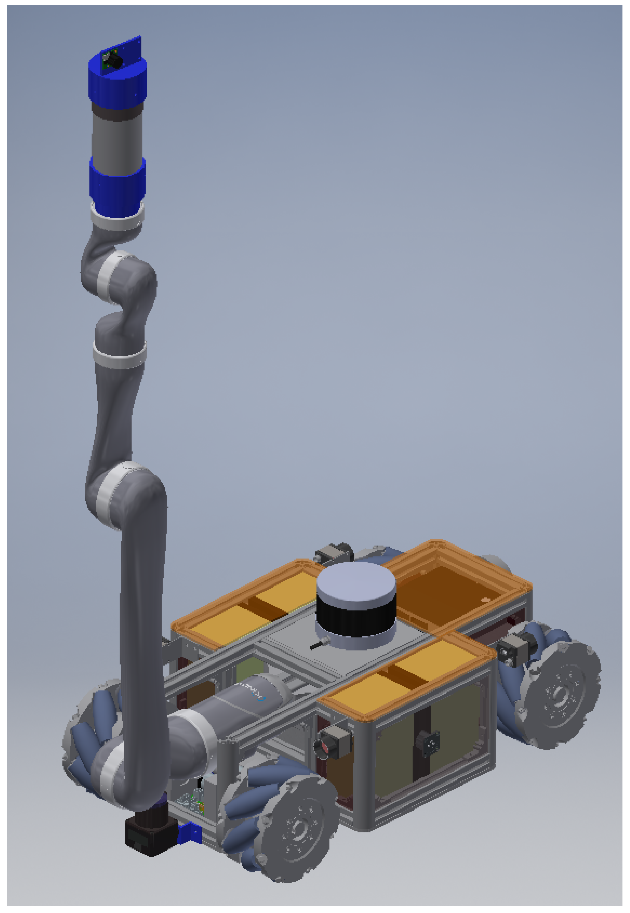
We present a mechanical design based on the use of aluminum profiles for the main structure, giving consistency and strength to the robot body. Furthermore, the bottom plates are also of aluminum material, since this material is proper for radioactive environments. The design (Figure 5) has the following characteristics:

• Four lead–acid batteries, two located at each side. Each provides $7A·$ h. In total they provide energy so that all the robot devices are working at their maximum power for 3 h and a quarter, enough to guarantee the forth requirement of Section 1.
• A magnetic connector for charging the batteries is localized on one side.
• Four possible localization for cameras behind the wheels, place where the field of view is good enough.
• Two 2D LIDAR for obstacle and wall detection (one in front and one in the back). Both of them are linked to the structure with a piece that has to be manufactured in aluminum material.
• A 3D LIDAR for the SLAM algorithm.
• A support for the radiation sensor in the end-effector of the robotic arm.
• A support in the radiation sensor to place the SONAR.

The main dimensions are 707 × 350 × 184 mm, a proper size to cross the doors, complying with the second requirement of Section 1. The estimation of the weight is around 45 kg, taking into account all the components. The reach of the sensor is around 1100 mm at its main point.

The robot adopts the position shown in Figure 6 when it is crossing the door, where it is appreciated that space while doing so is enough. In this configuration, the robotic arm is set horizontally and the 3D LIDAR is folded against the other face of the plate that supports the robotic arm.

The robot has been designed with an eye on the main application, this is, the surveillance of the SPS accelerator. However, with the cameras and with the robotic arm, the application range increases abruptly, having the possibility of using the robot in teleoperations (drilling, leak repair, component replacement, cable welding, etc.), visual surveillance of other environments, variable checking (temperature, oxygen concentration, etc.), and many more, with the single replacement of the end-effector tool.

4. Kinematic and Dynamic Models of the Robotic Platform

In this section, the kinematic and dynamic models of the platform are presented from a theoretical point of view, to include them into the CERNTAURO framework [20], which contains all the robotic software of CERN.

4.1. Kinematic Model

Firstly, to describe the robot posture in the ground plane, the reference systems shown in Figure 7 have been created, where we find reference systems of: (a) the world, ${\sum }_W$, (b) the robot, ${\sum }_R$, (c) the wheel i with the same orientation that the robot one, ${\sum }_{Ri}$, and (d) the wheel i with the orientation of the mecanum wheel rollers, ${\sum }_{ri}$.

In that picture, we describe: (a) the distance between ${\sum }_R$ and ${\sum }_{Ri}$, $L_i$, (b) the angle between the axis $R_x$ and the contact point of the wheel i rollers with the floor, ${\alpha }_i$, (c) the angle between the axis $r_{ix}$ and the axis $R_{iy}$, ${\beta }_i$, and (d) the angle between the axis $R_{iy}$ and the axis $r_{iy}$, ${\gamma }_i$. All of them are well known: (a) $L_i$, (b) ${\alpha }_i$ and (c) ${\beta }_i$ are determined by the dimensions of the robot design, and (d) ${\gamma }_i$ is determined by the wheel design (usually 45°). Moreover, we describe (e) ${\varphi }_i$ as a sum of ${\alpha }_i$, ${\beta }_i$ and ${\gamma }_i$, and (f) ${\delta }_i$ as a sum of ${\beta }_i$ and ${\gamma }_i$.

Like the vast majority of wheeled robots, the position of the robot is described by 3 d.o.f., this is, position and orientation x, y and $\theta$. Thus, the vector $\xi$ which defines the posture of the robot is presented in (21). Furthermore, we define (a) $\dot{\xi }$ as the velocity vector of the robot in ${\sum }_W$, and (b) $\eta$ as the velocity vector of the robot in ${\sum }_R$, calculated from $\dot{\xi }$ in (22), where $R_w^R\left(\theta \right)$ is the rotation matrix between ${\sum }_R$ and ${\sum }_W$.

$$\xi =\left[\begin{array}{c}x\\ y\\ \theta \end{array}\right]\in {\Re }^3$$

(21)

$$\eta =R_w^R\left(\theta \right)·\dot{\xi }=\left[\begin{array}{ccc}{c}_{\theta }& s_{\theta }& 0\\ -s_{\theta }& c_{\theta }& 0\\ 0& 0& 1\end{array}\right]·\left[\begin{array}{c}\dot{x}\\ \dot{y}\\ \dot{\theta }\end{array}\right]$$

(22)

The required velocity in each wheel i, ${\dot{O}}_{Ri}$, to move the robot at a given velocity $\eta$ is described in (23). In addition, in $\eta$ the velocities are referred to ${\sum }_R$, so in (24) we displace them to ${\sum }_{ri}$ through the rotation matrix $R_R^{R_i}\left({\varphi }_i\right)$, which does so.

$${\left[\begin{array}{c}{\dot{O}}_{R_{i1}}\\ {\dot{O}}_{R_{i2}}\\ 0\end{array}\right]}^R=\left[\begin{array}{c}{\dot{x}}^R-L_i·s_{{\alpha }_i·}\dot{\theta }\\ {\dot{y}}^R-L_i·c_{{\alpha }_i·}\dot{\theta }\\ 0\end{array}\right]$$

(23)

$$\begin{array}{c}\hfill {\left[\begin{array}{c}{\dot{O}}_{R_{i1}}\\ {\dot{O}}_{R_{i2}}\\ 0\end{array}\right]}^{R_i}=R_R^{R_i}\left({\varphi }_i\right)·{\left[\begin{array}{c}{\dot{O}}_{R_{i1}}\\ {\dot{O}}_{R_{i2}}\\ 0\end{array}\right]}^R=\\ \hfill \left[\begin{array}{ccc}{s}_{{\varphi }_i}& -c_{{\varphi }_i}& 0\\ c_{{\varphi }_i}& s_{{\varphi }_i}& 0\\ 0& 0& 1\end{array}\right]·{\left[\begin{array}{c}{\dot{O}}_{R_{i1}}\\ {\dot{O}}_{R_{i2}}\\ 0\end{array}\right]}^R\end{array}$$

(24)

According to [21], we define: (a) the wheel speed, ${\dot{\phi }}_{R_i}$, (b) the wheel radius, $r_{R_i}$, (c) the roller speed, ${\dot{\phi }}_{r_i}$, and (d) the roller radius $r_{r_i}$. In our case, the robot values are shown in

Table 1. Kinematic parameters of our robot. Figure 8 shows each variable in the robot frame.

Wheel i	${\mathit{L}}_{\mathit{i}}$	${\mathit{\alpha }}_{\mathit{i}}$	${\mathit{\beta }}_{\mathit{i}}$	${\mathit{\gamma }}_{\mathit{i}}$	${\mathit{r}}_{{\mathit{R}}_{\mathit{i}}}$
1	L	$360-\alpha$	$\frac{\pi }{2}-{\alpha }_1$	$\frac{\pi }{4}$	r
2	L	$\alpha$	$\frac{\pi }{2}-{\alpha }_2$	$-\frac{\pi }{4}$	r
3	L	$180-\alpha$	$\frac{\pi }{2}-{\alpha }_3$	$\frac{\pi }{4}$	r
4	L	$180+\alpha$	$\frac{\pi }{2}-{\alpha }_4$	$-\frac{\pi }{4}$	r
L			274.06 mm
$\alpha$			29.5°
r			76.2 mm

.

For omnidirectional robots with mecanum wheels, the delivered speed by the wheel is $r_{R_i}·{\phi }_{R_i}$ in the $R_{ix}$ direction, whereas the roller lineal velocity is $r_{r_i}·{\phi }_{r_i}$ in the $r_{ix}$ direction. Thus, making use of (24), we transform the delivered speed by the wheel to ${\sum }_{r_i}$ in (25).

$$\begin{array}{c}\hfill \left[\begin{array}{c}{r}_{R_i}·{\dot{\phi }}_{R_i}·c_{{\gamma }_i}\\ r_{r_i}·{\dot{\phi }}_{r_i}+r_{R_i}·{\dot{\phi }}_{R_i}·s_{{\gamma }_i}\\ 0\end{array}\right]=\\ \hfill \left[\begin{array}{ccc}{s}_{{\varphi }_i}& -c_{{\varphi }_i}& L_i·c_{{\delta }_i}\\ c_{{\varphi }_i}& s_{{\varphi }_i}& L_i·c_{{\delta }_i}\\ 0& 0& 0\end{array}\right]·\eta \end{array}$$

(25)

For each wheel, a motion constraint, shown in (26), is obtained from the first row of the equation system of (25) [21].

$$\left[\begin{array}{ccc}-s_{{\varphi }_i}& c_{{\varphi }_i}& L_i·c_{{\delta }_i}\end{array}\right]·R_w^R\left(\theta \right)·\dot{\xi }+r_{R_i}·{\dot{\phi }}_{R_i}·c_{{\gamma }_i}=0$$

(26)

Thus, the motion constraints equation of the entire robot is shown in (27), where (a) $J_1$ is composed by the motion constraint rows of each wheel, as described in (26), and where (b) $J_2$ is defined by the wheel design. The results are the Equations (28) and (29), respectively.

$$J_1·R_w^R\left(\theta \right)·\dot{\xi }+J_2·{\dot{\phi }}_i=0$$

(27)

$$J_1=\left[\begin{array}{ccc}-s_{{\varphi }_1}& c_{{\varphi }_1}& L_1·c_{{\delta }_1}\\ -s_{{\varphi }_2}& c_{{\varphi }_2}& L_2·c_{{\delta }_2}\\ -s_{{\varphi }_3}& c_{{\varphi }_3}& L_3·c_{{\delta }_3}\\ -s_{{\varphi }_4}& c_{{\varphi }_4}& L_4·c_{{\delta }_4}\end{array}\right]$$

(28)

$$J_2=\left[\begin{array}{cccc}{r}_{R_1·}{c}_{{\gamma }_1}& 0& 0& 0\\ 0& r_{R_2·}{c}_{{\gamma }_2}& 0& 0\\ 0& 0& r_{R_3·}{c}_{{\gamma }_3}& 0\\ 0& 0& 0& r_{R_4·}{c}_{{\gamma }_4}\end{array}\right]$$

(29)

The kinematic configuration model for that robot is given by (30) [21], where $S\left(q\right)$ is decomposed in the high and low part, relating to the kinematic posture model and the wheels velocities, respectively.

$$\dot{q}=\left[\begin{array}{c}\dot{\xi }\\ \dot{{\phi }_1}\\ \dot{{\phi }_2}\\ \dot{{\phi }_3}\\ \dot{{\phi }_4}\end{array}\right]=\left[\begin{array}{c}\dot{x}\\ \dot{y}\\ \dot{\theta }\\ \dot{{\phi }_1}\\ \dot{{\phi }_2}\\ \dot{{\phi }_3}\\ \dot{{\phi }_4}\end{array}\right]=S\left(q\right)·\eta =\left[\begin{array}{c}{R}_w^R\left(\theta \right)\\ E\end{array}\right]·\left[\begin{array}{c}\dot{x^R}\\ \dot{y^R}\\ {\dot{\theta }}^R\end{array}\right]$$

(30)

The high part of the previous equation is determined by the kinematic posture model for an omnidirectional robot, which is given by (31). The low part of the equation is given by the isolation of $\dot{{\phi }_i}$ from (27), in such a way that for all the wheels we obtained (32), which is related to E from (30).

$$\dot{\xi }=R_R^w\left(\theta \right)·\eta$$

(31)

$$\dot{{\phi }_i}=-J_2^{-1}·J_1·R_w^R\left(\theta \right)·\dot{\xi }=-J_2^{-1}·J_1·\eta$$

(32)

Then, substituting the values of Table 1, we obtain our kinematic model, which is presented in (33).

$$\dot{q}=\left[\begin{array}{c}\dot{x}\\ \dot{y}\\ \dot{\theta }\\ \dot{{\phi }_1}\\ \dot{{\phi }_2}\\ \dot{{\phi }_3}\\ \dot{{\phi }_4}\end{array}\right]=\left[\begin{array}{ccc}{c}_{\theta }& -s_{\theta }& 0\\ s_{\theta }& c_{\theta }& 0\\ 0& 0& 1\\ \frac{1}{r}& \frac{1}{r}& \frac{(l_1+l_2)}{r}\\ \frac{1}{r}& -\frac{1}{r}& -\frac{(l_1+l_2)}{r}\\ \frac{1}{r}& \frac{1}{r}& -\frac{(l_1+l_2)}{r}\\ \frac{1}{r}& -\frac{1}{r}& \frac{(l_1+l_2)}{r}\end{array}\right]·\left[\begin{array}{c}\dot{x^R}\\ \dot{y^R}\\ {\dot{\theta }}^R\end{array}\right]$$

(33)

4.2. Dynamic Model

The dynamic model for a wheeled omnidirectional robot can be calculated through (34), where (a) the sum of kinetic energies of the robot, T, is calculated in (35), and where (b) the applied torque in the wheel i, $\phi$, is figured out in (36) [21].

$$R_w^R\left(\theta \right){\left[T\right]}_{\xi }+E^T{\left[T\right]}_{\phi }=E^T{\tau }_{\phi }$$

(34)

$${\left[T\right]}_{\psi }=\frac{d}{dt}\left(\frac{\partial T}{\partial \psi }\right)-\frac{\partial T}{\partial \psi }$$

(35)

$${\tau }_{\phi }={\left[\begin{array}{cccc}{\tau }_{\phi 1}& {\tau }_{\phi 2}& {\tau }_{\phi 3}& {\tau }_{\phi 4}\end{array}\right]}^T$$

(36)

We denote (a) $m_R$ as the robot total mass, (b) $I_{Rz}$ as the robot total moment of inertial, and (c) $I_{\phi y}$ a the wheels moment of inertial. For an omnidirectional robot, T can be expressed as shown in (37), where M, $I_{\phi }$ and $\dot{\phi }$ have the values shown in (38)–(40).

$$T=\dot{{\xi }^T}{\left(R_w^R\left(\theta \right)\right)}^T·M·R_w^R\left(\theta \right)·\dot{\xi }+\dot{{\phi }^T·I_{\phi }·\dot{\phi }}$$

(37)

$$M=\frac{1}{2}diag\left\{m_R,m_R,I_{Rz}\right\}$$

(38)

$$I_{\phi }=\frac{1}{2}diag\left\{I_{\phi y},I_{\phi y},I_{\phi y},I_{\phi y}\right\}$$

(39)

$$\dot{\phi }={\left[\begin{array}{cccc}\dot{{\phi }_1}& \dot{{\phi }_2}& \dot{{\phi }_3}& \dot{{\phi }_4}\end{array}\right]}^T$$

(40)

Developing (37), (41) is obtained.

$$\begin{array}{c}\hfill T=\frac{m_R}{2}\left({\dot{x}}^2+{\dot{y}}^2\right)+\frac{I_{Rz}}{2}{\dot{\theta }}^2+\\ \hfill \frac{I_{\phi y}}{2}\left({\dot{\phi }}_1^2+{\dot{\phi }}_2^2+{\dot{\phi }}_3^2+{\dot{\phi }}_4^2\right)\end{array}$$

(41)

${\left[T\right]}_{\xi }$ and ${\left[T\right]}_{\phi }$ terms are given using (35), whose results are reflected in (42) and (44).

$${\left[T\right]}_{\xi }=M_R·\ddot{\xi }$$

(42)

$$M_R=diag\left\{m_R,m_R,I_{Rz}\right\},\ddot{\xi }=\left[\begin{array}{c}\ddot{x}\\ \ddot{y}\\ \ddot{\theta }\end{array}\right]$$

(43)

$${\left[T\right]}_{\phi }=M_{\phi }·\ddot{\phi }$$

(44)

$$M_{\phi }=diag\left\{I_{\phi y}\right\},\ddot{\phi }\left[\begin{array}{c}{\ddot{\phi }}_1\\ {\ddot{\phi }}_2\\ {\ddot{\phi }}_3\\ {\ddot{\phi }}_4\end{array}\right]$$

(45)

Upgrading (34) with the previous calculations, (46) is obtained. In order to transform the accelerations from the world frame to the robot frame, (47) and (48) are presented. The second one uses and derives the high part of (33).

$$R_w^R\left(\theta \right)·M_R·\ddot{\xi }+E^T·M_{\phi }·\ddot{\phi }=E^T{\tau }_{\phi }$$

(46)

$$\ddot{\xi }=R_R^w\left(\theta \right)·\dot{\eta }+{\dot{R}}_R^w\left(\theta \right)·\eta$$

(47)

$$\ddot{\phi }=E·\dot{\eta }$$

(48)

The result is shown in (49), with (50) and (51), where the dynamic model of the omnidirectional robot is presented as the final model related to the operational space in (49)–(51).

$$\overline{M}·\dot{\eta }+\overline{C}·\eta =E^T·{\tau }_{\phi }$$

(49)

$$\overline{M}=R_w^R\left(\theta \right)·M_R·R_R^w\left(\theta \right)+E^T·M_{\phi }·E$$

(50)

$$\overline{C}=R_w^R\left(\theta \right)·M_R·{\dot{R}}_R^w\left(\theta \right)$$

(51)

Since the compact form described in [22] (specified in (52)) works in the robot space (unlike $\eta$ that is described in the operational space), it is needed to apply the inverse kinematic transformation calculated in (33) and specified in (53).

$$M\left(q\right)·\ddot{q}+C\left(q,\dot{q}\right)·\dot{q}+g\left(q\right)=\tau$$

(52)

$$\dot{q}=\left[\begin{array}{c}\dot{{\phi }_1}\\ \dot{{\phi }_2}\\ \dot{{\phi }_3}\\ \dot{{\phi }_4}\end{array}\right]=\left[\begin{array}{ccc}\frac{1}{r}& \frac{1}{r}& \frac{(l_1+l_2)}{r}\\ \frac{1}{r}& -\frac{1}{r}& -\frac{(l_1+l_2)}{r}\\ \frac{1}{r}& \frac{1}{r}& -\frac{(l_1+l_2)}{r}\\ \frac{1}{r}& -\frac{1}{r}& \frac{(l_1+l_2)}{r}\end{array}\right]·\left[\begin{array}{c}\dot{x^R}\\ \dot{y^R}\\ {\dot{\theta }}^R\end{array}\right]=K·\eta$$

(53)

Since K is not quadratic, the transformation should use the pseudo-inverse matrix (54), as shown in (55).

$$\eta =K^{+}·\dot{q}$$

(54)

$$K^{+}=\frac{r}{4}\left[\begin{array}{cccc}1& 1& 1& 1\\ 1& -1& 1& -1\\ \frac{1}{l_1+l_2}& \frac{-1}{l_1+l_2}& \frac{-1}{l_1+l_2}& \frac{1}{l_1+l_2}\end{array}\right]$$

(55)

For the same reason (transform the data from the operational to the robot space), the frame transformation matrices $R_w^R\left(\theta \right)$ and $R_R^w\left(\theta \right)$, have to be transformed through $K^{+}$. In order to calculate the transformation, $\dot{\theta }$ is figured out in (56).

$$\dot{\theta }=\frac{r}{4·\left(l_1+l_2\right)}·\left({\dot{\phi }}_1-{\dot{\phi }}_2-{\dot{\phi }}_3+{\dot{\phi }}_4\right)$$

(56)

Lastly, to convert the dynamic model to the compact form [22], the final model in the robot space is shown in (57), where $\overline{M}$ and $\overline{C}$ are defined in (57) and (59).

$$\overline{M}·\ddot{q}+\overline{C}·\dot{q}={\tau }_{\phi }$$

(57)

$$\overline{M}={\left(E^T\right)}^{-1}·R_w^R\left(q\right)·M_R·R_R^w\left(q\right)·K^{+}+M_{\phi }·E·K^{+}$$

(58)

$$\overline{C}={\left(E^T\right)}^{-1}·R_w^R\left(q\right)·M_R·{\dot{R}}_R^w\left(q\right)·K^{+}$$

(59)

In the compact form, $\overline{M}$ is the inertial matrix, $\overline{C}$ is the centrifuge and Coriolis matrix, $g\left(q\right)$ is the gravity vector and $\tau$ is the torque applied by the motors. The content of these matrices is strongly important and relevant in the design of robotic arms, not so much for the platform. Its use is quite relevant in the design of joint controllers. Even so, it is possible to detail some important features about these matrices [22]:

• The inertial matrix is very important for (a) the dynamic model (related to the kinematic energy), and for (b) the robot controller design (related to stability studies for robotic arms mainly).
• The centrifuge and Coriolis matrix are also important to perform stability studies for control systems in robotic arms.
• The gravity vector is present in non-designed robots, this is, a robot whose design does not provide gravity torques of compensation. In addition, for robotic platforms, which move in the horizontal plane, this vector does not appear in the dynamic model.

5. Control Architecture

As shown in Figure 9, the proposed control architecture is divided in two levels, the Decisional level, and the Executive level. The Decisional level includes:

• The graphical user interface (GUI), through which the user sets the robot’s goals and the task. In addition, the user can control the robot, observe its status and view the information from the sensors.
• The Supervisor is responsible for observing the robot status and take the needed decisions when an internal error occurs.
• The Task manager is a finite state machine that breaks down the main objective into small tasks.

On the other hand, the Executive level includes:

• Hardware: It is composed of motors, drivers, etc.
• Four Motor controllers, which consequently move the motors according to the desired position, velocity, and speed.
• The Robot model (Kinematic and dynamic) is composed by the models described previously. According to the desired trajectory, the motor state is calculated.
• The Path planner takes into account the goal task to generate the trajectory.
• The SLAM system makes the simultaneous location and mapping of the environment. The reconstruction will be used by the path planner to generate the trajectory.

6. Results

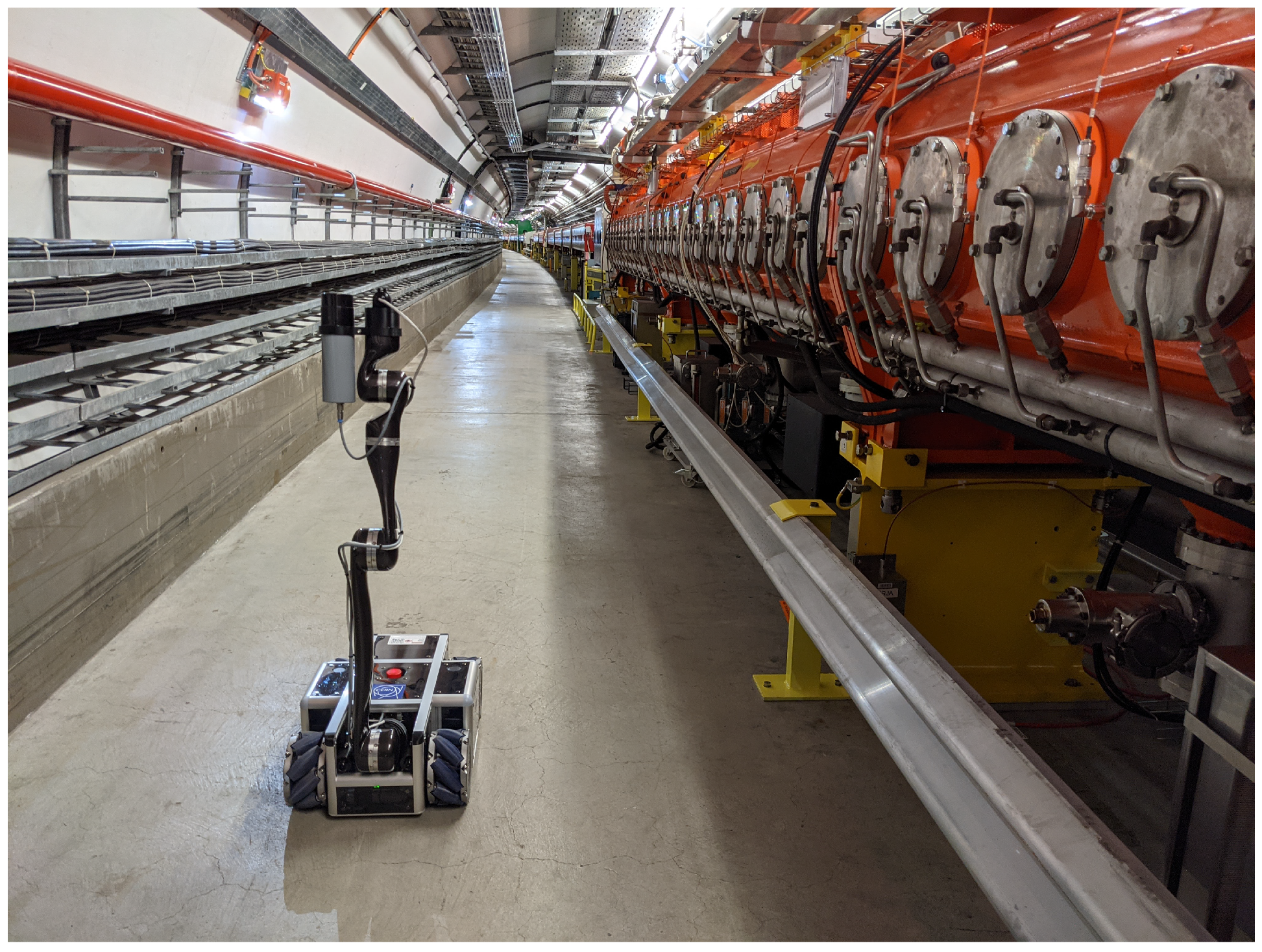
The result of the work presented in this paper is an omnidirectional robotic platform, whose first prototype still does not count all the required sensors for autonomous surveillance. As shown in Figure 10, a monitored surveillance was perform in the SPS accelerator by members of the robotic group of CERN. Throughout the tests, the operator remotely navigated the robotic platform from the control room. In this case, the operator had the information from the cameras; however, in future interventions a point cloud-based reconstruction system for three-dimensional environments will be available, thanks to the installed 3D LIDAR. This addition will help the operator and control to cross the gates along the tunnel. Due to the developed tests, it was tested that the robot design comply with the first, third and forth requirements of Section 1, which are related with surveillance time, robot speed and autonomy.

The robot was tested in its most critical point, this is, during crossing the section doors. As shown in Figure 11, the robot was able to cross it, complying in this way with the spatial requirements (the second requirement).

As explained in Section 1, the robot charges its batteries in one of the entrances of the SPS tunnel, where a charging station is available. In that moment, the robot folds the robotic arm over its top plate, as shown in Figure 12.

The kinematic and dynamic models were tested in a wide environment, obtaining the results shown in Figure 13. In that picture, the blue line represents the desired trajectory or ground truth, the red line represents the trajectory that the robot followed using the kinematic model, and the green line represents the trajectory using the dynamic model. The test was done within a wide environment, traveling a distance of approximately 90 m and changing the orientation in the meantime. It is calculated that the maximum error by the kinematic model during the given trajectory was 2.78 m and 5.1${}^{\circ }$, while the dynamic model reduced this error to 0.89 m and 0.45${}^{\circ }$.

7. Conclusions

In this paper, we have presented an original design of an omnidirectional robotic platform under very high spatial restrictions. The robot will perform the surveillance of the tunnel Super Proton Synchrotron, SPS, an accelerator of the European Organization for Nuclear Research, CERN. However, its applications are not only included in this environment, since it can be used in any installation where maneuverability is an essential requirement. Thanks to the compact design, this robot can deal with small spaces making use of the feature of setting horizontally the robotic arm that is mounted on it, together with the feature of folding the 3D LIDAR plate while crossing the doors and extract it while the surveillance. The robot is stably tested from a theoretical point of view, guaranteeing in this way the performance of the robot under foreseen circumstances. In addition, the final design of the robot is equipped with all the needed sensors and actuators, allowing not only the autonomous survey of the tunnel but also allowing it to be used in teleoperation tasks, where the end-effector tool may be changed.

The work presented represents a robot with very particular features. In the first place, the great distances that it must travel accompany the design of a large robotic platform, with the possibility of housing a large number of devices for measuring environmental variables and for intervention on the environment. However, the strict spatial restrictions that arise make it necessary to design a very small platform, even requiring physical robustness, high computing capacity and high load capacity for the portability of measurement and actuation devices. In addition, the design developed presents a novel ability to fold the robotic arm when crossing the doors, maintaining the stability of the small platform. In this way, the robot becomes the first interchangeable tool robot capable of performing tasks in large environments, such as tunnels, which have narrow passages 400 mm wide and 200 mm high.

The prototype of the platform has shown high capabilities to cross the small doors or narrow passages with the help of operators that control the motion, as well as good performance when the robot is driven to the charging station. The platform shows high maneuverability, allowing the robot to move within the narrow corridors and spaces that communicate the charging station with the tunnel.

Furthermore, to achieve proper control of the robot, the kinematic and dynamic models have been obtained. These models have been included in a user interface, which allows the operator to move the robot as desired, according to the information sent by the cameras and sensors.