
Experimental Verification of Real-Time Flow-Rate Estimations in a Tilting-Ladle-Type Automatic Pouring Machine


Abstract
:1. Introduction
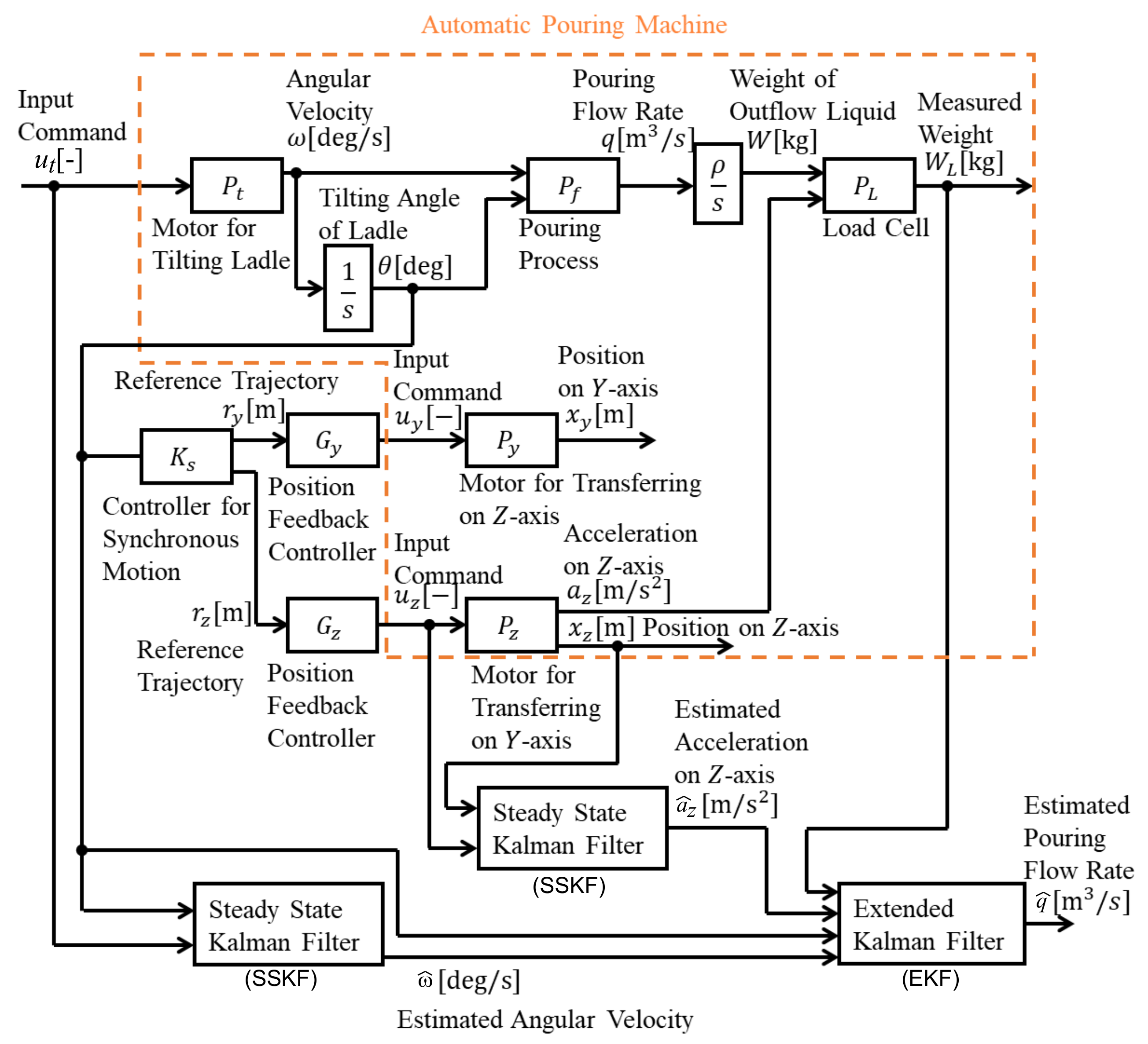
2. Automatic Pouring Machine
3. Mathematical Models of Pouring Motion
3.1. Motor Model for the Tilting Ladle
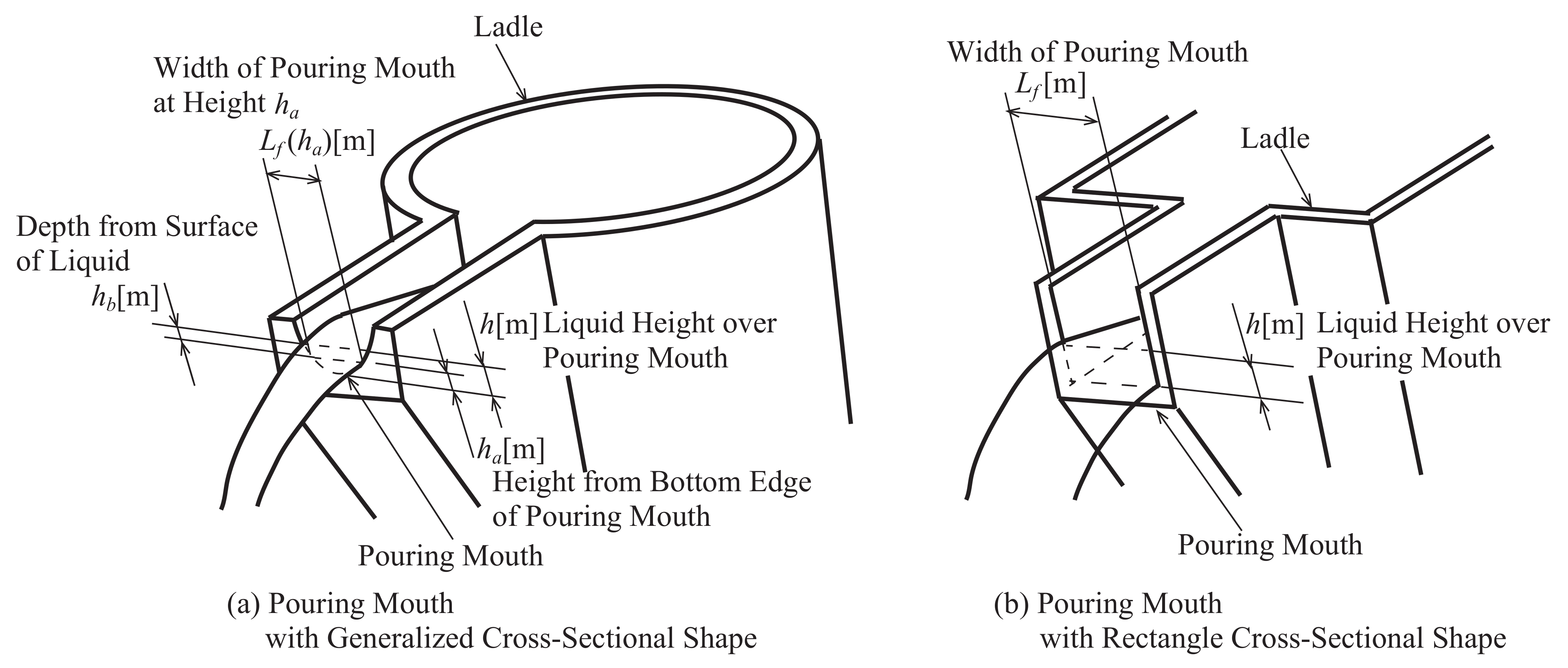
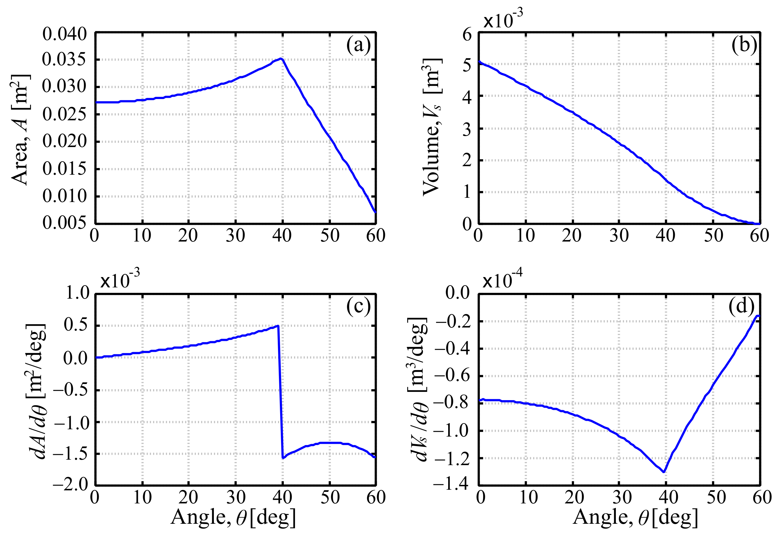
3.2. The Pouring Process Model
3.3. Load Cell Model
3.4. Motor Model for Transferring the Ladle on the y- and z-Axes
3.5. Synchronous Control for Transferring and Rotating the Ladle
4. Compensation of Measured Weight by Load Cell
5. Flow Rate Estimation by Decentralization of Kalman Filters
5.1. The Design of Flow Rate Estimation
- Predict
- Update
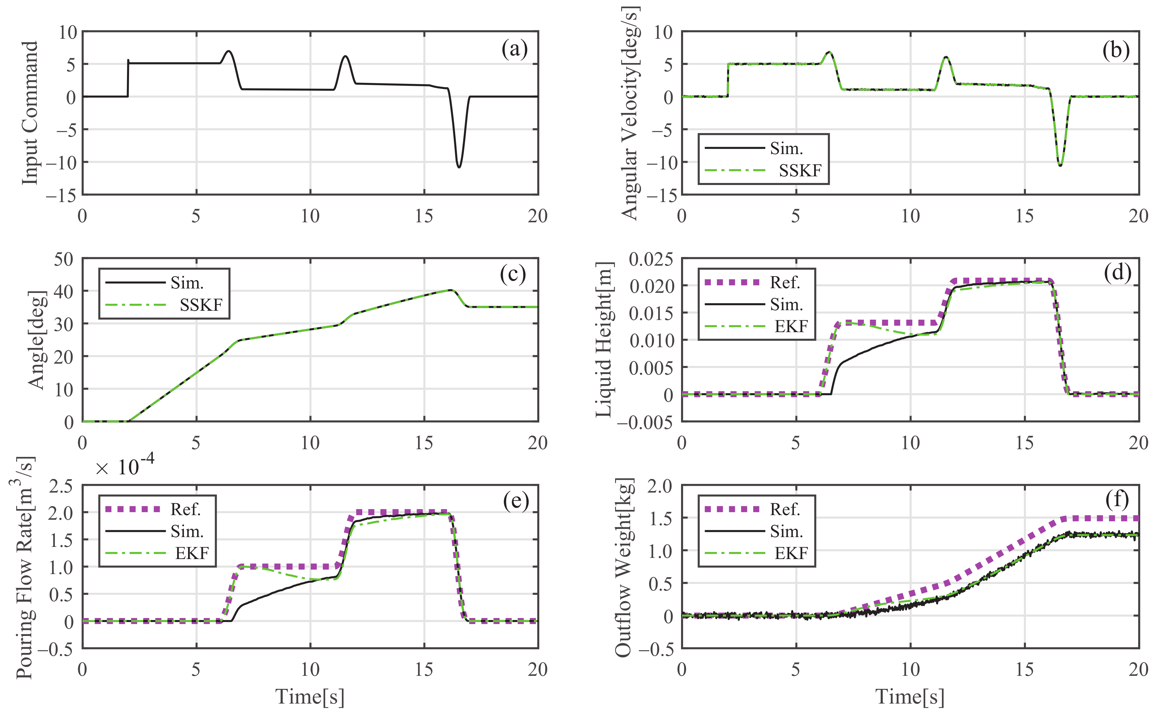
5.2. Simulations
6. Other Flow-Rate Estimation Methods for Comparison
6.1. Flow-Rate Estimation by Differentiating Load Cell Data
6.2. Flow-Rate Estimation Using a Visible Camera
7. Experimental Verifications
8. Conclusions
Author Contributions
Funding
Institutional Review Board Statement
Informed Consent Statement
Conflicts of Interest
Abbreviations
| CFD | Computational Fluid Dynamics |
| SSKF | Steady State Kalman Filter |
| EKF | Extended Kalman Filter |
| DKFs | Decentralization of Kalman Filters |
| DC | Direct Current |
| IAE | Integral Absolute Error |
| TV | Total Variation |
| mTV | Modified Total Variation |
References
- Lindsay, W. Automatic pouring and metal distribution system. Foundry Trade J. 1983, 10, 151–176. [Google Scholar]
- Terashima, K. Recent automatic pouring and transfer systems in foundries. Mater. Process Technol. 1998, 39, 1–8. (In Japanese) [Google Scholar]
- Neumann, E.; Trauzeddel, D. Pouring systems for ferrous applications. Foundry Trade J. 2002, 176, 23–24. [Google Scholar]
- Tiwari, P.; Kothawale, R.; Tadav, P. Semi automatic pouring system. Int. Res. J. Eng. Technol. 2017, 4, 2834–2837. [Google Scholar]
- Li, L.; Wang, C.; Wu, H. Research on kinematics and pouring law of a mobile heavy load pouring robot. Math. Probl. Eng. 2018, 2018, 1–13. [Google Scholar] [CrossRef]
- Watanabe, J.; Yoshida, K. Automatic pouring equipment for casting-Mel pore system. Ind. Heat. 1992, 29, 19–27. (In Japanese) [Google Scholar]
- Birkhold, M.; Friedrich, C.; Lechler, A. Automation of the casting process using a model-based NC architecture. IFAC-PapersOnLine 2015, 48, 195–200. [Google Scholar] [CrossRef]
- Yajima, T.; Noda, Y. Teaching-and-playback approach based on pouring flow rate in tilting-ladle-type pouring machine. In Proceedings of the 73rd World Foundry Congress, Cracow, Poland, 23–27 September 2018; pp. 137–138. [Google Scholar]
- Voss, T. Optimization and control of modern ladle pouring process. In Proceedings of the 73rd World Foundry Congress, Cracow, Poland, 23–27 September 2018; pp. 497–498. [Google Scholar]
- Yano, K.; Terashima, K. Supervisory control of automatic pouring machine. Control Eng. Pract. 2010, 18, 230–241. [Google Scholar] [CrossRef]
- Iwamoto, K.; Tokunaga, H.; Okane, T. Training support for pouring task in casting process using stereoscopic video see-through display. In Proceedings of the 2014 1st International Conference on Information Technology, Computer and Electrical Engineering, Semarang, Indonesia, 7–8 November 2014; pp. 497–498. [Google Scholar]
- Terashima, K.; Yano, K.; Sugimoto, Y.; Watanabe, M. Position control of ladle tip and sloshing suppression during tilting motion in automatic pouring machine. In Proceedings of the IFAC Symposium on Automation in Mining, Mineral and Metal Processing, Tokyo, Japan, 4–6 September 2001; pp. 229–234. [Google Scholar]
- Ito, A.; Tasaki, R.; Suzuki, M.; Terashima, K. Analysis and control of pouring ladle with weir for sloshing an volume-moving vibration in pouring cut-off process. J. Autom. Technol. 2017, 11, 645–656. [Google Scholar] [CrossRef]
- Tzamtzi, P.M.; Koumboulis, N.F. Sloshing control in tilting phases of the pouring process. Int. Sch. Sci. Res. Innov. 2007, 10, 3035–3042. [Google Scholar]
- Tzamtzi, P.M.; Koumboulis, N.F.; Skarpetis, G.M. On the Modelling and controller design for the outpouring phase of the pouring process. WSEAS Trans. Syst. Control 2009, 4, 11–20. [Google Scholar]
- Moriello, L.; Biagiotti, L.; Melchiorri, C.; Paoli, A. Control of liquid handling robotic systems: A feed-forward approach to suppress sloshing. In Proceedings of the 2017 IEEE International Conference on Robotics and Automation, Singapore, 29 May–3 June 2017. [Google Scholar] [CrossRef] [Green Version]
- Moriello, L.; Biagiotti, L.; Melchiorri, C.; Paoli, A. Manipulating liquids with robots: A sloshing-free solution. Control Eng. Pract. 2018, 78, 129–141. [Google Scholar] [CrossRef] [Green Version]
- Fukushima, R.; Noda, Y.; Terashima, K. Falling position and anti-sloshing control of liquid using automatic pouring robot. In Proceedings of the International PhD Foundry Conference, Brno, Czech Republic, 1–3 June 2009; pp. 1–10. [Google Scholar]
- Liang, H.; Li, S.; Ma, X.; Hendrich, N.; Gerkmann, T.; Zhang, J. Making sense of audio vibration for liquid height estimation in robotic pouring. In Proceedings of the 2019 IEEE/RSJ International Conference on Intelligent Robots and Systems, Macau, China, 3–8 November 2019. [Google Scholar] [CrossRef] [Green Version]
- Rozo, L.; Jimenez, P.; Torras, C. Force-based robot learning of pouring skills using parametric hidden Markov models. In Proceedings of the 9th International Workshop on Robot Motion and Control, Kuskin, Poland, 3–5 July 2013. [Google Scholar] [CrossRef] [Green Version]
- Kuriyama, Y.; Yano, K.; Nishido, S. Optimization of pouring velocity for aluminium gravity casting. In Fluid Dynamics, Computational Modeling and Applications; IntechOpen: London, UK, 2012; pp. 575–588. [Google Scholar]
- Noda, Y.; Terashima, K. Modeling and feedforward flow rate control of automatic pouring system with real ladle. J. Robot. Mechatronics 2007, 19, 205–211. [Google Scholar] [CrossRef]
- Noda, Y.; Fukushima, R.; Terashima, K. Monitoring and control system to falling position of outflow liquid in automatic pouring robot. In Proceedings of the IFAC 13th Symposium on Automation in Mining, Mineral and Metal Processing, Cape Town, South Africa, 2–4 August 2010; pp. 13–18. [Google Scholar] [CrossRef]
- Ito, A.; Noda, Y.; Tasaki, R.; Terashima, K. Outflow liquid falling position control considering lower pouring mouth position with collision avoidance for tilting-type automatic pouring machine. Mater. Trans. 2017, 58, 485–493. [Google Scholar] [CrossRef] [Green Version]
- Sueki, Y.; Noda, Y.; Suzuki, M.; Ohta, K. Optimization of ladle position to minimize spilled liquid from pouring basin in automatic pouring machine. J. Jpn. Foundry Eng. Soc. Jpn. 2018, 90, 107–117. (In Japanese) [Google Scholar]
- Sueki, Y.; Noda, Y. Optimal positioning of ladle in automatic pouring machine in consideration of pouring liquid accurately into sprue. In Proceedings of the IEEE International Conference on Advanced Intelligent Mechatronics, Munich, ND, USA, 3–7 July 2017; pp. 897–903. [Google Scholar]
- Noda, Y.; Terashima, K. State estimation of automatic pouring system with load cell in casting process. In Proceedings of the SICE Annual Conference 2008, Tokyo, Japan, 20–22 August 2008; pp. 1548–1551. [Google Scholar]
- Noda, Y.; Terashima, K. Estimation of flow rate in automatic pouring system with real ladle used in industry. In Proceedings of the ICROS-SICE International Conference 2009, Fukuoka, Japan, 18–21 August 2009; pp. 354–359. [Google Scholar]
- Noda, Y.; Birkhold, M.; Terashima, K.; Sawodny, O.; Verl, A. Flow rate estimation using unscented Kalman filter in automatic pouring machine. In Proceedings of the SICE Annual Conference 2011, Tokyo, Japan, 13–18 September 2011; pp. 769–774. [Google Scholar]
- Noda, Y.; Zeitz, M.; Sawodny, O.; Terashima, K. Flow rate control based on differential flatness in automatic pouring robot. In Proceedings of the 2011 IEEE International Conference on Control Applications, Denver, CO, USA, 28–30 September 2011; pp. 1468–1475. [Google Scholar]
- Noda, Y.; Terashima, K. Simplified flow rate estimation by decentralization of Kalman filters in automatic pouring robot. In Proceedings of the SICE Annual Conference 2012, Akita, Japan, 20–23 August 2012; pp. 1465–1470. [Google Scholar]
- Noda, Y.; Sueki, Y. Implementation and experimental verification of flow rate control based on differential flatness in a tilting-ladle-type automatic pouring machine. Appl. Sci. 2019, 9, 1978. [Google Scholar] [CrossRef] [Green Version]
- Shinohara, K.; Morimoto, H. Development of automatic pouring equipment. J. Soc. Automot. Eng. Jpn. 1992, 46, 79–85. (In Japanese) [Google Scholar]
- Yamaguchi, A.; Atkeson, C. Stereo vision of liquid and particle flow for robot pouring. In Proceedings of the 2016 IEEE-RAS 16th International Conference on Humanoid Robots, Cancun, Mexico, 15–17 November 2016; pp. 1173–1180. [Google Scholar]
- Schenck, C.; Fox, D. Visual closed-loop control for pouring liquids. In Proceedings of the 2017 IEEE International Conference on Robotics and Automation, Singapore, 29 May–3 July 2017. [Google Scholar] [CrossRef] [Green Version]
- Do, C.; Burgard, W. Accurate Pouring with an Autonomous robot using an RGB-D camera. Intell. Auton. Syst. 2019, 15, 210–221. [Google Scholar] [CrossRef]
- Kennedy, M., III; Queen, K.; Thakur, D.; Kumar, V. Precise dispensing of liquids using visual feedback. In Proceedings of the 2017 IEEE/RSJ International Conference on Intelligent Robots and Systems, Vancouver, BC, Canada, 24–28 July 2017. [Google Scholar] [CrossRef]
- Suzuki, M.; Yang, Y.; Noda, Y.; Terashima, K. Sequence control of automatic pouring system. In Proceedings of the 10th Asian Foundry Congress, Aichi, Japan, 21–24 May 2008; pp. 88–92. [Google Scholar]
- Kabasawa, N.; Noda, Y. Model-based flow rate control with online model parameters identification in automatic pouring machine. Robotics 2021, 10, 39. [Google Scholar] [CrossRef]
- Skogestad, S. Simple Analytic Rules for Model Reduction and PID Controller Tuning. J. Process Control 2003, 13, 291–309. [Google Scholar] [CrossRef] [Green Version]
- Huba, M.; Vrancic, D. Extending the Model-Based Controller Design to Higher-Order Plant Models and Measurement Noise. Symmetry 2021, 13, 798. [Google Scholar] [CrossRef]


| Estimation Method | Tilting Angle Error at Start | Tilting Angle Error at Start |
|---|---|---|
| to Liquid Outflow +0 deg | to Liquid Outflow +3 deg | |
| DKFs with Covariance of Process Noise in Equation (37) | ||
| DKFs with Covariance of Process Noise in Equation (46) | ||
| Differentiating Load Cell Data | ||
| Visible Camera |
Publisher’s Note: MDPI stays neutral with regard to jurisdictional claims in published maps and institutional affiliations. |
© 2021 by the authors. Licensee MDPI, Basel, Switzerland. This article is an open access article distributed under the terms and conditions of the Creative Commons Attribution (CC BY) license (https://creativecommons.org/licenses/by/4.0/).
Share and Cite
Sueki, Y.; Noda, Y. Experimental Verification of Real-Time Flow-Rate Estimations in a Tilting-Ladle-Type Automatic Pouring Machine. Appl. Sci. 2021, 11, 6701. https://doi.org/10.3390/app11156701
Sueki Y, Noda Y. Experimental Verification of Real-Time Flow-Rate Estimations in a Tilting-Ladle-Type Automatic Pouring Machine. Applied Sciences. 2021; 11(15):6701. https://doi.org/10.3390/app11156701
Chicago/Turabian StyleSueki, Yuta, and Yoshiyuki Noda. 2021. "Experimental Verification of Real-Time Flow-Rate Estimations in a Tilting-Ladle-Type Automatic Pouring Machine" Applied Sciences 11, no. 15: 6701. https://doi.org/10.3390/app11156701