Implementation of Adaptive Real-Time Camouflage System in Visible-Light Band

Featured Application

In order to meet the camouflage requirements for various applications, with different climates conditions of full-time, this paper proposes an adaptive real-time camouflage control system in the visible light band. The sensor technology, image processing technology, and display technology are well combined by this camouflage control system.

Abstract

This paper presents an adaptive camouflage system in visible band, featuring a dominant color feature-matching algorithm and pulse width modulation (PWM)-based display driving circuit. The control system consists of three parts, namely, the background sensing part, the central processing part, and the physical driving waveform generation part. Images of the local environment are sampled by the background sensing part, and then the dominant color feature matching algorithm is conducted to select a proper camouflage image that matches the local environment. Consequently, the cholesteric liquid crystals (CLCs) display using amplitude adjustable AC voltage, which is modulated by the physical driving waveform generation unit. The experimental results show that the matching degree of the proposed algorithm was 2.47 times that of the conventional hue (H), saturation (S), and value (V) histogram camouflage evaluation method, while the output peak wavelength of the reflective band can be adjusted from 604 to 544 nm according to the ambient color profile.

1. Introduction

Camouflage technology attracts widespread attention, while adaptive camouflage system for visible-light band is still a great challenge. Conventionally, camouflage effects are achieved using nets and painted patterns with fixed color and geometry. However, these camouflage approaches are prone to fail in mobile environments for real-time applications [1,2]. For better camouflage effects, it is important to sense light-bands of the local environments, as well as to adjust the appearance of the target in color and pattern [3]. Xie et al. proposed a camouflage control system on the basis of field-programmable gate array (FPGA) platform. Images of external environments are captured by the charge coupled device (CCD) camera, and then are converted to RGB digital signals. Then, the electro-chromic device is driven through the FPGA platform, which is connected with CCD [4]. Pezeshkian et al. proposed an adaptive camouflage platform on the basis of electronic paper panels [5].

The sensor technology, image processing technology [6], and display technology are well combined by the real-time control system. Overall, there are three consecutive steps for real-time camouflage system: (i) sampling the local environment using cameras, (ii) generating the camouflage pattern similar to the local environment, and (iii) displaying the proper camouflage image. The second step aims at finding a particular camouflage image that possesses the highest similarity with the environment. Conventionally, the digital images of the target and environment are converted into grayscale formats, and then grayscale histograms are calculated and compared for calibrations. Although the conventional camouflage-synthesis method is commonly used for compact representation and reduced complexity, there are some problems to be solved, such as inefficiency in representing images with few dominant colors and low image registration accuracy [7]. For the third step, it is important to choose proper display devices to mimic the local environment. However, the traditional display devices are heavily dependent on backlight modules, which bring difficulty to adjust the color and textures in real time [4].

In this paper, we present a dominant color feature-matching algorithm for image matching in the HSL space. The proposed algorithm performs better than the method of grayscale histogram calculation in terms of complexity, matching efficiency, and accuracy. The reflective-type cholesteric liquid crystals (CLCs) were chosen as display device, avoiding the use of backlight module. The rest of this paper is organized as follows. The second section presents the architecture of an adaptive camouflage system, which is based on dominant color feature matching algorithm and CLC display. In the third section, the matching result between the camouflage image and local environment is evaluated. Finally, conclusions are given in the fourth section.

2. Methods

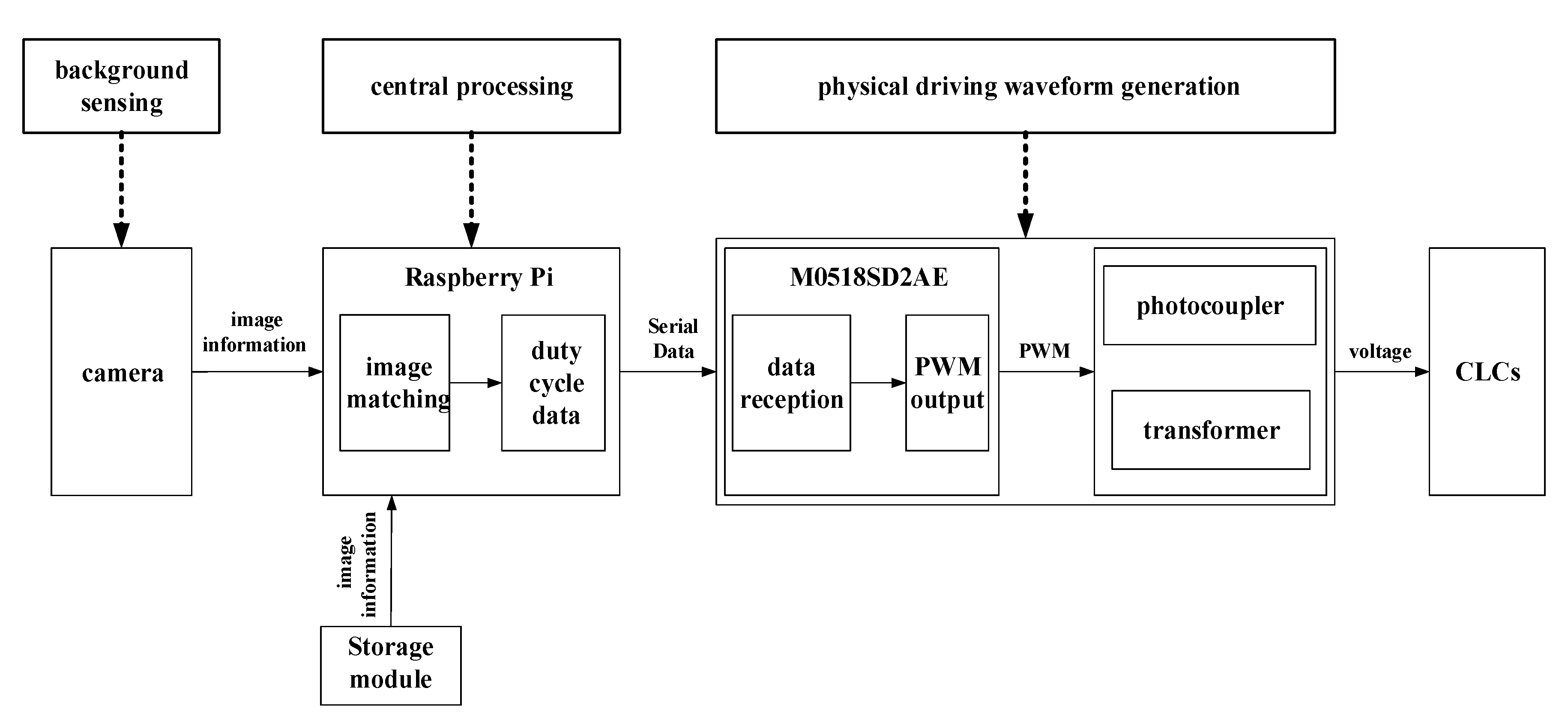
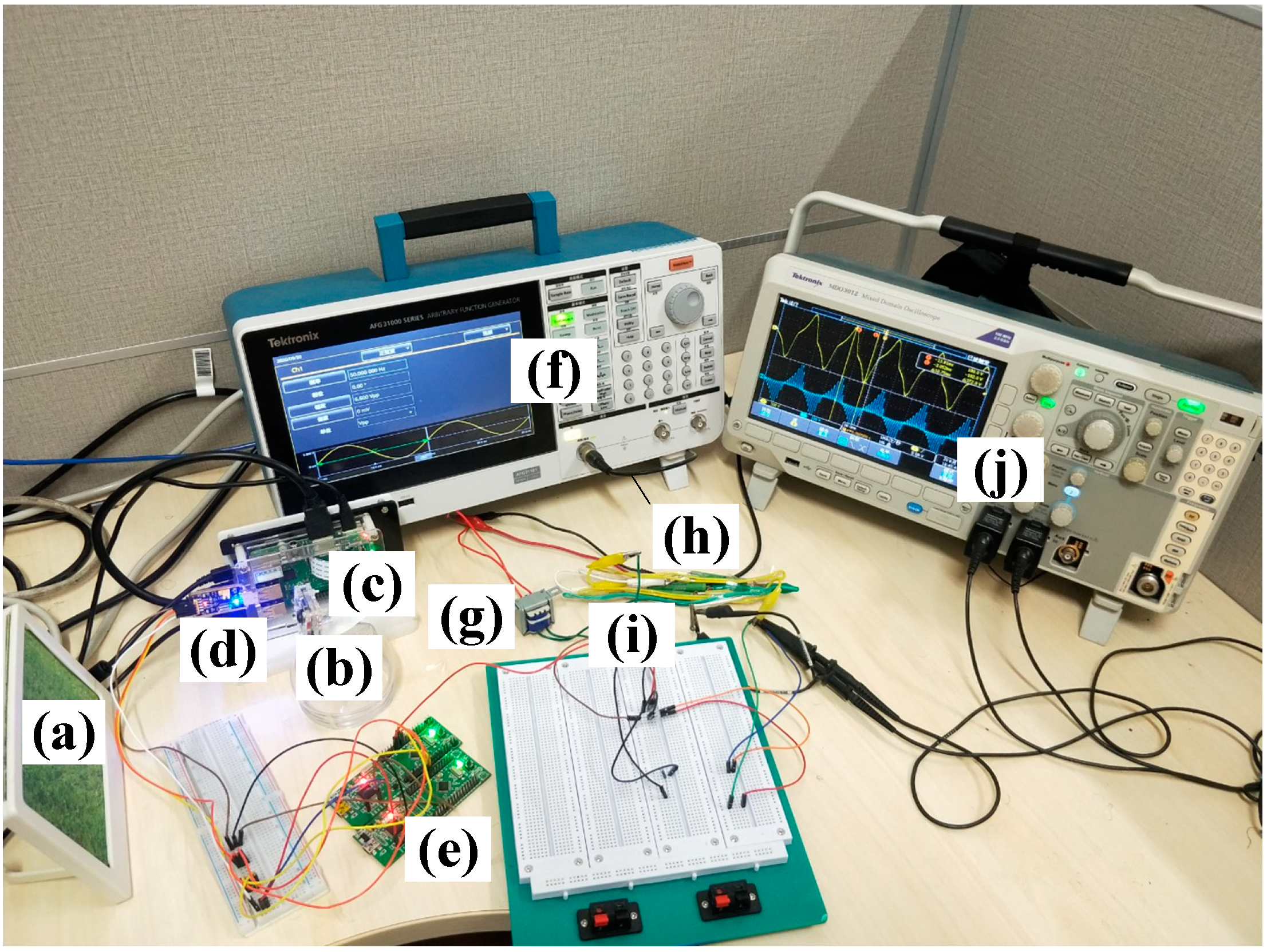
2.1. A Visible-Band Adaptive Camouflage System

Figure 1 shows the block diagram of the proposed camouflage control system, which consists of the background sensing part, the central processing part, and the physical driving waveform generation part. In the background sensing unit, the camera (PI NOIR CAMERA V2) samples images of the environment. The central processing unit is based on a Raspberry Pi embedded board, used to conduct the dominant color feature matching algorithm, as well as to output the encoded signal to M0518SD2AE MCU through USB-TTL chip (CH341T). The physical driving waveform generation outputs adjustable AC voltage with an amplitude of 0–250 V (RMS value), which tunes the photoelectric characteristics of the CLCs devices.

2.2. The Dominant Color Feature-Matching Algorithm

Here, a new algorithm for color matching is presented. In order to evaluate the similarity metric between the target and the environment, we calculated the distance between dominant colors using correlation coefficient.

We exploited hue, saturation, and luminance (HSL) color space, as H, S, an L components can be individually controlled with an intuitive color representation to the way humans perceive colors [8]. In this method, the colors are divided into 12 types of hue (H), 2 types of saturation (S), and 3 types of luminance (L). Counting the number of pixels in the divided color gamut interval, in which the top five colors with the maximum number of pixels are used as the dominant colors, is sufficient in order to describe the total color information [9].

The steps we proposed to implement the dominant color feature matching algorithm are as follows:

(1)

Extract the RGB values (R, G, B) of each pixel in the local environmental image.

(2)

Transform the RGB values (R, G, B) of each pixel in the local environment image into the HSL space to obtain the corresponding HSL values (H, S, L). The conversion formula of RGB and HSL color space is as follows [10]:

$$H=\{\begin{array}{c}\arccos \left\{\frac{(R-G)=(R-B)}{2\sqrt{{(R-G)}^2+(R-B)(G-B)}}\right\}R\ne G\mathrm{and}R\ne B\\ 2\pi -\arccos \left\{\frac{\left(R-G\right)+\left(R-B\right)}{2\sqrt{{\left(R-G\right)}^2+\left(R-B\right)\left(G-B\right)}}\right\}B>G\end{array}$$

(1)

$$S=1-3÷\left(R+G+B\right)\times \min \left(R,G,B\right)$$

(2)

$$L=\left(R+G+B\right)/3$$

(3)

where $H\in [0°, 360°]$, $L,S\in [0, 1]$.

(1)

Obtain the dominant color feature matrix of the environment image according to the HSL color gamut interval. The dominant colors are expressed as the dominant colors feature matrix, which contains 26 elements. Each element corresponds to the sum of pixels in the divided color gamut interval, as shown in

Table 1. The corresponding relationship between elements of feature matrix and color.

Element	H	S	L	Color
F[0]	(345°,360°] ∪ (360°,15°]	(0,0.5]	[0,1]	red
F[1]	(345°,360°] ∪ (360°,15°]	(0.5,1]	[0,1]	red
F[2]	(15°,45°]	(0,0.5]	[0,1]	orange
F[3]	(15°,45°]	(0.5,1]	[0,1]	orange
F[4]	(45°,75°]	(0,0.5]	[0,1]	yellow
F[5]	(45°,75°]	(0.5,1]	[0,1]	yellow
F[6]	(75°,105°]	(0,0.5]	[0,1]	flavo-green
F[7]	(75°,105°]	(0.5,1]	[0,1]	flavo-green
F[8]	(105°,135°]	(0,0.5]	[0,1]	green
F[9]	(105°,135°]	(0.5,1]	[0,1]	green
F[10]	(135°,165°]	(0,0.5]	[0,1]	bluish green
F[11]	(135°,165°]	(0.5,1]	[0,1]	bluish green
F[12]	(165°,195°]	(0,0.5]	[0,1]	cyan
F[13]	(165°,195°]	(0.5,1]	[0,1]	cyan
F[14]	(195°,225°]	(0,0.5]	[0,1]	cyan-blue
F[15]	(195°,225°]	(0.5,1]	[0,1]	cyan-blue
F[16]	(225°,255°]	(0,0.5]	[0,1]	blue
F[17]	(225°,255°]	(0.5,1]	[0,1]	blue
F[18]	(255°,285°]	(0,0.5]	[0,1]	bluish violet
F[19]	(255°,285°]	(0.5,1]	[0,1]	bluish violet
F[20]	(285°,315°]	(0,0.5]	[0,1]	purple
F[21]	(285°,315°]	(0.5,1]	[0,1]	purple
F[22]	(315°,345°]	(0,0.5]	[0,1]	purplish red
F[23]	(315°,345°]	(0.5,1]	[0,1]	purplish red
F[24]	0°	(0,0.5]	[0,1]	black
F[25]	0°	(0.5,1]	[0,1]	white

.

(2)

Normalize the dominant colors feature matrix, which means to divide F[i] by the total number of pixels, with F[i] being the number of times a pixel having color i appears in the image.

(3)

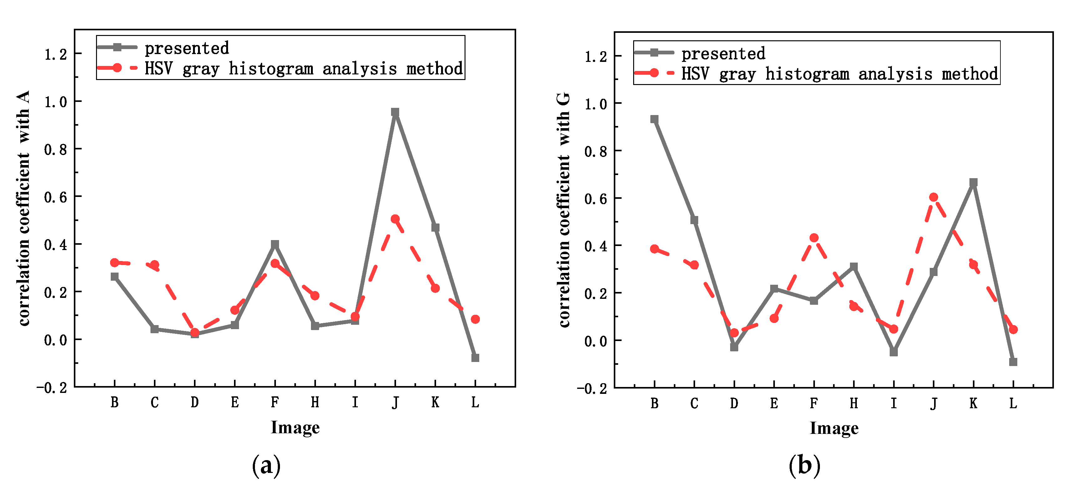
Obtain the camouflage image with the highest similarity to the environment image. On the basis of the optimal matching theory, the similarity measure of the camouflage image and the target image can be computed by the correlation coefficient. Then, the retrieved result is ranked according to the value of similarity. The formula of correlation coefficient is as follows [11]:

$$r=\frac{{\displaystyle \sum _i(x_i-x_m)}(y_i-y_m)}{\sqrt{{\displaystyle \sum _i{(x_i-x_m)}^2}}\sqrt{{\displaystyle \sum _i{(y_i-y_m)}^2}}},$$

(4)

where $x_i$ is the intensity of the $i_{th}$ pixel in environmental image, $y_i$ is the intensity of the $i_{th}$ pixel in camouflage image, $x_m$ is the mean intensity of environmental image, and $y_m$ is the mean intensity of camouflage image.

It is worthwhile comparing the proposed dominant color feature matching algorithm and other relevant counterparts such as the automatic image allocation method proposed by Nejad et al. [12], which features image feature value extraction, dimensionality reduction, classification, and evaluation. Compared with traditional methods, the accuracy and sensitivity can be improved by the proposed algorithm.

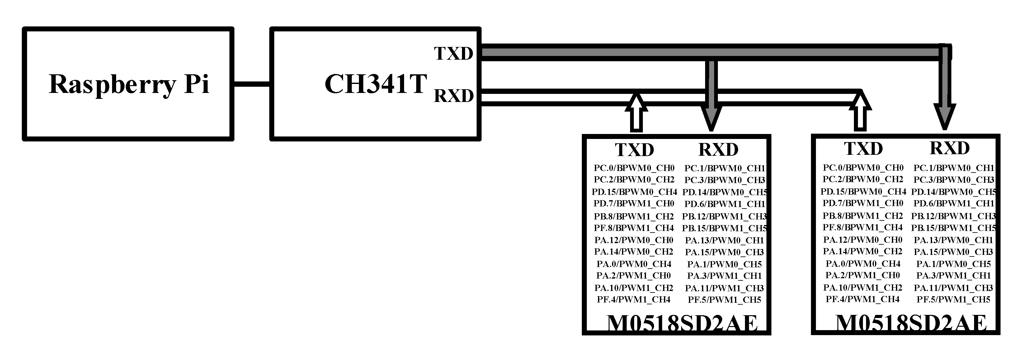
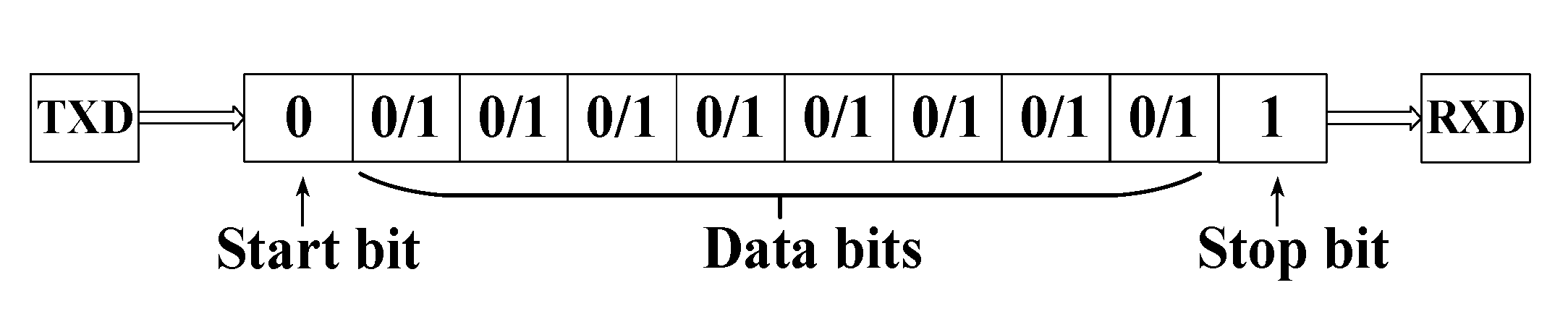
2.3. PWM Driving Circuit for the CLC Display

For system simplicity, pulse width modulation (PWM), i.e., brightness being tuned by the ON duty ratio of the input digital video signal, is used [13,14]. The PWM drive is essentially compatible with the operation of the large-area display, such as active-matrix organic light emitting diode (AMOLED) display [15,16,17]. Before the converting of the brightness information to the ON duration of the PWM driving signal, the data transmission between the Raspberry Pi and the M0518SD2AE MCU have to firstly be realized. Figure 2 shows the data transmission between the Raspberry Pi and the M0518SD2AE MCU through the USB-TTL Communication. When the baud rate parameter is set to 9600, the data sequence sent by the host Raspberry Pi is shown in Figure 3. M0518SD2AE receives or transmits data in the interrupt subroutine [18].

According to the opt-electrical characteristic of the adopted CLCs display, a high-voltage modulation circuit with an amplitude of 250 V is required. The schematic diagram of the high voltage RMS amplitude modulation circuit is shown in Figure 4. In the implemented high voltage modulation circuit, a high-voltage AC boosted by a transformer is connected to the photo-coupler ELM3064 through a 400 Ω high power resistor. The high-voltage AC can be conducted or cut off with the ON or OFF duration of the PWM driving signal.

3. Results and Discussions

3.1. Camouflage Image Matching Results

In order to verify the feasibility of the proposed dominant color feature matching algorithm, we carried out experiments using grassland and jungle pictures as local environment images to be matched.

According to the steps of realizing the dominant color feature matching method, the grass image shown in Figure 5A was used as the environment image and the dominant color matrix was F[0, 0, 0, 0, 0, 247, 9479, 3218, 44,798, 0, 0, 0, 0, 0, 0, 0, 0, 0, 0, 0, 0, 0, 0, 0, 0, 6388], as shown in

Table 2. The correlation coefficient between environmental image and camouflage images.

Image	The Dominant Color Feature Matrix	Correlation Coefficient with A	Correlation Coefficient with G
A	F[0, 0, 0, 0, 0, 247, 9479, 3218, 44,798, 0, 0, 0, 0, 0, 0, 0, 0, 0, 0, 0, 0, 0, 0, 0, 0, 6388]
G	F[0, 0, 0, 0, 0, 0, 4208, 58,147, 19,464, 6408, 0, 0, 0, 0, 0, 0, 0, 0, 0, 0, 0, 0, 0, 0, 0, 8980]
B	F[0, 0, 0, 0, 0, 12,500, 2181, 36,468, 10,008, 0, 0, 0, 0, 0, 0, 0, 0, 0, 0, 0, 0, 0, 0, 0, 0, 1018]	0.26235	0.93230
C	F[0, 0, 0, 7239, 0, 79,782, 0, 59,143, 0, 0, 0, 6142, 0, 0, 0, 0, 0, 5309, 0, 0, 0, 0, 0, 0, 0, 0]	−0.04206	0.50677
D	F[0, 136,885, 0, 11,919, 0, 3877, 0, 0, 0, 0, 0, 0, 0, 0, 0, 0, 0, 0, 0, 0, 0, 0, 0, 0, 0, 59,333]	−0.02123	−0.02930
E	F[0, 0, 0, 0, 0, 133,677, 0, 41,677, 0, 20,995, 0, 19,027, 0, 1228, 0, 0, 0, 0, 0, 0, 0, 0, 0, 0, 0, 0]	−0.05872	0.21728
F	F[0, 0, 0, 0, 0, 0, 0, 0, 43,362, 57,120, 24,460, 0, 32,468, 0, 0, 0, 0, 0, 0, 0, 0, 0, 0, 0, 0, 79,799]	0.39913	0.16673
H	F[0, 0, 0, 0, 0, 0, 0, 6736, 160, 21,005, 6302, 0, 0, 0, 0, 0, 0, 0, 0, 0, 0, 0, 0, 0, 0, 467]	−0.05491	0.30998
I	F[0, 16,895, 0, 160,235, 0, 67,242, 0, 7454, 0, 0, 0, 0, 0, 0, 0, 0, 0, 0, 0, 0, 0, 0, 0, 0, 0, 743]	−0.07727	−0.05059
J	F[0, 0, 0, 0, 0, 1, 630, 22, 77,990, 0, 0, 0, 0, 0, 0, 0, 0, 0, 0, 0, 0, 0, 0, 0, 0, 28,157]	0.95458	0.28831
K	F[0, 0, 0, 0, 0, 24,994, 0, 27,285, 25,322, 23,557, 0, 3201, 0, 0, 0, 0, 0, 0, 0, 0, 0, 0, 0, 0, 0, 0]	0.46870	0.66638
L	F[0, 0, 0, 0, 0, 0, 0, 0, 0, 0, 0, 0, 0, 0, 0, 125,496, 109,914, 63,076, 0, 9809, 0, 0, 0, 0, 0, 41,875]	−0.07857	−0.09224

, which means that yellow, flavo-green, and white were the dominant colors in the grass image. It can be seen that the environment image was weakly correlated with Figure 5B,F and was moderately correlated with Figure 5K. The similarity between the grass image and Figure 5J was the highest, which meant the grass image had the highest matching degree with Figure 5J. In the same way, for the jungle environment image, the most matching camouflage image was Figure 5B.

3.2. Camouflage Assessment

The typical method for camouflage matching is the classical color-histogram method. Wei et al. proposed a method for camouflage matching based on HSV gray histogram analysis [19]. In this paper, we illustrated the performance of the new algorithm we proposed by comparing it to the camouflage matching method based on HSV gray histogram.

According to the steps of realizing the camouflage matching method based on HSV gray histogram analysis, we calculated the similarity as shown in

Table 3. The camouflage matching method based on HSV gray histogram analysis.

Image	A				G
	H	S	V	Mean Correlation	H	S	V	Mean Correlation
B	0.8253	−0.0327	0.1054	0.3211	0.8496	0.0998	0.2053	0.3849
C	0.5136	−0.3520	−0.0715	0.3124	0.5500	0.0386	0.3637	0.3174
D	−0.0293	−0.0252	−0.0291	0.0278	−0.0343	0.0435	−0.0149	0.0309
E	0.0319	−0.1280	0.2056	0.1218	0.1719	0.0796	0.0251	0.0922
F	0.1684	0.7182	0.0666	0.3177	0.2446	0.8335	0.2185	0.4322
H	−0.0352	0.0908	0.4214	0.1825	0.1339	−0.0017	0.2905	0.1420
I	0.1420	−0.1069	0.0357	0.0948	0.0625	0.0434	0.0354	0.0471
J	0.6833	0.7683	0.0620	0.5045	0.4542	0.7918	0.5634	0.6031
K	0.5815	0.0347	0.0237	0.2133	0.6399	0.1879	0.1273	0.3184
L	−0.0418	−0.0205	0.1883	0.0835	−0.0489	−0.0476	0.0386	0.0450

. The average correlations between the grass image and camouflage images were 0.3211, 0.3124, 0.0278, 0.1218, 0.3177, 0.1825, 0.0948, 0.5045, 0.2133, which means that the camouflage image with the highest degree of matching with the grass image was Figure 5J. Similarly, the camouflage image with the highest degree of matching with the jungle image was Figure 5B. The results of the camouflage effect evaluation method based on HSV gray histogram analysis were the same as the dominant color feature matrix matching method proposed in this paper.

For the comparison of the accuracy of image matching, the optimal matching degree is defined to be dispersion of the correlation coefficient, and its calculation formula is as follows:

$$S=\sqrt{\frac{1}{N-1}{\displaystyle \sum _{i=1}^N{(\left|x_{\max }\right|-\left|x_i\right|)}^2}}$$

(5)

where $x_i$ is the value of the correlation coefficient, and $x_{\max }$ is the maximum value in the correlation coefficient.

For the grass and jungle background, the optimal matching degrees can be obtained as 0.7666 and 0.6671, respectively, by the dominant color feature matching method. Using the camouflage matching method based on HSV histogram, we found the optimal matching degrees to be 0.3182 and 0.2677, respectively. The optimal matching degree of the method proposed in this paper was 2.40 times that of the HSV gray histogram analysis method on average, which improved the confidence and accuracy of camouflage matching, as shown in Figure 6.

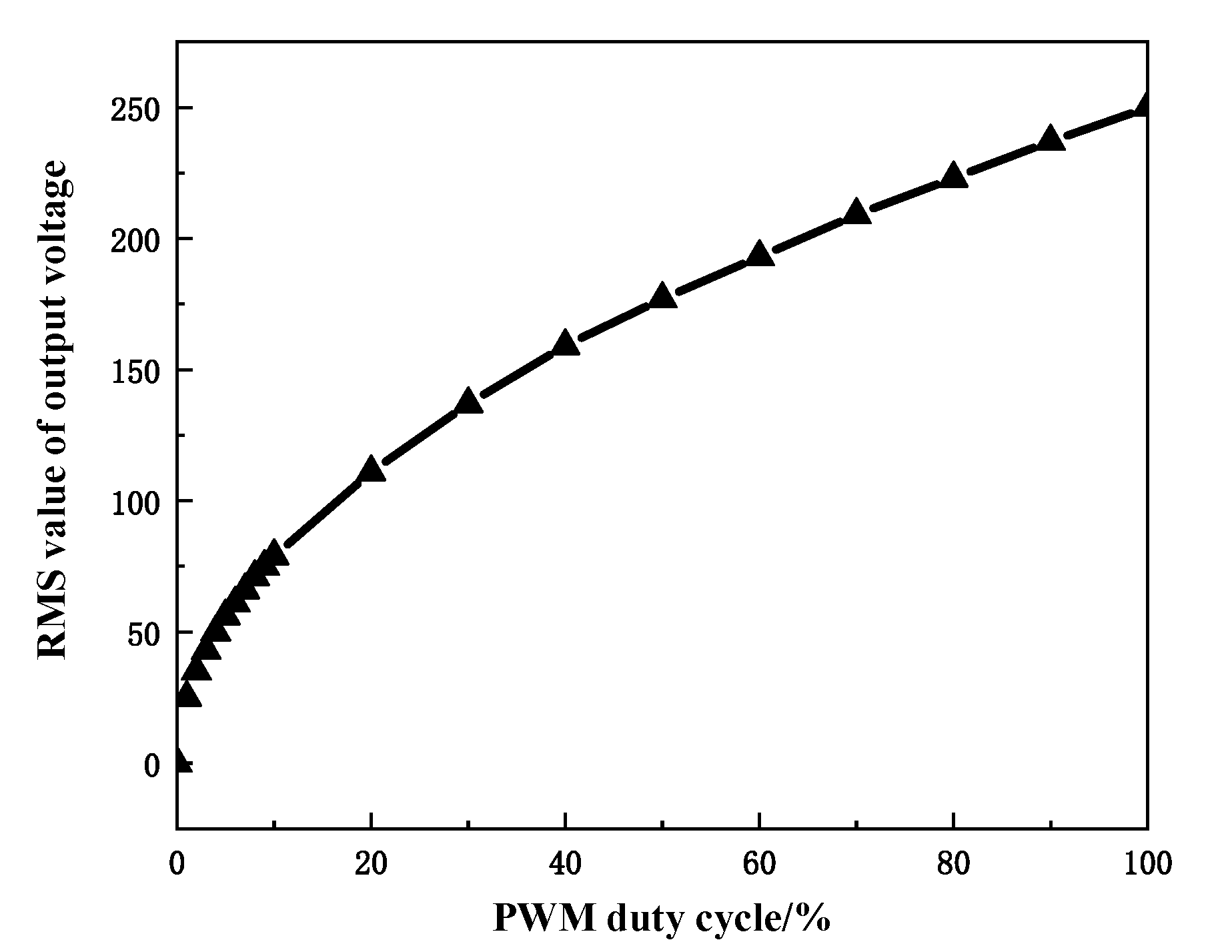
3.3. Results of PWM Signals

After the serial port configuration, the Raspberry Pi sends data, and the pulseview tool is used to connect the TXD pin of CH341T to capture data sent by the Raspberry Pi. Figure 7 shows that the captured data sent by the Raspberry Pi contained one start bit, eight data bits, and one stop bit.

In this study, the host Raspberry Pi was connected with two M0518SD2AE MCUs, as shown in Figure 8. The first slave M0518SD2AE MCU outputted the PWM signals with duty ratios of 10%, 20%, 30%, and 40%, as shown in D0, D2, D4, and D6, respectively, and the second slave M0518SD2AE MCU outputted the signals of D1, D3, D5, and D7, respectively. Each M0518SD2AE MCU can only output 24 PWM channels, and therefore multiple slaves are required to work together when displaying a complete camouflage image.

Figure 9 shows the input and output signals of high-voltage modulation circuit. The high-voltage AC can be conducted or cut off using the PWM driving signal. The photo-coupler isolates the control circuit from the high voltage electrodes to suppress interfaces.

Figure 10 shows the relationship between the duty cycle and RMS value of output voltage. After curve fitting, the relationship between output voltage and PWM duty cycle is expressed as

$$V=\{\begin{array}{c}23.27+5.8d-0.07d^2+3.62d^3 0<d\le 100\\ 0 d=0\end{array}$$

(6)

where $V$ is the output voltage RMS, and $d$ is the PWM duty ratio.

Figure 11 shows the movement of the reflection band of the CLCs under different voltages. The peak wavelength of the reflective band of CLCs was shifted from 604 to 544 nm with the voltage tuned from 0 to 250 V. After taking the environment image, the physical driving waveform generation part outputs the corresponding voltage signal to make the CLC device display the similar color with the environment for the purpose of camouflage.

Figure 12 shows the adaptive camouflage system, which includes environmental images (grass images), cameras, Raspberry Pi, M0518SD2AE MCU, transformer, photo-coupler ELM3064, signal generator, and oscilloscope. The camera (PI NOIR CAMERA V2) captures the grass image. After image acquisition and matching, the host Raspberry Pi transmits the PWM duty cycle signal to the two M0518SD2AE MCUs to output PWM signals through USB-TTL(CH341T) unit. The AC voltage signal with a frequency of 5 Hz and an amplitude of 3.3 V is provided by signal generator (AFG31000). The high-voltage AC voltage with the maximum RMS value of 250 V is generated by a transformer, and then a modulated 0–250 V RMS amplitude adjustable AC voltage is realized by the photo-coupler ELM3064. The 0–250 V output signal is collected by oscilloscope (MDO3012).

Table 4. The comparisons of system performance.

System	Platform	Camouflage Match	Response Time	Response Wavelength	Anti-Interference Ability
This work	Raspberry Pi	High accuracy	1.17s	604~544 nm	Stable
[4]	FPGA	N.A.	N.A.	560~580 nm	Susceptible to reflected light

shows the comparisons of system performance. The response time of the proposed system is reduced to 1.71 s, while a wider response wavelength range, stronger anti-interference ability can also be obtained.

4. Conclusions

In this paper, an adaptive optical camouflage control system design is demonstrated. The control system consists of three parts: background sensing, central processing, and physical driving waveform generation. In the central processing unit, a dominant color feature matching algorithm for image matching in the HSL space is proposed. Experimental results showed that the matching index of the proposed matching algorithm was 2.47 times of that of the conventional HSV gray histogram analysis method. In addition, a PWM-based driving circuit for CLC display with 250 V RMS amplitude was successfully implemented. Measurements show that the peak wavelength of the reflective band could blue shift from 604 to 544 nm by the proposed camouflage controlling system.

References

1. Singh, J.; Singh, D. An Analytical Approach to Design Camouflage Net for Microwave Absorption. DEFENCE Sci. J. 2019, 69, 469–473. [Google Scholar] [CrossRef]
2. Przyby, W.; Radosz, W.; Januszko, A. Colour management system: Monte Carlo implementation for camouflage pattern generation. Color. Technol. 2020, 136, 407–416. [Google Scholar] [CrossRef]
3. Xiao, H.; Qu, Z.; Lv, M.; Jiang, Y.; Wang, C.; Qin, R. Fast Self-Adaptive Digital Camouflage Design Method Based on Deep Learning. Appl. Sci. 2020, 10, 5284. [Google Scholar] [CrossRef]
4. Xie, H.C. Design of Intelligent Environment Camouflage Driver Based on FPGA. Master’s Thesis, Department of Electronics and Electrical Engineering, UESTC University, Chengdu, China, 2015. [Google Scholar]
5. Pezeshkian, N.; Neff, J.D. Adaptive Electronic Camouflage Using Texture Synthesis. Proc. SPIE-Int. Soc. Opt. Eng. 2012, 8387, 838707. [Google Scholar]
6. Zhang, F. An Upper Bound of Task Loads in a Deadline-d all Busy Period for Multiprocessor Global EDF Real-Time Systems. Int. J. Comput. Syst. Sci. Eng. 2019, 34, 171–178. [Google Scholar]
7. Mojsilovic, A.; Kovacevic, J.; Hu, J.; Safranek, R.J.; Ganapathy, S.K. Matching and retrieval based on the vocabulary and grammar of color patterns. IEEE Trans. Image Process. 2000, 9, 38–54. [Google Scholar] [CrossRef] [PubMed]
8. Lin, T.; Liao, B.H.; Hsu, S.L.; Wang, J. Experimental investigation of HSL color model in error diffusion. In Proceedings of the UMEDIA, Colombo, Sri Lanka, 24–26 August 2015; pp. 268–272. [Google Scholar]
9. Yang, L.; Huang, X.; Lv, R.; Lv, H. An Effective Similarity Measurement Algorithm for Dominant Color Feature Matching in Image Retrieval. Appl. Mech. Mater. 2012, 182–183, 1169–1173. [Google Scholar] [CrossRef]
10. Abdullah, A.S.S.; Abed, M.A.; Al Barazanchi, I. Improving face recognition by elman neural network using curvelet transform and HSI color space. Period. Eng. Nat. Sci. 2019, 7, 430–437. [Google Scholar] [CrossRef]
11. Adler, J.; Parmryd, J. Quantifying colocalization by correlation: The Pearson correlation coefficient is superior to the Mander′s overlap coefficient. Cytometry A 2010, 77a, 733–742. [Google Scholar] [CrossRef] [PubMed]
12. Nejad, M.B.; Shiri, M.E. A New Enhanced Learning Approach to Automatic Image Classification Based on Salp Swarm Algorithm. Comput. Syst. Sci. Eng. 2019, 34, 91–100. [Google Scholar] [CrossRef]
13. Ahn, H.A.; Hong, S.K.; Kwon, O.K. An Active Matrix Micro-Pixelated LED Display Driver for High Luminance Uniformity Using Resistance Mismatch Compensation Method. IEEE Trans. Circuits Syst. II Express Briefs 2018, 65, 724–728. [Google Scholar] [CrossRef]
14. Lv, X.; Loo, K.H.; Lai, Y.M.; Chi, K.T. Energy-Saving Driver Design for Full-Color Large-Area LED Display Panel Systems. IEEE Trans. Ind. Electron. 2014, 61, 4665–4673. [Google Scholar] [CrossRef]
15. Liao, C.; Deng, W.; Song, D.; Huang, S.; Deng, L. Mirrored OLED pixel circuit for threshold voltage and mobility compensation with IGZO TFTs. Microelectron. J. 2015, 46, 923–927. [Google Scholar] [CrossRef]
16. Lu, L.; Deng, L.; Ke, J.; Liao, C.; Huang, S. A Fast Ramp-Voltage-Based Current Programming Driver for AMOLED Display. Circuits Syst. II Express Briefs IEEE Trans. 2019, 66, 1129–1133. [Google Scholar] [CrossRef]
17. Ke, J.; Deng, L.; Zhen, L.; Wu, Q.; Liao, C.; Luo, H.; Huang, S. An AMOLED Pixel Circuit Based on LTPS Thin-film Transistors with Mono-Type Scanning Driving. Electronics 2020, 9, 574. [Google Scholar] [CrossRef] [Green Version]
18. Wu, X.; Mei, Y.S.; Yu, J.Q.; Yu, T.P.; Li, J.X. A design of UART serial communication between the TMS320C6748 DSP and PC. Appl. Mech. Mater. 2013, 380–384, 3657–3660. [Google Scholar] [CrossRef]
19. Wei, Z.B.; Huang, J.; Fang, Q. Re-vegetation camouflage assessment based on analysis of HSV grey scale histogram. Pro. Eng. 2012, 34, 31–35. [Google Scholar]
Figure 1. Architecture of the adaptive optical camouflage control system.
Applsci 11 06706 g001
Figure 2. Configuration of Raspberry Pi and M0518SD2AE MCU.
Applsci 11 06706 g002
Figure 3. The data format of UART.
Applsci 11 06706 g003
Figure 4. Schematic of the pulse width modulation (PWM)-based display driving circuit with high-voltage RMS amplitude.
Applsci 11 06706 g004
Figure 5. The environment and camouflage images. (A) Environmental of grassland image; (G) environmental of jungle image; (BF,HL) camouflage images used in the experiment.
Applsci 11 06706 g005
Figure 6. Comparison of matching results between the method we proposed and the HSV gray histogram analysis method. (a) The correlation coefficient with A; (b) the correlation coefficient with G.
Applsci 11 06706 g006
Figure 7. The measured serial communication waveform by the pulseview tool.
Applsci 11 06706 g007
Figure 8. PWM signals with different duty cycles generated by M0518SD2AE MCU.
Applsci 11 06706 g008
Figure 9. The input and output signals of high-voltage modulation circuit.
Applsci 11 06706 g009
Figure 10. The relationship between the PWM duty cycle and the RMS value of the output voltage.
Applsci 11 06706 g010
Figure 11. The movement of the reflection band of the cholesteric liquid crystals (CLCs) under different voltages.
Applsci 11 06706 g011
Figure 12. Testing setups of the proposed camouflage control system. (a) Environmental images (grass images), (b) camera (PI NOIR CAMERA V2), (c) a Raspberry Pi embedded board, (d) USB-TTL chip (CH341T), (e) two M0518SD2AE MCUs, (f) signal generator, (g) a transformer, (h) a 400 Ω high-power resistor, (i) the photo-coupler ELM3064, (j) oscilloscope.
Applsci 11 06706 g012