1. Introduction
Electricity from renewable energy resources (RESs), especially from photovoltaics (PV) is a key solution to the increasing global environmental and social challenges. Among these, carbon emissions and energy shortages have major concerns. The international renewable energy agency (IRENA) has predicted a solar generation capacity of up to 8500 gigawatts (GW) by 2050 [
1]. Meanwhile, in the United States, PV capacity on the utility-scale is projected to grow by 127 GW between 2020 and 2050 [
2], and the Republic of Korea is aiming to add 30.8 GW of solar power generation by 2030 [
3]. Similarly, China is following the PV capacity expansion trend and plans to achieve capacities of up to 450 GW and 1300 GW for the years 2030 and 2050, respectively [
4].
As energy from PV is clean, green, and naturally replenished over large areas, it is considered to be the most promising alternative to fossil fuels [
5]. However, the variability in weather conditions creates uncertainties and variations for the PV resource, thus threatening the reliability and stability of the electric power system. This resource intermittency can lead to significant uncertainties related to the planning, management, and maintenance of electrical energy systems; hence, the accurate forecasting of PV power generation is essential [
6]. Nevertheless, due to the volatile and random nature of this power source, accurate prediction remains a challenging task.
There is presently widespread interest in the optimal integration of solar energy on various scales of the power system. The electrical energy produced by PV plants can be classified into the following three levels: (i) the distributed generation level, (ii) the microgrid level, and (iii) the large-scale power generation level [
7]. To obtain energy from PV, solar irradiance (SI) is utilized as a resource [
8]. Therefore, the forecasting of SI is of increasing interest among researchers. A highly accurate SI forecasting leads to a secure and optimized solution for the power system [
9]. In addition, SI forecasting has been performed for various operational and management applications such as scheduling, reserve management, congestion management, and so on [
10]. These applications are associated with specific forecasting time scales and horizons. The time scales are ranged from a few seconds ahead to years ahead. Forecasting horizons are defined for specific ranges of the time scales according to the applications’ requirements.
Figure 1 depicts various applications of the power systems related to each forecasting horizon and time scale [
11,
12,
13]. In the present study, a forecasting framework is proposed for the day-ahead prediction of SI.
In a power system, day-ahead SI forecasting is essential for power system operations and day-ahead market (DAM). Accurate forecasting in unit commitment and economic dispatch provides an improved and economically efficient operation. In addition, accurate forecasting leads to better utilization of PV power and hence, results in less curtailment, reduced uncertainty in power system operations, and minimized overall operating cost. The study on the impact of the day-ahead solar energy forecasting for an independent system operator in New England (ISO-NE) on system operation and overall operating cost is presented in [
14].
Day-ahead forecasting is also important to deal with the management of the operating reserve [
15]. In [
16], the analysis on improved SI forecasting is performed in order to see the effects on flexibility reserves while dealing with imbalanced markets. Results have shown that better forecasting leads to a reduction in flexibility reserves. Likewise, in [
17] for the improved day-ahead SI forecast, authors have reported a reduction in spinning reserve requirements for various system operators and utilities. For a concentrated solar-thermal (CST) plant in Australia, [
18] shows significant economic benefit for six months of operation considering the improvement in short-term SI forecasting.
In the case of DAM, the bids are performed considering day-ahead forecasting. Therefore, a highly accurate prediction for PV is essential. In [
19], the analysis for day-ahead forecasting for PVs in the Spanish electricity market is provided in order to see the economic performance for various forecasting models. Similarly, in [
20], the significance of accurate forecasting for solar energy is shown in the context of German electricity market conditions. Their analysis concludes that the improved forecast accuracy reduces the financial risks however, it is also related to the market prices. DAM operation considering over-forecast and under-forecast of the PV power with the effect of locational marginal prices (LMP) and the real-time market is analyzed for California [
21].
In the proposed study, an improved forecasting model is presented using a hybrid approach with a deep recurrent neural network based on long short-term memory (LSTM-RNN). A clustering method is first used to classify the daily weather condition as either sunny or cloudy. Then, the LSTM-RNN model is used to predict the SI for both types of days. Clustering enables the identification of similar patterns for SI of each day type that leads to the advantage of realizing better accuracy. As the LSTM-RNN model learn the uncertainty and variability for each type of cluster separately, it allows fitting the curve with more accuracy.
The remainder of this paper is organized as follows. The related work is presented in
Section 2; the methodology of the proposed hybrid LSTMM-RNN approach for SI is explained in
Section 3; implementation details for the proposed method are presented in
Section 4; the results are presented and discussed in
Section 5, and the conclusions are summarized in
Section 6.
2. Related Work
Several methods for forecasting the SI have been proposed in the literature, and these can be broadly divided into two prediction modeling categories, namely physical modeling and data-driven modeling. In a physical model, numerical weather prediction (NWP) is used for forecasting tasks by using complex mathematical equations [
22,
23]. The NWP method gives a good performance in stable weather conditions. However, it has limitations for cloudy weather. The coarse resolution puts a limitation to acquire the information related to the clouds [
12]. In a data-driven approach, historical data are used that may or may not contain external weather parameters (temperature, humidity, clearness index, etc.) with SI. The data-driven models are further categorized into two sub-types, namely nonlinear autoregressive (NAR) models and nonlinear autoregressive with exogenous (NARX) models. The first of these uses the endogenous input (i.e., the SI) as the prediction parameter, while the latter includes the exogenous parameters such as temperature, humidity, and clearness index, along with the endogenous parameter (SI). Within the NAR and NARX categories, the data-driven models are further categorized into statistical models, artificial intelligence (AI)-based models, and hybrid models.
The statistical models used for SI forecasting are mainly based on autoregressive (AR) methods. These methods include the autoregressive moving average (ARMA), the ARMA model with exogenous variables (ARMAX) and the autoregressive integrated moving average (ARIMA) [
24]. Further studies related to statistical models are available in [
25,
26,
27,
28,
29,
30,
31,
32].
The AI-based models perform better for the SI prediction as compared to conventional statistical models. Among the AI models, machine learning models have the potential to address the nonlinear relationship between input and output for prediction tasks. Machine learning models include support vector machine (SVM), the feed-forward neural network (FFNN), and the adaptive fuzzy neural network (AFNN), and so on. SVM has been used to predict the solar insolation from three years of data [
33]. In another study, the daily solar irradiance was forecast for three locations in China using seven SVM models based on sunshine duration as the input [
34]. The findings indicated better results for the first SVM model that shows the lowest error in the winter season as compared to other seasons. For interested readers, a comprehensive review related to the SVM based forecasting of SI and wind is presented in [
35]. In addition, the FFNN approach has been used to forecast the daily SI in France using 19 years of data. The results were compared with those of other statistical and machine learning models such as AR models, Markov chains, Bayesian inference, and the k-nearest neighbor (KNN). The results indicated that the FFNN provided the best performance [
36]. In another study, the FFNN approach has also been used to forecast the daily SI, based on the NAR and NARX models along with a multi-output FFNN architecture to indicate that the NARX and multi-output model provided the best performance accuracy [
37]. Additional studies related to use of FFNN for predicting solar irradiance are available [
38,
39,
40,
41].
The accessibility to large quantities of data (“big data”) and the potential for training and strong generalization has attracted recent attention towards deep learning as a promising branch of AI. This approach has been widely implemented in pattern recognition, image processing, detection, classification, and forecasting applications. A deep learning network consists of multiple hidden layers that are used to learn data patterns. For SI forecasting, deep learning technologies such as the recurrent neural network (RNN), the long short term memory (LSTM), the wavelet neural network (WNN), the deep belief network (DBN), the multilayer restricted Boltzmann machine (MRBM), the convolutional neural network (CNN), and the deep neural network (DNN) are used in the literature [
42]. Among these, LSTM-RNN is used to predict the SI with better accuracy. For instance, a comparative study of LSTM for predicting next-day SI has shown that the LSTM outperforms many alternative models (including the FFNN) by a substantial margin [
43]. Similarly, the LSTM- RNN model with exogenous inputs has been applied and compared favorably with the FFNN [
44]. Meanwhile, another study used the LSTM network to predict SI and compared the results with those obtained using the CNN, RNN, and FFNN models to demonstrate that the LSTM shows the best performance [
45].
To outperform the typical deep learning methods in forecasting applications, hybrid models are presented in the literature [
12]. In the hybrid approach, various models are combined to perform forecasting. For instance, one method can be used for classification (e.g., weather classification [
46]) or data decomposition (e.g., wavelet decomposition [
47]). While the other method is used for forecasting the main feature. Several studies have indicated that the hybrid approach has shown better performance than the single method Several studies have indicated that the hybrid approach has shown better performance than the single method [
48,
49,
50,
51]. A comprehensive review on hybrid models for solar energy forecasting is presented in [
10]. In this study, k-means clustering is used for weather classification and LSTM-RNN for forecasting the SI. Classification of the days using the clustering method groups the days into similar weather types that may have similar SI patterns. The clustered data is fed to the separate forecasting models at the training stage to train on similar patterns, which allow fitting the data with more accuracy for each model and hence, improving the overall accuracy. For example, k-means clustering has been used for weather classification in combination with SVM for enhanced accuracy in [
52]. The results show that the accuracy is improved for sunny days and cloudy days with RMSE of 49.26 W/m
2 and 57.87 W/m
2, respectively. However, partially cloudy days show the RMSE of 62.7 W/m
2. While overall RMSE for non-clustered data is reported as 58.72 W/m
2. In [
46], a classification-based hybrid model is presented. Results have shown that the classification technique enhances forecasting accuracy. Random forest (RF) performs well for cloudy days while SVM for Sunny days with NRMSE of 41.40% and 8.88%, respectively. In another study [
53], an average daily SI and clear sky model was considered for classification in combination with the FFNN for prediction to provide improved performance. In this study, k-means clustering is used for weather classification and LSTM-RNN for forecasting the SI.
Classification of the days using the clustering method groups the days into similar weather types that may have similar SI patterns. The clustered data is fed to the separate forecasting models at the training stage to train on similar patterns, which allow fitting the data with more accuracy for each model and hence, improving the overall accuracy. For example, k-means clustering has been used for weather classification in combination with SVM for enhanced accuracy in [
52]. The results show that the accuracy is improved for sunny days and cloudy days with RMSE of 49.26 W/m
2 and 57.87 W/m
2, respectively. However, partially cloudy days show the RMSE of 62.7 W/m
2. While overall RMSE for non-clustered data is reported as 58.72 W/m
2. In [
46], a classification-based hybrid model is presented. Results have shown that the classification technique enhances forecasting accuracy. Random forest (RF) performs well for cloudy days while SVM for Sunny days with NRMSE of 41.40% and 8.88%, respectively. In another study [
53], an average daily SI and clear sky model was considered for classification in combination with the FFNN for prediction to provide improved performance. However, the classification of the day as sunny or cloudy based on the daily average may not be sufficiently accurate. Generally, a lesser amount of sunshine in the winter will lead to a low average. Therefore, it is more likely the day being classified as cloudy. Nevertheless, for the clear-sky model, it is more reasonable to classify the day as either sunny or cloudy.
As discussed above, in several studies, LSTM-RNN has shown better performance among other deep learning models for SI forecasting. Therefore, this study is aiming to combine the LSTM-RNN with weather classification to form a hybrid system due to its advantage to achieve high accuracy. In the present paper, a hybrid model is proposed that consists of k-means clustering and an LSTM-RNN network. First, the day types are classified using the k-means clustering and then, LSTM-RNN models are trained for each cluster of the day type. The classification is performed based on the clearness index using k-means clustering. To train the model for each day type, exogenous inputs are used. The results of the proposed hybrid LSTM-RNN approach are compared with those obtained using empirical methods such as the hybrid FFNN and the hybrid SVM and conventional LSTM-RNN (without weather classification). In brief, the present study makes the following contributions:
A hybrid LSTM-RNN approach is proposed. In the first stage, the datasets of three locations are classified into cloudy and sunny days via k-means clustering. The LSTM-RNN model is then trained for each day type in the second stage using exogenous inputs.
A comparative study with other models (including the SVM, the FFNN, and persistence models) is provided for three datasets. For a fair comparison, these models are also trained after the classification task. In addition, the proposed model is compared with the conventional LSTM-RNN model, i.e., generic model without weather classification.
3. Proposed Method
In this section, a hybrid LSTM-RNN model is presented to forecast the day-ahead SI. It uses a classification method along with the LSTM-RNN model to maximize the advantage in terms of achieving better accuracy. After classification, the days are clustered into similar weather types. Therefore, the SI of similar patterns are sorted and the models learn these patterns accordingly for each type of day (sunny day and cloudy day). Classification enables the forecasting models to learn the variability and uncertainty for each day type separately. This helps lower the complexity and difficulty of data fitting, thereby improving the forecasting accuracy.
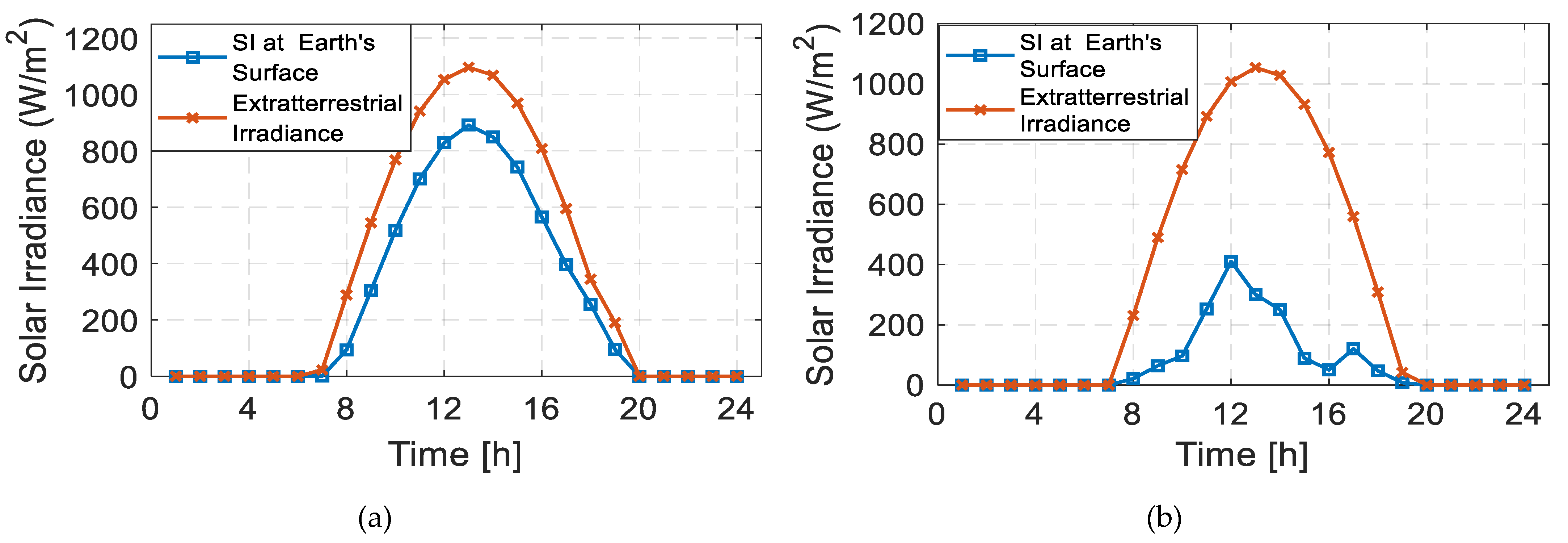
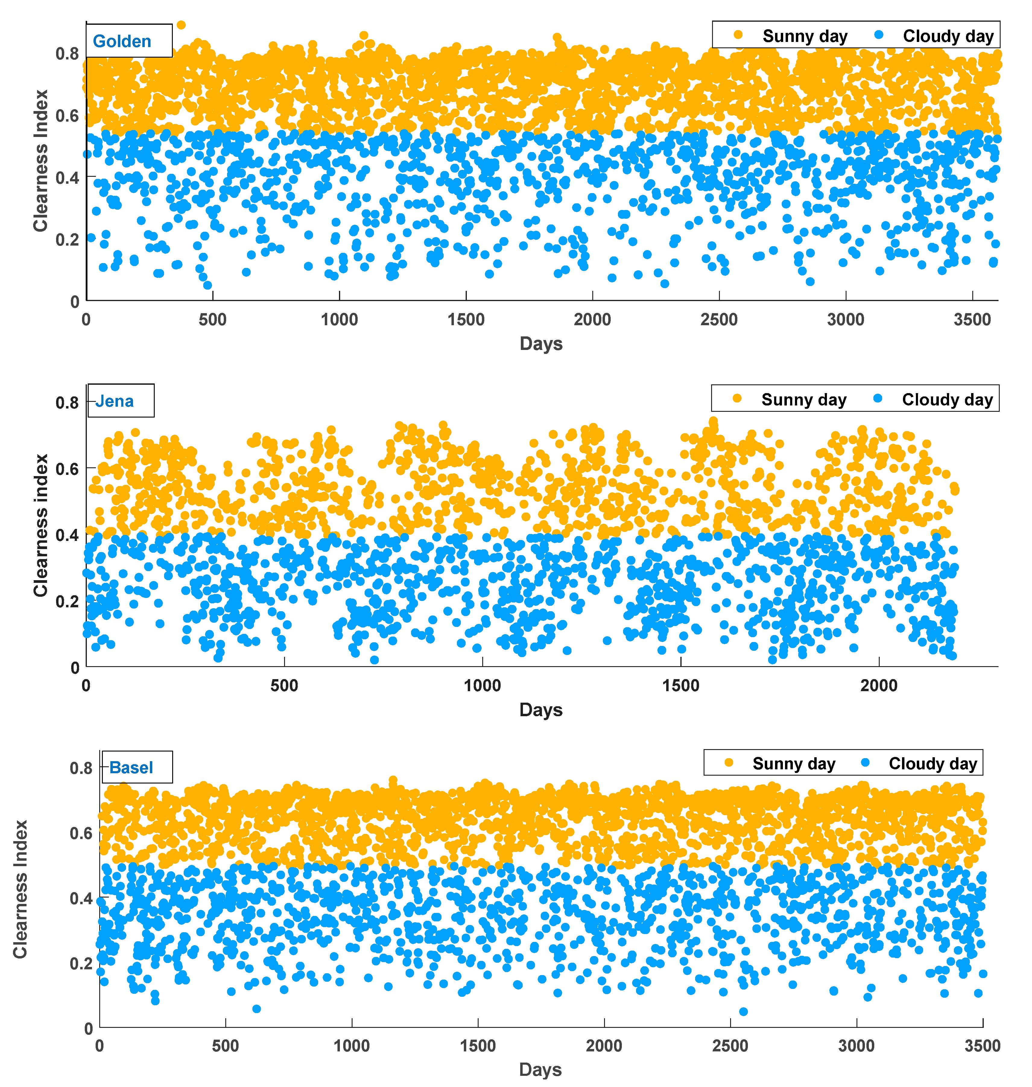
Figure 2 shows the example of sunny and cloudy days, plotted with the corresponding extraterrestrial irradiance.
The proposed hybrid model for SI forecasting consists of the following five steps and the overall flow of the proposed model is shown in
Figure 3.
Step 1: historical data are collected from the weather stations. These data include the SI along with the other weather parameters such as humidity, dew point temperature, etc., that have been previously used as exogenous features in forecasting models.
Step 2: the clearness index for each day is then defined as the ratio of the SI at the surface of the Earth (
I) to the extraterrestrial irradiation (
I0), as shown in Equation (1): [
54]
Thus, the clearness index varies between 0 and 1, where 0 means 100% overcast and 1 indicates clear weather. The values for SI and extraterrestrial irradiation are taken as a daily average to calculate the clearness index. The clearness index can be computed using the SI from weather stations, which is obtained using NWP methods and is available for several days [
55]. In this way, we can classify the next day as a cloudy or sunny day. The accuracy might not be high for such NWP methods. However, these can be used to classify the day as a cloudy or sunny day by averaging the predicted SI for a day.
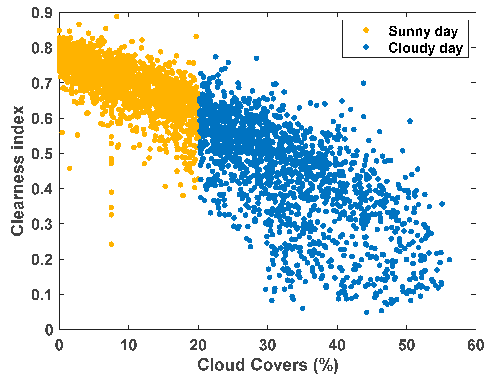
Step 3: k-means clustering is used to divide the data into sunny and cloudy days based on the clearness index. In addition, the classification based on two parameters is also performed to see the effects on accuracy. For this purpose, the percentage of cloud covers with a clearness index is used to classify the day.
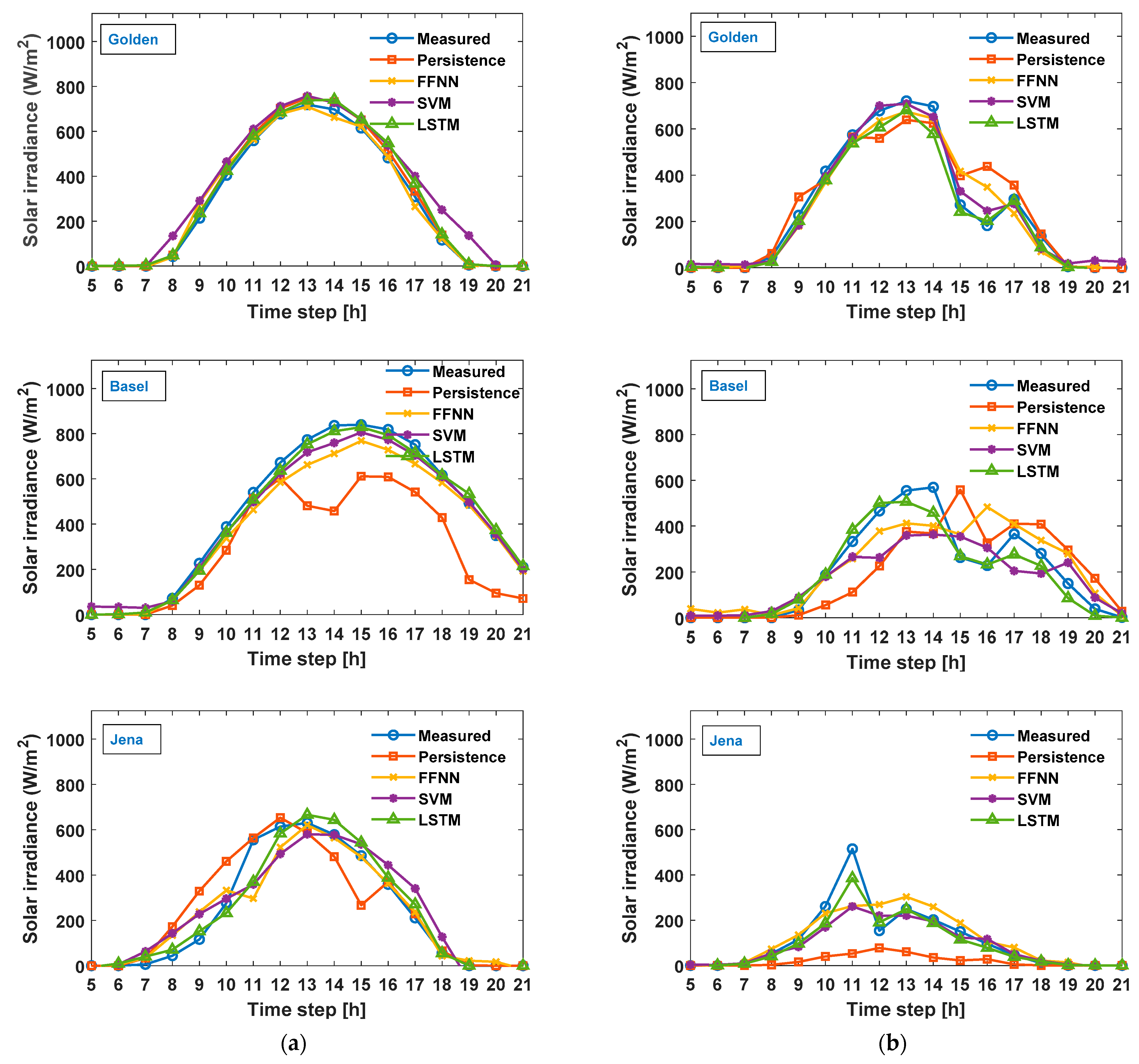
Step 4: the forecasting model is then trained for sunny and cloudy days. For comparison, three models (LSTM, FFNN and SVM) are trained for both days. Each forecasting model is fed with only exogenous features in order to train each model for both types of days.
Step 5: Finally, the results are tested and validated for each type of day via various performance matrices.
As noted in Step 4, although the prime focus of this study is to use the LSTM forecasting model with the clustering approach using exogenous features, the results are compared with those obtained using the other forecasting models (i.e., FFFN and SVM). In addition, the k-means clustering is used with the FFNN and SVM models in order to provide a fair comparison. Each of these models is described and discussed in the following subsections in order to provide a better intuition regarding their mechanisms.
Detailed LSTM-RNN Architecture with k-Means Clustering
The primary focus of the present study is to train the LSTM-RNN network using the results of classification. In this approach, SI data were fed into the k-means clustering algorithm. The clearness index was calculated from the extraterrestrial irradiance and surface solar irradiance via Equation (1). The days were accordingly classified as sunny or cloudy. The results were then used to train the LSTM-RNN network for each day type from the associated data. The detailed architecture of the proposed approach is shown in
Figure 4.
After classification, the LSTM network is trained for each day type. From
Figure 4, dashed boxes represent the training examples that input to the LSTM network. The feature dimensions
for
M number of training examples include exogenous and categorical features for each example, where
t presents the time steps, which are 24 h in day-ahead forecasting for each training example.
The network consists of various layers, including the input layer, several LSTM-based hidden layers, the fully connected layer, and the output layer. The inclusion of more than one LSTM-based layer increases the depth of the network and helps it to learn the temporal dependencies associated with the relevant time steps. The fully connected layer and output layer are used to output the predicted result.
From the input layer, the first-time step of the training example is fed to the first LSTM unit. The initial state of the network is also fed into the LSTM unit in order to compute the first output . It updates cell state as well. At time step t, the corresponding LSTM unit takes the current state of the network () and time step from training example to generate the output and update the cell state . After passing the examples from the network, final outputs for day-ahead SI are generated as .
4. Implementation Details
The experimental description for the proposed methodology is presented in this Section. Separate subsections are dedicated to dataset description, data division, feature selection, and hyperparameter optimization.
4.1. Dataset Description
To demonstrate the diversity of the proposed study, datasets from three locations in the USA, Germany, and Switzerland are included. Information about the sizes of the dataset, latitude and longitude for all locations are mentioned in
Table 1.These datasets were recorded from the following weather stations: The Solar Radiation Research Laboratory (SRRL) in Golden, Colorado (USA) [
56], the weather station at the Max Planck Institute of Biochemistry (MPIB) in Jena (Germany) [
57], and the weather station in Basel, Switzerland [
58].
These datasets include the other parameters to be considered along with SI for the present study, including the dew point temperature, the relative humidity, the dry bulb temperature, cloud covers, wind speed, etc. These are taken as the exogenous features. These obtained input features are the measured values. For the proposed model, these are assumed as the perfectly forecasted values because these exogenous features are used as the forecasted metrological data for the next day as inputs to predict the SI.
4.2. Data Division
In many studies, the datasets are divided into training and testing sets only. In the present study, the datasets are divided into training, validation, and test sets. The distributions of the datasets are detailed in
Table 2. The training set is used to train the proposed model. The validation set is used to tune the hyperparameters, regularization, and feature selection process. Finally, the test set is used to evaluate the performance of the model. Results for validation data sets are reported in
Appendix B. Performance of the proposed model is evaluated and discussed using test sets in
Section 4.
4.3. Feature Selection
Feature selection is crucial to the performance of the forecasting algorithm [
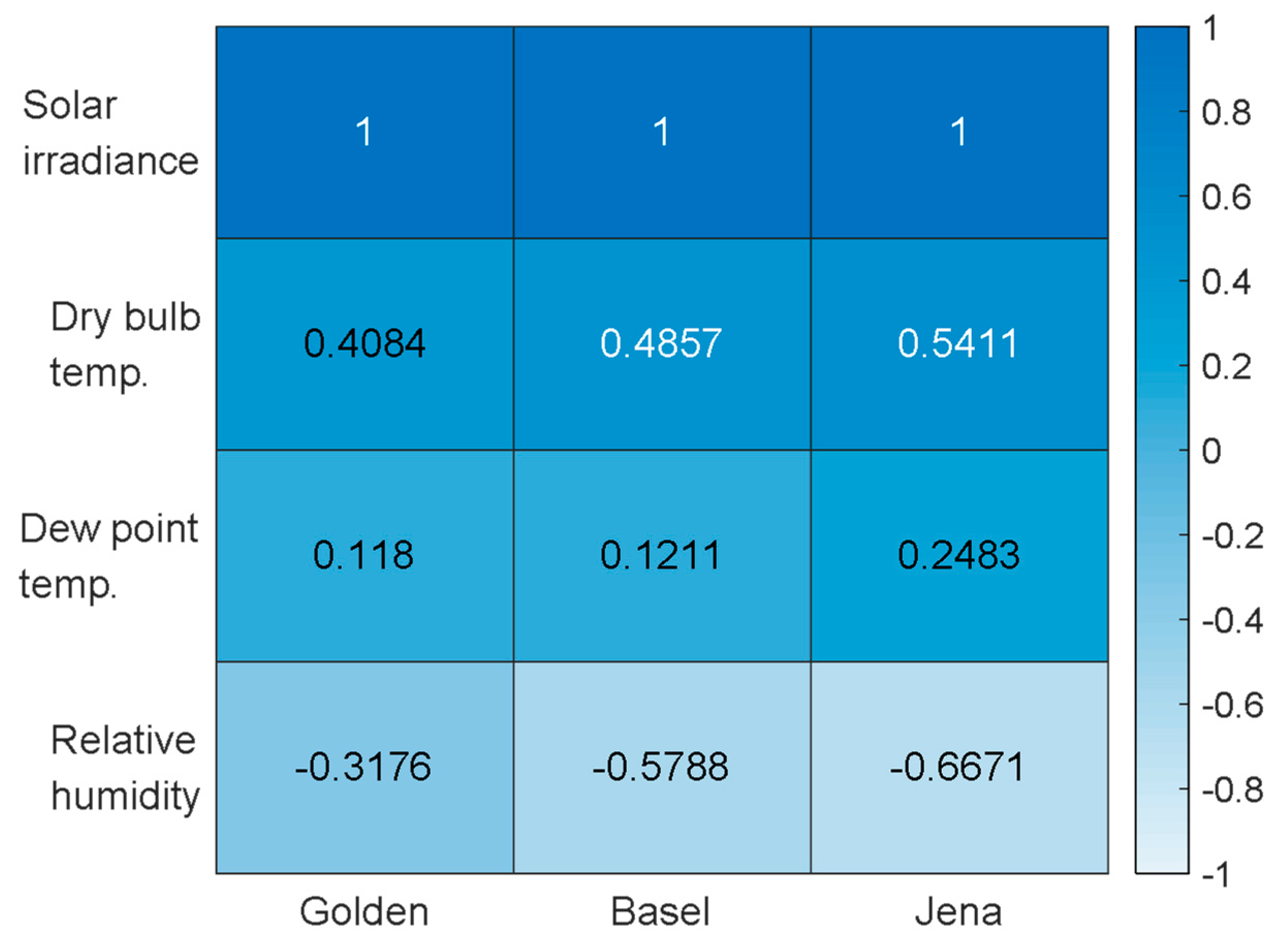
59]. In the present study, the SI was selected for the unsupervised k-means clustering of the datasets in order to classify the days as either sunny or cloudy day. For the LSTM-RNN, model external parameters (exogenous input parameters) are selected to train it for clustered data. The correlation of the external parameters with the SI was calculated using Pearson’s correlation coefficient (PCC). It enables to see the relevancy of the external parameters towards the SI. The PCC ranges from −1 to +1, with a value close to +1 indicating a higher correlation and values approaching −1 indicating a negative or inverse relationship. For example, relative humidity has a negative value that shows an inverse relationship with SI. In this case, if relative humidity goes high, SI goes down and vice versa. PCC of external parameters with SI is shown in
Figure 5. At the x-axis, the locations are mentioned whereas, the y-axis presents the variables including SI and other external parameters. Each box shows the PCC value for the variable with SI.
Provided two variables (
X,
S), the formula for calculating
PCC is given below in Equation (2):
where
μ and
σ are the mean and standard deviation of the variables (
X,
S), and
N is the number of observations in each variable.
For the proposed study, an error evaluation approach was used to select the suitable features among the exogenous features, i.e., listed in
Section 4.1. This approach is known as the wrapper approach [
60]. According to this approach, errors for all the possible variable subsets are evaluated using evaluation metrics such as RMSE, in this study. We evaluated the results for various combinations of the variables (exogenous inputs) and find out the combination that showed the minimum error. The error was evaluated using training and validation sets. The features’ selection method indicated that the dry-bulb temperature, the dew point temperature and the relative humidity were the best choices for the analysis.
For features selection, various other methods are reported that are related to correlation methods. Nevertheless, the wrapper approach is used in this study. Using other correlation methods for feature selection, may not give us good performance because the correlation of a feature can be irrelevant by itself. However, it can provide better performance improvement when combining with other features.
To further highlight the improved performance, additional categorical features are introduced to this methodology, namely: the hours of the day (1–24) and the months of the year (1–12).
4.4. Hyperparameter Tuning
As well as depending on the feature selection process described in
Section 4.3, the performance of the forecasting model is highly dependent on the selection of the hyperparameters that are used for tuning the learning rate. Moreover, the hyperparameter selection also affects the computation and memory factors. Therefore, optimization of the hyperparameters is always a point of debate among researchers. Nevertheless, some rules have been defined by scientists and researchers for setting the values. In the present study, the following hyperparameters were considered for tuning the model: feature scaling, learning rate, optimization solver, number of epochs, dropout rate, number of hidden units, and number of hidden layers.
As the computation significantly depends on the learning rate, this is the most important hyperparameter. For the optimization solver, the adaptive moment estimation (ADAM) [
61], stochastic gradient descent with momentum (SGDM) [
62], and RMSprop [
63,
64] algorithms were tested, and SGDM was found to be the best solver. For hyperparameter optimization, search space is defined based on the trial and error method. Based on the defined search space, the hyperparameters were finally optimized.
Table 3 shows the hyperparameters with the chosen optimal value for the LSTM-RNN model from the search space. In addition, hyperparameters were optimized using only the Golden dataset and applied these same parameters to other datasets. It avoids the over tuning of the model.
The number of hidden layers was optimized as 3 and the hidden units were optimized as 24. Feature scaling showed the best results with a standard scaler method. The dropout rate was set to 0.1, which also works to avoid the overfitting problem. Finally, the number of epochs was tuned to 1500.
By contrast, the hyperparameters used for the FFNN network were the same as in a previous study [
44], i.e., the learning rate was 0.001, the number of hidden units was 10, and 2 hidden layers were set. Full batch gradient descent was used, along with L2 regularization, standard scalar, and 1000 epochs.
For the SVM algorithm, standard feature scaling and a gaussian kernel were used with a sequential minimal optimization (SMO).
4.5. Performance Evaluation
The performance was evaluated using four indicators that are widely used in the literature to evaluate the performance of forecasting models. These are: the root mean square error (RMSE), the normalized root mean square error (NRMSE), the mean absolute error (MAE), and the normalized mean absolute error (NMAE), as defined by Equations (3)–(6) [
65,
66,
67]:
where
and
are the actual and predicted points, and
N is the total number of samples. Thus, normalization of the RMSE and MAE is performed using the min-max method.
6. Conclusions
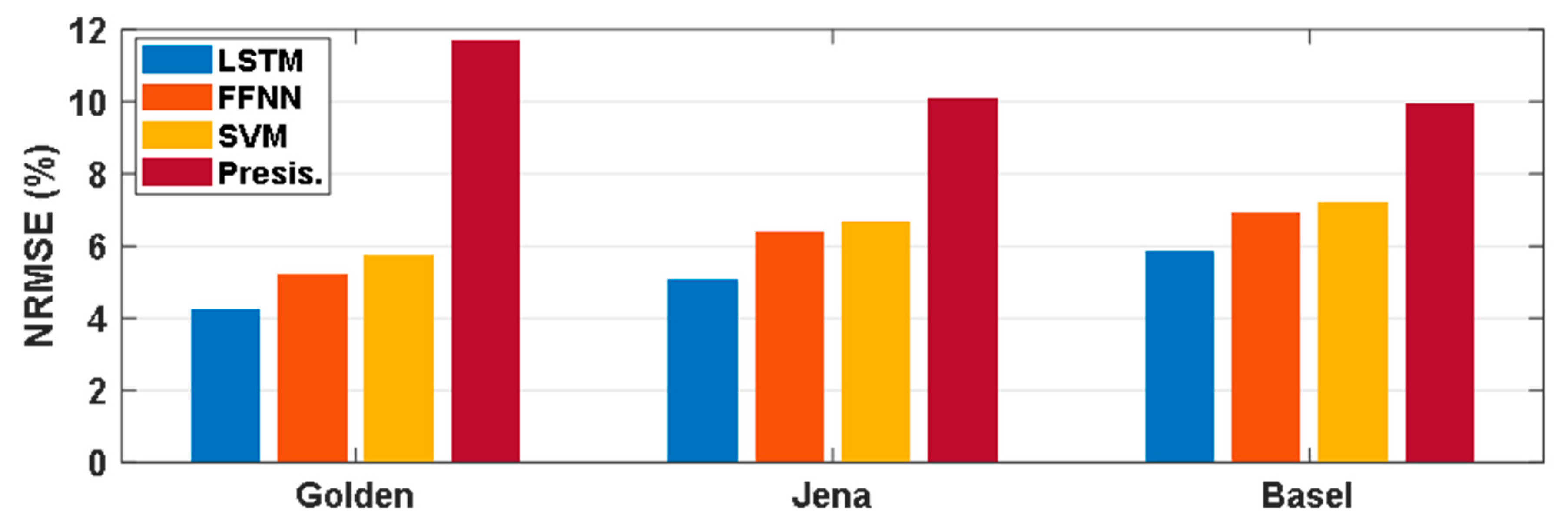
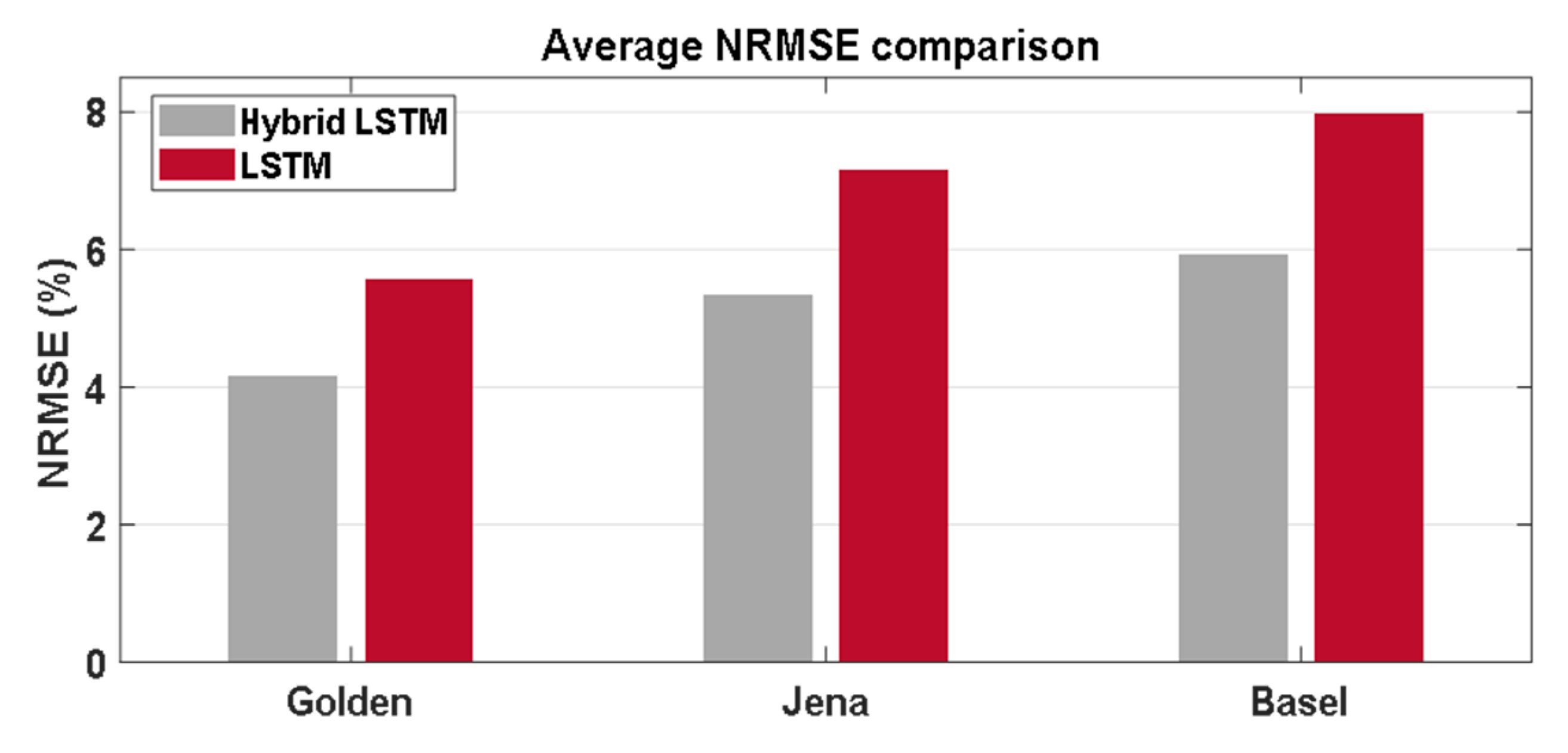
In this paper, a hybrid LSTM-RNN framework for forecasting the SI was proposed and compared with the hybrid approach with FFNN and SVM. K-means clustering was used to classify the days as either sunny or cloudy, then the LSTM-RNN model was used to forecast the SI, and exogenous features were used to train the model. The proposed model was shown to provide the best performance for all three study locations (Golden, Colorado (USA), Jena (Germany), and Basel (Switzerland)) followed by the FFNN and SVM models. In detail, the hybrid LSTM provided maximum and minimum average NRMSEs 4.15% and 5.93% over both types of the day at Golden and Basel, respectively. In terms of the NMAE, the average error percentage was around 2% for both types of day. Overall, the proposed model provided better performance on sunny days than on cloudy days. Furthermore, the hybrid LSTM model exhibited less error than the conventional LSTM model, as indicated by the maximum NRMSEs of 4.15% and 5.56%, respectively.
In addition, the proposed approach is tested for classification considering two parameters (clearness index and cloud covers). Results have shown no improvement in the forecasting as compared to the former way of clustering. Therefore, using one dimension k-means clustering should be significant to use with the advantages of better performance and less computational burden. Finally, it is concluded that as compared to other methods, the proposed hybrid approach to day-ahead SI forecasting can be a more suitable option for power-system applications such as unit commitment, economic dispatch, and other day-ahead market operations.
In future works, we are aiming to perform the analysis and comparison on the effect of errors from forecasted meteorological data. More analysis will be performed on k-means clustering with various combinations of the parameters to see the effect of the classification on the overall model performance. Furthermore, generalization of the proposed model will be performed to make the model more suitable for practical use.


