Abstract
Response surface methodology (RSM) has been widely recognized as an essential estimation tool in many robust design studies investigating the second-order polynomial functional relationship between the responses of interest and their associated input variables. However, there is scope for improvement in the flexibility of estimation models and the accuracy of their results. Although many NN-based estimations and optimization approaches have been reported in the literature, a closed functional form is not readily available. To address this limitation, a maximum-likelihood estimation approach for an NN-based response function estimation (NRFE) is used to obtain the functional forms of the process mean and standard deviation. While the estimation results of most existing NN-based approaches depend primarily on their transfer functions, this approach often requires a screening procedure for various transfer functions. In this study, the proposed NRFE identifies a new screening procedure to obtain the best transfer function in an NN structure using a desirability function family while determining its associated weight parameters. A statistical simulation was performed to evaluate the efficiency of the proposed NRFE method. In this particular simulation, the proposed NRFE method provided significantly better results than conventional RSM. Finally, a numerical example is used for validating the proposed method.
1. Introduction
Among the many quality engineering methodologies, robust design (RD) based on statistical design and analysis methods and optimization methods have contributed significantly to the improvement of product/process quality for more than 20 years. The main objective of RD is to identify the optimal factor settings that can minimize both variability and bias (namely, the deviation between the process mean and desired target value) in a process/product. To demonstrate this RD principle, Taguchi introduced a two-step model based on new design and analysis approaches, particularly orthogonal array and signal-to-noise ratios []. However, orthogonal arrays, statistical analysis, and signal-to-noise ratios are highly controversial [,,,]. Consequently, Vining and Myers [] improved Taguchi’s model by proposing dual-response (DR) estimation and optimization approaches, in which the separate functions of the mean and variance responses are estimated using response surface methodology (RSM) based on the least-squares method (LSM). Their proposed optimization approach can calculate robust factor settings by minimizing process variability while maintaining the process mean at the target value. This results in the primary procedure of RD being identified in three sequential steps: design of experiment (DoE), response function estimation, and optimization. However, Lin and Tu [] pointed out that process bias and variability are not considered simultaneously in the DR model and proposed a mean square error (MSE) model as an alternative approach providing more model flexibility when compared with that provided by the DR approach. These DR and MSE models were further extended by Del Castillo and Montgomery [], Copeland and Nelson [], Cho et al. [], Ames et al. [], Borror [], Kim and Lin [], Koksoy and Doganaksoy [], Ding et al. [], Shin and Cho [,,], Robinson et al. [], Fogliatto [], Goethals and Cho [], Truong and Shin [,], Nha et al. [], Baba et al. [], and Yanıkoğlu et al. [].
In the response function estimation step of the RD procedure, RSM is used extensively to obtain the estimated function associated with an output response and its associated input factors based on the DoE results. RSM is applied extensively in real-world industrial situations, mainly where several input factors potentially affect a product or process’s performance measures or quality characteristics []. The relationship between several input factors and one or more associated output responses can be estimated using RSM. Conventionally, LSM can estimate the unknown coefficients of a regression model with many specific error assumptions, such as the errors in the output responses should be followed by a normal distribution (i.e., zero mean and constant variance) identically and independently. However, these assumptions are often violated in many practical problems. Several alternative approaches, such as transformation, weighted least squares (WLS), maximum-likelihood estimation (MLE), Bayesian, and inverse problems, can be used to address this problem. For example, the WLS method has been applied to RSM to estimate the model parameters for unbalanced data [,], and Lee and Park [] and Cho et al. [] have integrated an MLE method and an expectation–maximization algorithm for unknown parameter estimations using incomplete data. In addition, Goegebeur et al. [] and Chen and Ye [,] proposed a Bayesian approach to estimate the coefficients of response functions where the variances follow a log-normal distribution. Truong and Shin [,] proposed a new estimation method that used an inverse problem approach based on Bayesian perspectives. Most of the existing estimation methods in the RSM and RD literature attempt to generate functional forms in input factors for output responses (namely, the process mean, process variance, and quality characteristic). However, relaxing the error assumptions and increasing the estimation precision would result in further improvements.
Artificial neural networks (ANNs) or neural networks (NNs) with nonlinear mapping structures using the human brain function have been widely used as powerful tools in data classification, forecasting, clustering, function approximation, and optimization in recent decades. Irie and Miyake [], Hornik et al. [], Cybenko [], and Funahashi [] recently addressed the question of approximation using feed-forward NNs and proved that NNs are universal functional approximators with the desired accuracy. ANNs belong to a class of self-adaptive and data-driven techniques, and therefore the undefined relationships between input factors and outputs of a process/product can be ascertained effectively. ANNs can provide a linear or nonlinear relationship between inputs and several outputs without any assumptions based on generalizing capacities of the activation function. Consequently, the functional relationships between input factors and their related output responses in an RD procedure can be estimated without any specific assumptions effectively. Most of the literature on NN function approximation has concentrated on their structure, hidden layers, hidden neurons, and training algorithms. On the contrary, less of them focus on the transfer or activation function, which can strongly affect the complexity and performance of NNs. In addition, most of the transfer functions reported in the literature can provide only a particular configuration to transfer the information from inputs to the associated outputs of a neuron.
The desirability function (DF) approach is one of the most commonly utilized techniques for multiple response optimization problems, in which each quality characteristic is converted into an individual DF that takes a value ranging from 0 to 1. The DF concept was introduced by Harrington [] for the simultaneous optimization of multiple response problems in the industry field. This approach can be used to determine those optimal factors settings of input variables that result in the most desirable output values, while none of these response values are beyond the specified boundaries. Derringer and Suich [] implemented a further extension of Harrington’s DF. Depending on whether the response will minimize, maximize, or specify the desired target value, there are three associated DFs: STB (smaller is better), NTB (nominal is better), and LTB (larger is better). Based on the weight parameters, the DF family may provide a flexible transfer function configuration.
Rowlands et al. [] integrated an NN approach into RD and used the NN to perform the DoE. Su and Hsieh [], Cook et al. [], Chow et al. [], Chang [], and Chang and Chen [] combined an NN approach as an estimation method with a genetic algorithm to determine the optimal process parameter settings or the optimal costs in both static and dynamic characteristics in Taguchi’s formula without considering the process mean and variance functions. Recently, Arungpadang and Kim [] presented a feed-forward NN structure based on RSM in the RD concept.
In the robust design (RD) concept, the process mean and standard deviation of an output response in experiment results can be estimated as a function by many different statistical approaches (i.e., LSM, MLE, and so on). These processes mean and standard deviation functions can be optimized simultaneously based on their desired targets using existing optimization methods. The significant objective of this paper is to propose an alternative estimation method to DR functions (i.e., mean and standard deviation functions) by integrating NN approaches for RSM and RD modeling and then to compare this method to the conventional LSM-based estimation method. First, a feed-forward NN is integrated into the RD procedure as a new DR estimation approach to estimate the process mean and standard deviation response functions. In order to develop the new NN-based estimation method, many different types of transfer functions that can affect the quality of estimation results should be considered.
For this reason, DFs can be utilized as a transfer function family because DFs can represent all three different types (i.e., L-type, S-type, and N-type) of quality characteristics. Among these transfer functions based on DFs, the best transfer function for experimental data using the identified learning and validation approaches is then investigated in this proposed approach. This proposed best transfer function determination procedure for a given NN structure based on DF is derived for the proposed DR estimation method. DFs with their associated weight parameters can provide a variety of transfer function families. In addition, the process mean is often kept at the target value, and the process standard deviation is minimized to the least possible in the RD methodology. Therefore, the “nominal is best” and “smaller is better” DFs are proposed as new NN transfer functions. Next, the best transfer functions for the process mean response function and standard deviation response function are determined based on the optimal weight parameters of the proposed transfer functions using MLE. The associated confidence intervals for the optimal weight parameters are also determined. The results of a case study are presented to support the view that better solutions are obtained from the proposed feed-forward NN-based DR estimation method compared with those from the conventional LSM method and the feed-forward NN estimation approach by using the conventional log-sigmoid transfer function. An overview of the proposed NN-based DR function estimation method is presented in Figure 1.
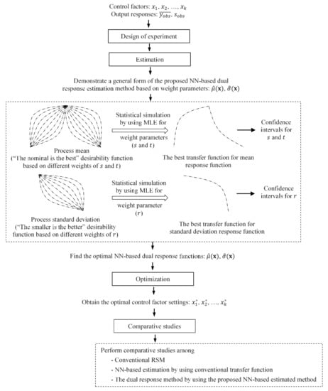
Figure 1.
Overview of the proposed NN-based DR function estimation method.
2. RD Estimation Method Based on RSM
RSM, developed by Box and Wilson [], consists of mathematical and statistical techniques based on the fittings of empirical models obtained from an experimental design. RSM can estimate the functional empirical relationship between the input factors and their related output responses. The basic theory, estimation methods, and analytical techniques of RSM can be found in the study by Myers and Montgomery []. Myers [] and Khuri and Mukhopadhyay [] provide insights into the various developmental stages and future directions of RSM. In general, the output response can be identified as a function of the input factor x as follows:
where x, β, and ε denote the vector of control factors, column vector of model parameters, and random error. The estimated second-order models for the process mean and standard deviation functions are represented as follows:
where and are the estimators of the unknown parameters in the process mean and standard deviation functions, respectively. These coefficients are estimated using the conventional LSM, as follows:
where , , and are the observation average, the standard deviation of replicated responses, and design matrix, respectively.
3. Proposed Feed-Forward NN-Based DR Estimation Method
3.1. Feed-Forward NN Structure
NNs may include a broad class of flexible nonlinear regression, discriminant and data reduction models, and nonlinear dynamical systems []. An NN consists of simple, highly interconnected computational units called artificial neurons. Zainuddin and Pauline [] demonstrated that feed-forward NNs from the input to the output are the most popular NNs for use in function approximation. In addition, Cybenko [], Hornik et al. [], Funahashi [], and Hartman et al. [] demonstrated that a feed-forward NN including one hidden layer could approximate a continuous, arbitrary nonlinear, and multidimensional function. Both processes mean and standard deviation can be two output response characteristics of interest in the RD methodology. The proposed feed-forward NN-based method for estimating the functional relationship associated with input factors and output responses in the RD is depicted in Figure 2.
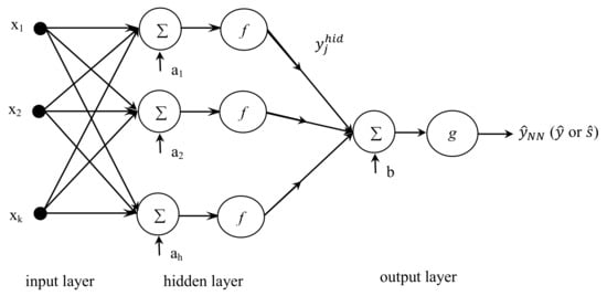
Figure 2.
Proposed feed-forward NN-based RD estimation method.
A vector comprising control factors ,…, , …, , named as the input layer, is the input to the hidden neuron in the hidden layer. The summation of inputs of neurons with identified weights (i.e., coefficients) and bias is transformed using the transfer function to generate the associated output of the hidden neuron. The outputs of the hidden neuron are used as inputs to the neuron in the output layer. Assume that there are h hidden nodes , , ,, and denotes the weight connecting input factor to hidden node the weight connecting hidden node to the final output, the bias at the hidden node , and the bias at the output, respectively. Then, the general form of the response function obtained using the proposed NN-based estimation method is as follows:
3.2. Back-Propagation Learning Algorithm
Among the learning algorithms reported in the literature for performing NN estimation, the back-propagation algorithm is commonly used for training a network owing to its simplicity and applicability []. This algorithm comprises two sequential steps: first, the weights of the NN are initialized randomly, and then, the output of the NN is computed and compared with the actual output. The error at the output layer, that is, the network error, is calculated by comparing the actual output to the desired value to iteratively adjust the weights of the hidden and output layers in accordance with the following function:
Epoch is a hyperparameter that defines the number of times the entire training vectors are used to update the weights. During the training process, the error is optimally minimized. The iterative step of the gradient descent algorithm changes weights based on the following relationship:
The parameter is called the learning rate. There are numerous variations in the basic algorithm based on other optimization techniques (namely, conjugate gradient and Newton methods).
The Marquardt–Levenberg algorithm (trainlm) approximates Newton’s method, which is designed to approach the second-order training speed without applying the Hessian matrix.
The resilient back-propagation training algorithm (trainrp) is a local adaptive learning technique, which performs supervised batch learning in a feed-forward NN. Trainrp removes the negative impact of the dimension of the partial derivative. Therefore, only the sign of the derivative implies the direction of a weight update process.
4. Proposed Transfer Functions Based on DFs
4.1. Integration of DFs into Transfer Functions
DF scales the possible response (y) value to the range of [0, 1], where and represent completely undesirable and desirable values, respectively. Among the three DFs proposed by Derringer and Suich [] for three situations of a particular response, the “nominal is best” and “smaller is better” DFs are utilized as new transfer functions in the hidden NN layers in order to estimate the process mean and standard deviation functions. Assume that there are runs, and hence, the summation at each hidden neuron represents vector consisting of values, where the input of each hidden neuron can then be calculated as at each run order. Therefore, the associated DF output can be represented as . When a response belongs to the “nominal is best” case, the individual DF is defined as
When a response needs to be minimized, the individual DF is
where , , and denote the lower specification, target, and upper specification values, respectively. Superscripts and in Equation (8) and superscript in Equation (9) represent weight parameters of the “nominal is best” and the “smaller is better” DFs, respectively. When the values of and are set to 1, the DFs become linear. For , , and the functions are convex, and for , , and the functions become concave. The integration of the “nominal is best” and “smaller is better” DFs as new transfer functions in the hidden layers to estimate the process mean and standard deviation is depicted in Figure 3.
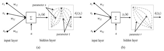
Figure 3.
Integration of DFs as transfer functions in hidden layers: (a) “nominal is best” transfer function and (b) “smaller is better” transfer function.
From Equation (5), the proposed estimated process mean and standard deviation functions (namely, and ) are defined, respectively, as
where , , , , , , , , , , , and denote the number of hidden neurons, bias at the hidden node , bias at the output neuron, weights connecting hidden node to the output responses, weights connecting input factors to hidden node of the proposed feed-forward NN, and the optimal DFs for the process mean and standard deviation functions, respectively. In addition, the log-sigmoid and linear functions are usually used as conventional transfer functions in hidden and output layers, respectively. The conventional log-sigmoid function and linear function with input layer are given as
Similarly, the estimated process mean and standard deviation functions are given, respectively, as follows:
where , , , , , , , , , and denote the number of hidden neurons, bias at hidden node , bias at the output neuron, weight connecting hidden node to the final output, and the weight connecting input factor to hidden node of the feed-forward NNs for the process mean and standard deviation functions, respectively.
4.2. Estimation of Weight Parameters for NN Transfer Functions
The DF can provide a flexible NN transfer function family based on various values of the weight parameter. Among the likelihood-based estimation methods, the MLE method was proposed to estimate the optimal weight parameters for NN transfer functions. On the premise that DF values follow a normal distribution , the distribution of summation can be inferred.
4.2.1. Estimation of Parameter
Using Equation (8), the parametric family in this case can be given as . Based on the principles of MLE, parameters can be identified when log-likelihood functions or are the highest. The log-likelihood function in relation to summation is obtained by multiplying the normal probability density function by the Jacobian of the DF, :
where
Therefore, the log-likelihood function is
For a fixed value , obtaining the derivative of with respect to , setting this derivative function equal to zero, and solving this function by yields
Further, obtaining the derivative of with respect to , assuming it equal to zero, and solving for yields
Accordingly, the log-likelihood function can be represented as follows:
Optimal value is specified using the statistical simulation method.
4.2.2. Estimation of Parameter
Similarly, from Equation (8), the log-likelihood function for parameter is
The profile log-likelihood function used to estimate parameter can be defined as follows:
Optimal value is also identified using the statistical simulation method.
4.2.3. Estimation of Parameter
Using Equation (9), the log-likelihood function for parameter is
The profile log-likelihood function can then be defined as follows:
Optimal value is also determined using the statistical simulation method.
4.3. Confidence Intervals for Weight Parameters
The asymptotic distribution of a maximum likelihood estimator is proposed to identify confidence intervals for weight parameters because the distribution of parameter estimated using MLE is asymptotically normal []. An approximate confidence interval for a parameter can be given as follows:
where refers to the percentile of the standard normal distribution and represents the estimated value of the standard error of . Based on the estimates of the parameters , the standard errors of the parameters can be defined by the square root of the diagonal elements of the estimated covariance matrix. First, the distribution of is stated, followed by the derivation of the approximate asymptotic distribution of parameters , or .
The first derivative of log-likelihood function can be given as
The observed Fisher’s total information matrix is given as
Therefore, Fisher’s total information matrix can then be defined as follows:
The distribution of as converges to a normal distribution. In particular,
where is Fisher’s total information matrix []. is typically not known, but by substituting a consistent estimator, for in Equation (29), the same result can be obtained. Accordingly,
4.3.1. Confidence Intervals for Parameter
The general parameter can be determined as . From Equation (27), can be given as
From the log-likelihood function in Equation (17), can be calculated as follows (see Appendix A.1):
The square root of the diagonal elements of represents an estimate of the standard error for each estimator. An estimator for the standard error of is of particular interest and can be found using the inverses of the partitioned matrices. First, the partition is as follows:
Next, one estimator for can be obtained as follows:
The associated standard error of can be calculated by
Therefore, an approximation confidence interval of can be obtained by using
4.3.2. Confidence Intervals for Parameter
Similarly, a confidence interval of can be obtained by using
The standard error of can be defined as follows (see Appendix A.2):
4.3.3. Confidence Intervals for Parameter
Similarly, an confidence interval of can be obtained by using
The standard error of can be defined as follows (see Appendix A.3):
5. Case Study
This case study was performed using the printing data example proposed by Vining and Myers [] and Lin and Tu []. The impacts of three input factors, that is, speed (), pressure (), and distance (), on the capabilities of a printing machine that applies colored inks to package levels (y) were investigated. Each input factor had three levels, resulting in a total of 27 runs. Three replications were performed for each data combination.
In comparative studies between methods, the expected quality loss (EQL) is usually applied as a critical optimization criterion in RD. The expectation of the loss function is defined as
where represents a positive loss coefficient. , , and are the estimated process mean function, desirable target value, and estimated standard deviation function, respectively. In this case study, the target value was . Using MATLAB, the process-estimated mean and standard deviation functions obtained using the LSM based on RSM were as follows:
where
For comparison, the criteria used in the NN (mainly, the number of hidden neurons, training algorithms, and the number of epochs of NNs) for the conventional log-sigmoid transfer function in the hidden layer were the same as those of the proposed NNs. The NN information for the conventional log-sigmoid transfer function and the proposed DR estimation method are presented in Table 1. The NN architecture consists of several input factors, hidden neurons, and output responses. The weight and bias matrix values of the NNs using the conventional log-sigmoid transfer function for the process mean and standard deviation functions are presented in Table 2. Based on the structures, training algorithms, transfer functions, and the number of epochs of the proposed feed-forward NNs used to estimate the functions of process mean and standard deviation, optimal weight parameters , , and were calculated using Equations (20), (22), and (24), respectively. As shown in Table 3, twenty hidden neurons in the hidden layer are used to estimate mean function, and twenty hidden neurons in the hidden layer are used to estimate standard deviation function. For each hidden neuron, a desirability function is proposed as a transfer function. In addition, weight parameters (i.e., s, t, and r) for DFs identified in Equations (8) and (9) and associated confidence intervals are demonstrated in Table 3. The respective 95% confidence intervals for these weight parameters calculated by using Equations (35), (38), and (40) are presented in Table 3. The weight and bias matrix values of the feed-forward NNs using the proposed transfer functions for the process mean and standard deviation functions are presented in Table 4.

Table 1.
Feed-forward NNs information used to estimate DR functions.
Table 2.
Weight and bias values from the NNs approach by using the conventional log-sigmoid transfer function.
Table 3.
Estimated weight parameters and associated confidence intervals.
Table 4.
Weight and bias values by using the NN-based DR estimation method.
The estimated process mean and standard deviation functions obtained by applying the conventional LSM-RSM, the NN-based estimation method using the conventional log-sigmoid transfer function, and the proposed DR approach with the estimated optimal weight parameters listed in Table 3, along with the associated coefficients of determination of each estimated response function, are illustrated in Figure 4, Figure 5 and Figure 6 as contour plots, respectively.
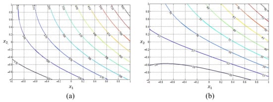
Figure 4.
Estimated process mean and standard deviation response functions from the conventional LSM approach based on RSM: (a) mean (); (b) standard deviation ().
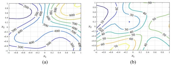
Figure 5.
Estimated process mean and standard deviation response functions from the feed-forward NN approach with conventional log-sigmoid transfer function: (a) mean (); (b) standard deviation ().
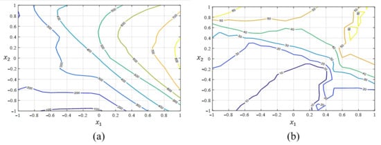
Figure 6.
Estimated process mean and standard deviation response functions from the feed-forward NN approach with the proposed transfer functions: (a) mean (); (b) standard deviation ().
The optimal control factor settings, the optimal process parameters (i.e., process mean, bias, and variance), and their associated EQL values obtained by the three different approaches (i.e., the conventional LSM based on RSM, the NN-based estimation method using the conventional log-sigmoid transfer functions, and the proposed NN-based DR estimation method) are presented in Table 5.
Table 5.
Comparative results of various methods.
As demonstrated in Table 5, the process variance obtained from the NN-based estimation methods is remarkably smaller than that of the conventional statistical LSM approach. Therefore, NN-based estimation methods can provide considerably smaller EQL values (i.e., significant criteria to evaluate the level of quality) than those of the conventional LSM approach in this particular example, although the same RD optimization model is utilized. Of the two NN-based estimation methods, the proposed DR approach provides better optimal solutions when compared with that of the NN-based estimation method that uses the conventional log-sigmoid transfer function because the variance obtained from the proposed DR approach is almost zero in this particular example. Therefore, in terms of EQL, the best optimal solutions can be obtained using the NN-based DR estimation method. The criterion spaces (squared bias vs. variance) of the three estimated functions by using the conventional LSM approach based on RSM, the N-based estimation method using the log-sigmoid transfer function, and the proposed DR approach are illustrated in Figure 7. A green cross marks the optimal settings in each figure.
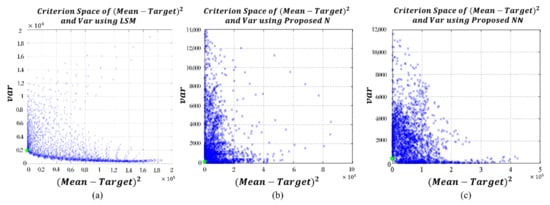
Figure 7.
Criterion spaces of the three estimated functions: (a) LSM based on RSM; (b) log-sigmoid transfer function-based NN; (c) proposed NN-based DR method.
6. Conclusions and Further Studies
This study proposes a feed-forward NN-based DR estimation method to estimate the process mean and standard deviation functions for RSM and RD modeling. The proposed method can avoid basic error assumptions of the conventional LSM approach in this particular situation. Further, integrating the DFs into the NN structures in the proposed method results in a general and flexible transfer function family for transforming data based on the proposed DFs. The optimal weight parameters of the DF family can be determined using the MLE and the confidence intervals of the optimal weight parameters using the proposed asymptotic distribution of maximum-likelihood estimators. The best transfer function in the NN structure was achieved using the proposed method. The proposed NN-based DR estimation method provides better solutions for EQL than those of the conventional LSM approach and the NN-based estimation method that uses the conventional log-sigmoid transfer function in the particular case study example. In order to improve the reliability of the proposed methods, different types of experimental data (i.e., small and large data sets, different DoE results, and small and large sets of replications) should be considered.
In further studies, the assumption that the error follows a normal distribution and whether the DF values can follow any distribution will be investigated. Additionally, the optimal weight parameters of the DF-based transfer functions were estimated using a Bayesian approach or the Newton–Raphson algorithm. We then plan to determine the confidence intervals of the optimal weight parameters using a t-distribution. In addition, a more comprehensive comparative study between the proposed NN models and higher-order models of conventional RSM can be a significant further research issue. Based on this comparative study and a Bayesian approach, we may develop a new optimal estimation system by integrating the proposed NN models and conventional RSM models.
Author Contributions
Conceptualization, T.-H.L. and S.S.; Methodology, T.-H.L. and S.S.; Modeling, T.-H.L.; Validation T.-H.L. and S.S.; Writing—original draft preparation, T.-H.L. and S.S.; Writing—Review and Editing, H.J. and S.S.; Funding Acquisition, H.J. and S.S. All authors have read and agreed to the published version of the manuscript.
Funding
This work was supported by the National Research Foundation of Korea (NRF) (No. NRF-2019R1F1A1060067 and No. NRF-2019R1G1A1010335).
Conflicts of Interest
The authors declare no conflict of interest.
Appendix A. Confidence Intervals for Weight Parameters
Appendix A.1. Parameter s
Fisher’s total information matrix for the general parameter is defined as follows:
The first derivatives of the log-likelihood function for the mean, variance, and parameter can be expressed as follows:
The second derivatives of the log-likelihood function for the mean, variance, and parameter with mixed partials are given as follows:
Consequently, Fisher’s total information matrix can be expressed as
Appendix A.2. Parameter t
General parameter can be determined as . Based on Equation (27), can be expressed as
Based on the log-likelihood function in Equation (21), the first derivatives of the log-likelihood function for the mean, variance, and parameter can be expressed as follows:
The second derivatives of log-likelihood function for the mean, variance, and parameter with mixed partials are given as follows:
Therefore,
The square root of the diagonal elements of represents the standard error for each estimator. An estimator for the standard error of is of particular interest and can be obtained using the inverses of the partitioned matrices. First, the partition is
Next, one estimator for can be obtained as follows:
The associated standard error of can be defined as
Appendix A.3. Parameter r
To estimate parameter, general parameter can be determined as .
From Equation (27),
Based on the log-likelihood function in Equation (23), the first derivatives of the log-likelihood function for the mean, variance, and parameter can be expressed as follows:
The second derivatives of log-likelihood function for the mean, variance, and parameter with mixed partials are given as follows:
Therefore,
The squared root of the diagonal entries of represents the standard error for each estimator. An estimator for the standard error of is of particular interest and can be obtained using the inverses of the partitioned matrices. First, partition is
Next, one estimator for can be obtained as follows:
Finally, the associated standard error of can be defined as
References
- Taguchi, G. Introduction to Quality Engineering; UNIPUB/Kraus International: White Plains, NY, USA, 1986. [Google Scholar]
- Leon, R.V.; Shoemaker, A.C.; Kackar, R.N. Performance measures independent of adjustment: An explanation and extension of Taguchi signal-to-noise ratio. Technometrics 1987, 29, 253–285. [Google Scholar] [CrossRef]
- Box, G.E.P. Signal-to-noise ratios, performance criteria, and transformations. Technometrics 1988, 30, 1–17. [Google Scholar] [CrossRef]
- Box, G.; Bisgaard, S.; Fung, C. An explanation and critique of Taguchi’s contribution to quality engineering. Qual. Reliab. Eng. Int. 1988, 4, 123–131. [Google Scholar] [CrossRef]
- Nair, V.N. Taguchi’s parameter design: A panel discussion. Technometrics 1992, 34, 127–161. [Google Scholar] [CrossRef]
- Vining, G.G.; Myers, R.H. Combining Taguchi and response surface philosophies: A dual response approach. J. Qual. Technol. 1990, 22, 38–45. [Google Scholar] [CrossRef]
- Lin, D.K.J.; Tu, W. Dual response surface optimization. J. Qual. Technol. 1995, 27, 34–39. [Google Scholar] [CrossRef]
- Del Castillo, E.; Montgomery, D.C. A nonlinear programming solution to the dual response problem. J. Qual. Technol. 1993, 25, 199–204. [Google Scholar] [CrossRef]
- Copeland, K.A.F.; Nelson, P.R. Dual response optimization via direct function minimization. J. Qual. Technol. 1996, 28, 331–336. [Google Scholar] [CrossRef]
- Cho, B.R.; Philips, M.D.; Kapur, K.C. Quality improvement by RSM modeling for robust design. In Proceedings of the 5th Industrial Engineering Research Conference, Minneapolis, MN, USA, 18–20 May 1996; pp. 650–655. [Google Scholar]
- Ames, A.E.; Mattucci, N.; Macdonald, S.; Szonyi, G.; Hawkins, D.M. Quality loss functions for optimization across multiple response surfaces. J. Qual. Technol. 1997, 29, 339–346. [Google Scholar] [CrossRef]
- Borror, C.M. Mean and variance modeling with qualitative responses: A case study. Qual. Eng. 1998, 11, 141–148. [Google Scholar] [CrossRef]
- Kim, K.J.; Lin, D.K.J. Dual response surface optimization: A fuzzy modeling approach. J. Qual. Technol. 1998, 30, 1–10. [Google Scholar] [CrossRef]
- Koksoy, O.; Doganaksoy, N. Joint optimization of mean and standard deviation using response surface methods. J. Qual. Technol. 2003, 35, 239–252. [Google Scholar] [CrossRef]
- Ding, R.; Lin, D.K.J.; Wei, D. Dual response surface optimization: A weighted MSE approach. Qual. Eng. 2004, 16, 377–385. [Google Scholar] [CrossRef]
- Shin, S.; Cho, B.R. Bias-specified robust design optimization and an analytical solutions. Comput. Ind. Eng. 2005, 48, 129–148. [Google Scholar] [CrossRef]
- Shin, S.; Cho, B.R. Robust design models for customer specified bounds on process parameters. J. Syst. Sci. Syst. Eng. 2006, 15, 2–18. [Google Scholar] [CrossRef]
- Shin, S.; Cho, B.R. Studies on a bi-objective robust design optimization problem. IIE Trans. 2009, 41, 957–968. [Google Scholar] [CrossRef]
- Robinson, T.J.; Wulff, S.S.; Montgomery, D.S.; Khuri, A.I. Robust parameter design using generalized linear mixed models. J. Qual. Technol. 2006, 38, 65–75. [Google Scholar] [CrossRef]
- Fogliatto, S.F. Multiresponse optimization of products with functional quality characteristics. Qual. Reliab. Eng. Int. 2008, 24, 927–939. [Google Scholar] [CrossRef]
- Goethals, P.L.; Cho, B.R. The development of a robust design methodology for time-oriented dynamic quality characteristics with a target profile. Qual. Reliab. Eng. Int. 2010, 27, 403–414. [Google Scholar] [CrossRef]
- Truong, N.K.V.; Shin, S. Development of a new robust design method based on Bayesian perspectives. Int. J. Qual. Eng. Technol. 2012, 3, 50–78. [Google Scholar] [CrossRef]
- Truong, N.K.V.; Shin, S. A new robust design method from an inverse-problem perspective. Int. J. Qual. Eng. Technol. 2013, 3, 243–271. [Google Scholar] [CrossRef]
- Nha, V.T.; Shin, S.; Jeong, S.H. Lexicographical dynamic goal programming approach to a robust design optimization within the pharmaceutical environment. Eur. J. Oper. Res. 2013, 229, 505–517. [Google Scholar] [CrossRef]
- Baba, I.; Midi, H.; Rana, S.; Ibragimov, G. An alternative approach of dual response surface optimization based on penalty function method. Math. Probl. Eng. 2015, 2015, 450131. [Google Scholar] [CrossRef]
- Yanıkoğlu, İ.; den Hertog, D.; Kleijnen, J.P. Robust dual-response optimization. IIE Trans. 2016, 48, 298–312. [Google Scholar] [CrossRef]
- Myers, R.H.; Montgomery, D.C. Response Surface Methodology: Process and Product Optimization using Designed Experiments, 1st ed.; John Wiley & Sons: New York, NY, USA, 1995. [Google Scholar]
- Luner, J.J. Achieving continuous improvement with the dual response approach: A demonstration of the Roman catapult. Qual. Eng. 1994, 6, 691–705. [Google Scholar] [CrossRef]
- Cho, B.R.; Park, C.S. Robust design modeling and optimization with unbalanced data. Comput. Ind. Eng. 2005, 48, 173–180. [Google Scholar] [CrossRef]
- Lee, S.B.; Park, C.S. Development of robust design optimization using incomplete data. Comput. Ind. Eng. 2006, 50, 345–356. [Google Scholar] [CrossRef]
- Cho, B.R.; Choi, Y.; Shin, S. Development of censored data-based robust design for pharmaceutical quality by design. Int. J. Adv. Manuf. Technol. 2010, 49, 839–851. [Google Scholar] [CrossRef]
- Goegebeur, Y.; Goos, P.; Vandebroek, M. A hierarchical Bayesian approach to robust parameter design. SSRN 2007, 1–23. [Google Scholar] [CrossRef][Green Version]
- Chen, Y.; Ye, K. Bayesian hierarchical modeling on dual response surfaces in partially replicated designs. Qual. Technol. Quant. Manag. 2009, 6, 371–389. [Google Scholar] [CrossRef]
- Chen, Y.; Ye, K. A Bayesian hierarchical approach to dual response surface modeling. J. Appl. Stat. 2011, 38, 1963–1975. [Google Scholar] [CrossRef]
- Irie, B.; Miyake, S. Capabilities of three-layered perceptrons. In Proceedings of the International Conference Neural Networks, San Diego, CA, USA, 24–27 July 1988; pp. 641–648. [Google Scholar]
- Hornik, K.; Stinchcombe, M.; White, H. Multilayer feedforward networks are universal approximators. Neural Netw. 1989, 2, 359–366. [Google Scholar] [CrossRef]
- Cybenko, G. Approximation by superpositions of a sigmoidal function. Math. Control Signals Syst. 1989, 2, 303–314. [Google Scholar] [CrossRef]
- Funahashi, K. On the approximate realization of continuous mappings by neural networks. Neural Netw. 1989, 2, 183–192. [Google Scholar] [CrossRef]
- Harrington, E.C. The desirability function. Ind. Qual. Control. 1965, 21, 494–498. [Google Scholar]
- Derringer, G.; Suich, R. Simultaneous optimization of several response variables. J. Qual. Technol. 1980, 12, 214–219. [Google Scholar] [CrossRef]
- Rowlands, H.; Packianather, M.S.; Oztemel, E. Using artificial neural networks for experimental design in off-line quality. J. Syst. Eng. 1996, 6, 46–59. [Google Scholar]
- Su, C.T.; Hsieh, K.L. Applying neural network approach to achieve robust design for dynamic quality characteristics. Int. J. Qual. Reliab. Manag. 1998, 15, 509–519. [Google Scholar] [CrossRef]
- Cook, D.F.; Ragsdale, C.T.; Major, R.L. Combining a neural network with a genetic algorithm for process parameter optimization. Eng. Appl. Artif. Intell. 2000, 13, 391–396. [Google Scholar] [CrossRef]
- Chow, T.T.; Zhang, G.Q.; Lin, Z.; Song, C.L. Global optimization of absorption chiller system by genetic algorithm and neural network. Energy Build. 2002, 34, 103–109. [Google Scholar] [CrossRef]
- Chang, H.H. Applications of neural networks and genetic algorithms to Taguchi’s robust design. Int. J. Electron. Commer. 2005, 3, 90–96. [Google Scholar]
- Chang, H.H.; Chen, Y.K. Neuro-genetic approach to optimize parameter design of dynamic multiresponse experiments. Appl. Soft. Comput. 2011, 11, 436–442. [Google Scholar] [CrossRef]
- Arungpadang, R.T.; Kim, J.Y. Robust parameter design based on back propagation neural network. Korean Manag. Sci. Rev. 2012, 29, 81–89. [Google Scholar] [CrossRef]
- Box, G.E.P.; Wilson, K.B. On the experimental attainment of optimum conditions (with discussion). J. R. Stat. Soc. B 1951, 13, 270–310. [Google Scholar]
- Myers, R.H. Response surface methodology—Current status and future directions. J. Qual. Technol. 1999, 31, 54–57. [Google Scholar] [CrossRef]
- Khuri, A.I.; Mukhopadhyay, S. Response surface methodology. Wiley Interdiscip. Rev. Comput Stat. 2010, 2, 128–149. [Google Scholar] [CrossRef]
- Sarle, W.S. Neural networks and statistical models. In Proceeding of the 19th Annual SAS User Group International Conference, Dallas, TX, USA, 10–13 April 1994; pp. 1–13. [Google Scholar]
- Zainuddin, Z.; Pauline, O. Function approximation using artificial neural networks. WSEAS Trans. Math. 2008, 7, 333–338. [Google Scholar]
- Hartman, E.J.; Keeler, J.D.; Kowalski, J.M. Layered neural networks with Gaussian hidden units as universal approximations. Neural Comput 1990, 2, 210–215. [Google Scholar] [CrossRef]
- Zilouchian, A.; Jamshidi, M. Intelligent Control. Systems Using Soft Computing Methodologies; CRC Press: Boca Raton, FL, USA, 2000. [Google Scholar]
- Lindsey, J.K. Parametric Statistical Inference; Oxford University Press: New York, NY, USA, 1996. [Google Scholar]
Publisher’s Note: MDPI stays neutral with regard to jurisdictional claims in published maps and institutional affiliations. |
© 2021 by the authors. Licensee MDPI, Basel, Switzerland. This article is an open access article distributed under the terms and conditions of the Creative Commons Attribution (CC BY) license (https://creativecommons.org/licenses/by/4.0/).