1. Introduction
Knee arthroscopy is a minimally invasive surgery (MIS) which is typically performed to diagnose and treat knee joint pathologies. It requires making several small incisions in the knee to allow for the insertion of a surgical tool and an arthroscope, which is an endoscope that provides the surgeon with a 2D view of the surgical site. Based on only the arthroscope view, the surgeon performs the surgical procedure. Despite knee arthroscopy being a common procedure (four million knee arthroscopies performed worldwide annually, at a total cost of US
$15 billion [
1]), it is complex to perform [
1] and can lead to several post-surgical complications, such as unintentional femoral cartilage damage or excessive bleeding [
2,
3,
4]. In a recent study, orthopedic surgeons reported having difficulties visualizing some sections of the knee while operating and that a real-time 3D model of the knee structures would be beneficial [
1]. Real-time (high-refresh-rate) 3D ultrasound (US) can provide the intra-operative volumetric information to obtain this type of model of the surgical site [
5] and can be used in a robotic system to assist in knee arthroscopy [
6]. For these types of applications, it is necessary to automate the interpretation of the 3D US volumes.
This work focuses on automatic arthroscope localization on 3D US volumes. The ultimate goal is to use this information on the position and orientation of the arthroscope to automatically register the 2D camera view with the 3D US volumes. In this way, 3D US will complement the 2D camera image of the arthroscope, as it can provide depth perception and visibility on structures that are not visible on the latter. The combination of the two imaging modalities has the potential to allow for enhanced navigation during surgery, leading to improved surgical outcomes.
In literature, there has been increasing interest in detecting various kinds of medical instruments, such as surgical tools, needles, and catheters on US images. Several methods aim at detecting medical instruments based on their shape and intensity on a specific imaging modality. Methods make, for example, use of projections (reducing a 3D volume to a 2D image based on intensity along the projection axis) in combination with 2D Hough transforms [
7,
8], and Parallel Integration Projections (PIP) [
9]. These methods perform poorly when the medical instrument is shielded by other highly echogenic intensity structures in the path of the projection. Alternative methods are 3D Hough transforms [
9,
10,
11] and Gabor transforms [
12]. However, these methods cannot detect the medical instrument properly if it is not on the plane in which the transformation is applied.
Also, a Frangi’s vesselness measure was used as a line filtering method [
13] to detect surgical tools [
14]. In addition, a combination of the Gabor transform and Frangi’s vesselness measure has been used to create features for a voxel classification algorithm with the goal of medical instrument localization [
15]. These methods overcome some of the shortcomings of the above-mentioned methods. Nevertheless, they still suffer from being dependent on assumptions about the shape and appearance of the medical instrument. This leads to problems when attempting to detect a surgical tool that is partly inserted in tissue or that is surrounded by highly echogenic tissue in the US image, such as the boundaries of bones.
More recently, there has been interest in utilizing supervised deep learning approaches for the detection and segmentation of medical instruments [
16,
17,
18,
19,
20] in 3D US volumes. These approaches show a superior localization performance compared to the more traditional image processing techniques presented in the last paragraph. Furthermore, these approaches can detect partly inserted instruments with different shapes and can perform well in low resolution US volumes. The major drawback of these methods is that they require labels for each voxel in the 3D US volume, which are classified as either a medical instrument or not; or, labels for the medical instrument tip position and axis [
21,
22]. Generating these types of annotations requires significant time and effort from medical professionals. In addition, these annotations may suffer from significant intra- and inter-operator variability [
23,
24], as it is challenging to determine where the boundaries of a structure are exactly located on US images.
To overcome the problem of requiring annotated US volumes, a novel approach for the localization of arthroscopes on 3D US volumes using weakly supervised deep learning [
25] is proposed in this work. This approach only requires assigning an image-level label to each 2D image of the US volume, indicating if the arthroscope is present in the image or not. Therefore, the labelling effort is greatly reduced. Weakly supervised deep learning approaches have been used before to detect anatomical structures on US images of the placenta [
26,
27], breast [
28,
29], lung [
30,
31] and the brain [
32,
33]. These approaches use a combination of (strongly) supervised and weakly supervised methods. For the works which used a completely weakly supervised localization method [
25], the resulting localization is presented as a by-product of the detection and are not interpreted or utilized further.
In this proof-of-concept work, a convolutional neural network based on DenseNet [
34], of which the 2D class activation maps (CAMs) [
35] are used to create 3D bounding boxes [
36], was implemented in order to provide localization information. The main contributions of this work are the interpretation of these CAMs and providing weakly-supervised localization information in 3D instead of in 2D. To the best of our knowledge, no work has been published before on weakly supervised localization of medical instruments on 3D US volumes.
The US volumes used in this study were acquired on a phantom mimicking the imaging conditions of knee arthroscopy and on a human cadaver knee. The localization accuracy results have been visually evaluated and compared with a ground truth position that approximated the position of the arthroscope tip.
2. Materials and Methods
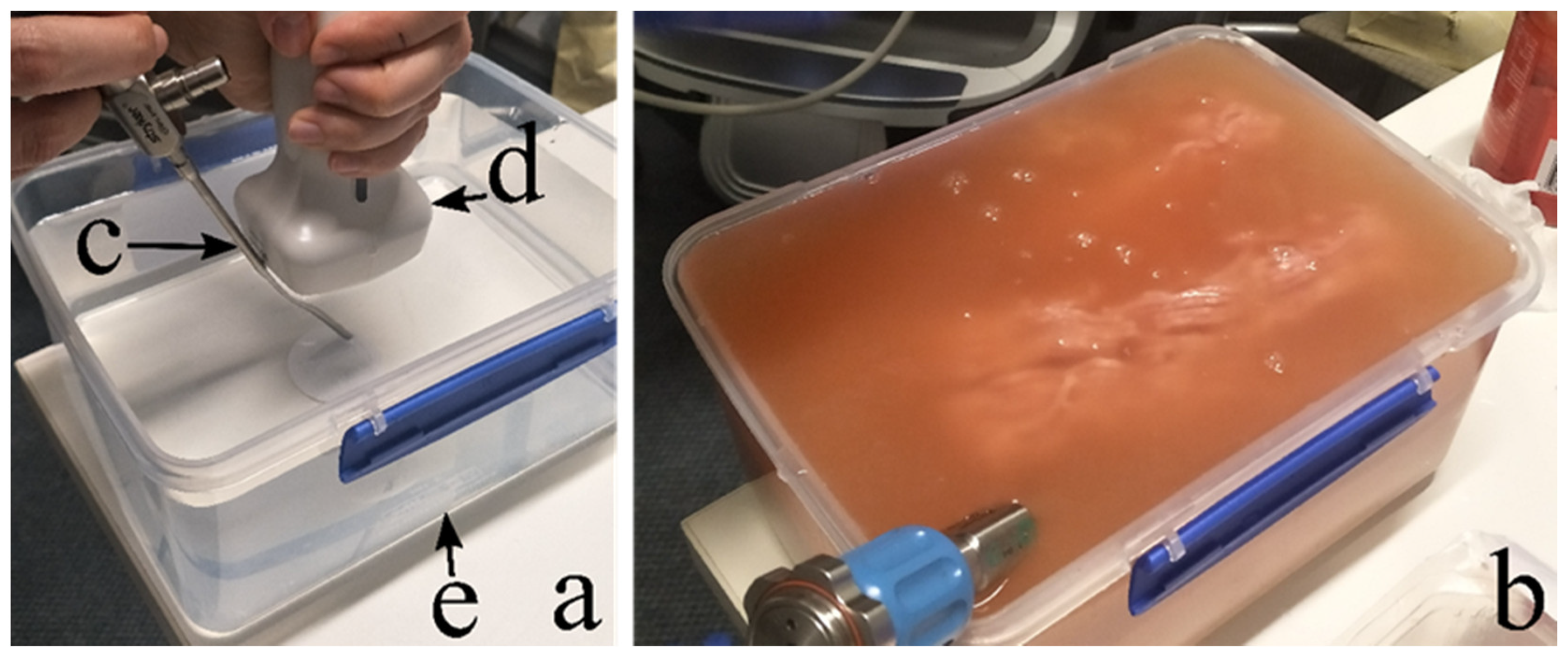
Eighty-one 3D US volumes were acquired using a VL13-5 linear array volumetric probe (Philips Healthcare, Bothell, WA, USA) and an EpiQ7 US system (Philips Medical Systems, Andover, MA, USA). The volumes were acquired on a phantom mimicking the sonographic appearance of human tissue layers with an arthroscope inserted. To this end, water, flour, minced meat, mozzarella cheese and tomatoes were combined in varying quantities inside a plastic container (see
Figure 1). The materials used in this work are similar to materials that have been used for other phantoms, such as pea pods [
37], grapes [
38], tofu and paneer [
39]. Minced meat has been used to mimic (human) tissue as it has a similar appearance, and it is easy to obtain compared to ex-vivo animal samples. Mozzarella and tomato [
40] were added to create hyperechoic structures which can resemble other tissues like bone and muscle. Instead of using the more conventional gelatin, water with flour was used to ensure the appearance of US speckle patterns. The main advantage of using water with flour instead of gelatin is that this results in a dynamic phantom, which can change shape depending on how the arthroscope is inserted. This behavior is similar to a real a knee arthroscopy where the knee is filled with a saline solution and the tissues inside the knee can move under influence of the arthroscope. Furthermore, no traces, which could confuse the deep learning algorithm, are left in the phantom after removal of the arthroscope as is the case for gelatin. Other advantages of this phantom setup are that many different configurations of the structures can be created and, above all, that the complexity of the phantom can be increased from a simple single homogeneous component to a complex combination of materials with different echogenic characteristics. This was very helpful to guide the development of the algorithms in a progressive way.
Table 1 details the different phantom types, material compositions, the number of US volumes and the corresponding number of 2D US images for each type. Phantom type 0 through 5 were used to create a training, validation and test set. (See below for more details). Phantom type 6 through 8 were used for performance evaluation of the network only (see below for more details). The acquired US volumes have varying image properties due to:
The composition and location of the phantom ingredients.
Changes in the insertion angle and penetration depth of the arthroscope.
Changes in the location and angle of the US probe with respect to the acoustic window of the phantom.
Changes in the US volume dimensions and voxel sizes.
In addition, one US volume that was acquired for a different study was used for testing. During this study, a knee of a human cadaver was injected with saline solution and an arthroscope was inserted into the knee from the lateral side. A hook-like surgical tool was inserted into the medial compartment of the knee to create a realistic knee arthroscopy scenario. This volume was not used to train the network in any way, only for evaluation.
Four pre-processing steps were performed before network training. First, all voxels were resized by scaling all dimensions of each voxel to the largest voxel dimension (0.32 mm) present in the dataset. This is needed to preserve the aspect ratio of objects for different orientations because the network assumes the pixels are square. Secondly, the volumes were sliced into 2D images along the plane in which the arthroscope was visible as an oblong structure (in-plane). Thirdly, the 2D images were symmetrically padded with black (background) pixels to ensure that all the images had the same size as the largest 2D image in the dataset (119 × 252 pixels). Finally, the size of the images was reduced by a factor of two (to 60 × 126 pixels) to reduce the required computational cost for further processing.
In order to provide the deep learning algorithm with weakly labeled data, each 2D image in the dataset was given an image-level label. This labeling was done by the first author, who received training by experienced sonographers on how to detect the arthroscope in the US images prior to performing this task. During the labeling process, it was possible to scroll through the images within a volume with the option of going back to correct the labelling of previous images. In this way, each 2D US image was assigned a label according to four categories: Label 0 for no arthroscope visible, Label 1 for arthroscope clearly visible, Label 2 for arthroscope vaguely visible and Label 3 for an incomplete image.
Figure 2 shows examples of each label category extracted from one US volume acquired on a Phantom5 type. Only images with the arthroscope clearly visible (Label 1) or no arthroscope visible (Label 0) were used during the training of the deep learning algorithm. This decision was made to facilitate training convergence and generalization.
After labelling, the database (Phantom type 0 through 5) consisted of 8090 2D US images. In 2059 2D images the arthroscope was visible (Label 1), while in 6031 of these images no arthroscope was visible (Label 0). For 10 out of 81 volumes no 2D images were labeled with Label 1. These volumes have been excluded from further processing. The database was split into 10 cross-validation folds by putting 80% of the images with an arthroscope in the training set and 20% into the test set. All images belonging to one volume were put in either the training or test set to avoid correlation between the sets. In addition, it was ensured that, over all the folds, each US volume appeared at least once in a test set of a fold, which means that it was not part of the training set for that fold. The number of arthroscope and non-arthroscope images varied per volume, so this split could not be done randomly. Therefore, an algorithm based on simulated annealing [
41], similarly to the one proposed by Camps et al. [
42], was used. In brief, the dataset splitting algorithm starts with putting 80% of the volumes in the training set and 20% of the volumes in the test set. Then, a volume from the training set is swapped with a volume from the test set. Based on the percentage of arthroscope images in each set, the new solution is either accepted or not. It was empirically determined that running 200 iterations for each fold was sufficient to achieve an 80–20% split of arthroscope and non-arthroscope images in the training and test set, respectively. Subsequently, the training set was split into a training and validation set following the same procedure. This resulted in 10 folds, each containing a training, validation and test set. Finally, to avoid the neural network being biased due to the imbalance in the number of arthroscope and non-arthroscope images, non-arthroscope images were discarded randomly such that the number of arthroscope and non-arthroscope images were equal in each training, validation and test set.
In this work, a DenseNet neural network was used for its high performance with a low number of parameters and a tendency to not overfit [
34]. The designed network had only 1 dense block with 12 convolutional layers and a growth rate of 18. The dense block was connected to a classification block, consisting of an average pooling layer and a Softmax activation layer with 2 classes. No bottleneck layers or reduction of feature maps were used. The initial convolutional layer consisted of 36 (2 times the growth rate) filters with stride 2. The DenseNet was implemented in Python with the Keras package. Before the image data were fed to the network, the pixel intensities were normalized to a mean of zero and a standard deviation of one over all the images in the training set. The training of the network was done for 100 epochs using an Adam optimizer [
43] with a learning rate of 0.001, a batch size of 32, a dropout rate of 0.2 and a binary cross entropy loss function on the QUT high performance computing cluster using a Nvidia Tesla M40 GPU 948–1114 MHz, 12 GB.
In order to introduce more variation into the training process for better generalization of the network, before each epoch the order of the training data was randomly shuffled and data augmentation was applied.
Table 2 shows the data augmentation techniques that were applied to each image with a randomly chosen quantity in the range corresponding to that technique. Optimization of the hyper parameters was done using the validation sets of each fold. The optimal parameters were chosen based on the highest average accuracy over all validation sets. The average accuracy was computed using the highest accuracy over the epochs for each fold. However, the number of epochs was optimized based on the highest average accuracy over all validation sets after training for a specified number of epochs. The final network training was done on the training and validation sets of each fold and the resulting network after 100 epochs of training (with a batch size of 32) was used for evaluating the test set.
Class activation maps (CAMs) were used to localize the arthroscope in the US volumes. These maps are a weighted sum of the feature maps from the last convolutional layer and the weights in the classification layer. The CAMs show the importance of an area of the image or, in other words, they highlight the part of the image that the algorithm is ‘looking’ at to perform classification [
35]. The time required to generate the CAMs using a Lenovo S340 laptop with an Intel Core i5-8265U CPU at 1.60 GHz and 8 Gb of RAM was measured to judge the capability of the algorithm to be applied in real-time.
The localization performance of the algorithm was evaluated using two different approaches. First, all images which resulted in a true positive classification were visually inspected by three expert reviewers to determine if the CAM indicated the location of the arthroscope correctly. An image received the label “correct localization” if the majority of the reviewers agreed that the CAM was correct. The reviewers used the following objective criteria to determine if the localization by the CAM was correct: 1. when the response of the CAM that is larger than 20% of the maximum (using the same threshold as in Zhou et al. [
35]), partially overlaps with the arthroscope or 2. when the highest local maximum partially overlaps with the arthroscope (when multiple local maxima are present in the CAM) the CAM shall be classified as correct. 3. A CAM is not correct when the response of the CAM partially overlaps with the arthroscope, but belongs to a different highly echogenic structure.
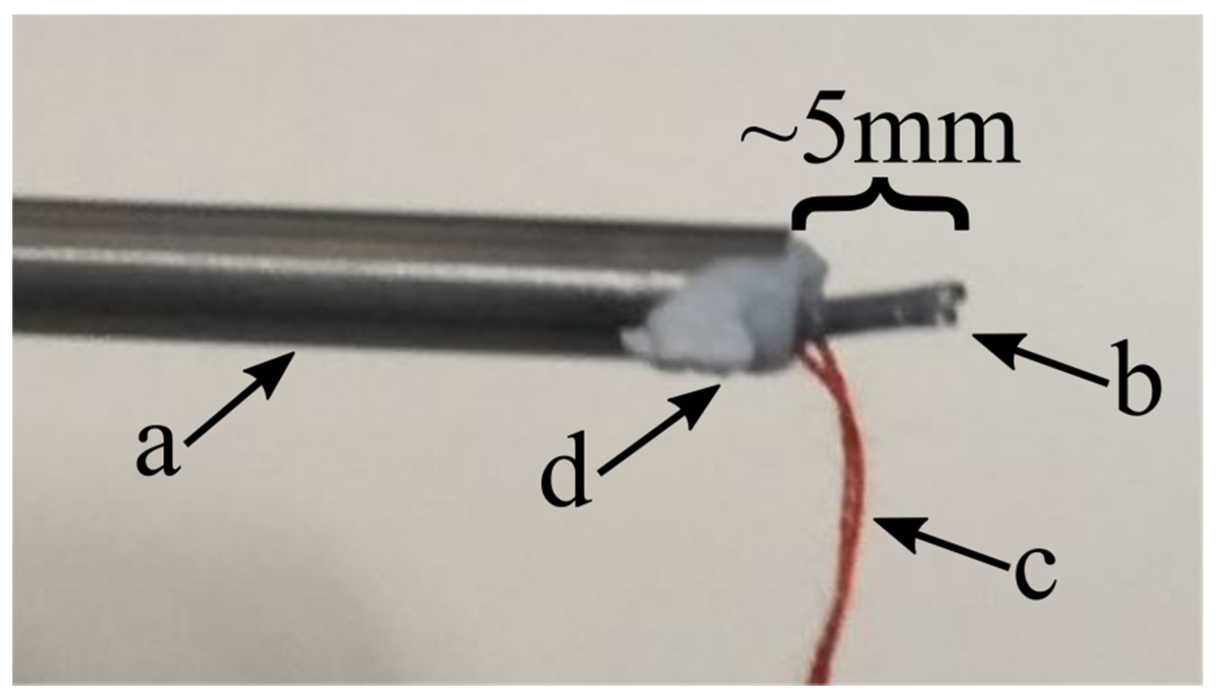
The second approach consisted of an objective evaluation of the arthroscope location detected by the algorithm. A staple connected to a thread was attached to the tip of the arthroscope with a pressure sensitive adhesive (
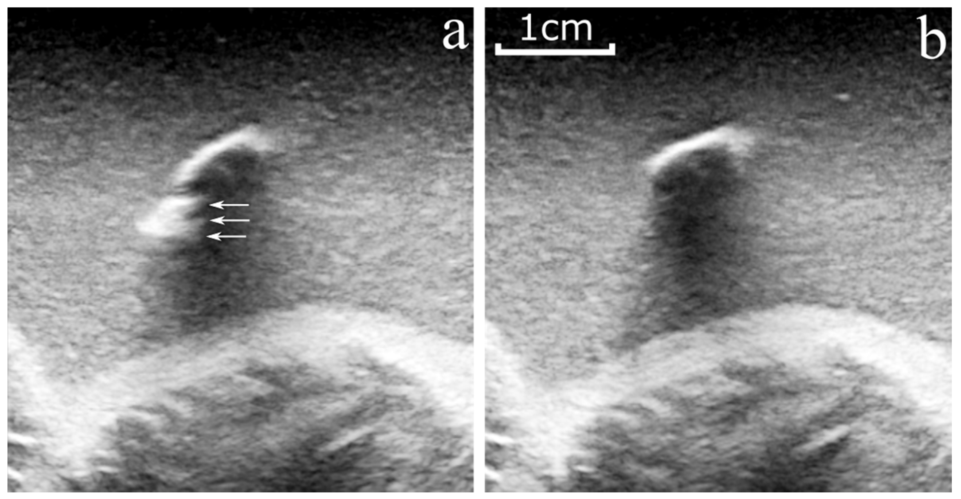
Figure 3). During US imaging, both the arthroscope and the US probe were fixed to the phantom plastic container. A first US volume was acquired with the staple attached to the arthroscope tip (
Figure 4a). The thread was then pulled to remove the staple from the arthroscope, without changing the US probe and arthroscope configuration. A second US volume was then acquired (
Figure 4b). The US volume with the staple (
Figure 4a) was used to create a pseudo ground truth for the tip of the arthroscope, as it was easier to accurately segment the staple in 3D compared to the arthroscope tip. The second US volume without the staple (
Figure 4b) was used as input to the network.
To provide precise localization in 3D instead of in 2D, the CAMs of the 2D images of the volume were generated and combined to reconstruct a 3D CAM volume. Subsequently, the 3D CAM volume was binarized by setting all voxels with a value larger than 0.2 times the maximum value in the CAM volume to 1 (as done by Zhou et al. [
35]). After creation of the binary CAM volume, the Python package Pyobb (implementation of the algorithm of Gottschalk et al. [
36]), was used to fit a bounding box encompassing all the points in the binary volume. Finally, the shortest distance between the centroid of the staple segmentation and the bounding box was calculated. The staple was sticking out from the tip of the arthroscope by roughly 5 mm (see
Figure 3), so the centroid of the staple was expected to be 2.5 mm from the arthroscope tip. Therefore, if the shortest distance between the centroid of the staple and the bounding box was smaller than 2.5mm, it was considered evidence that the tip of the arthroscope was encompassed by the bounding box. This performance metric was calculated for four US volumes (Phantom type 6 through 8). The performance of the neural network was also evaluated on a US volume of a human cadaver knee to test the arthroscope localization performance in human tissue. The evaluation was conducted using the same visual inspection method as was used for the phantom volumes. In the cadaver US volume, the arthroscope was visible as an oblong structure in a different plane. Therefore, different (automated) pre-processing steps were necessary. The 2D images were rotated by 90 degrees, cropped and padded to match the input image dimensions of the network.
3. Results
The classification (arthroscope presence in 2D US images) accuracy of the algorithm was on average 88.6% with a standard deviation of 2.4% (range: 85.5–93.5%).
Figure 5 shows an example of a true positive, false positive and false negative for the best performing cross-validation fold.
Table 3 shows the confusion matrices for the best and worst performing cross-validation fold. Both have a low number of false positives: 13 and 8, respectively. The primary performance difference between these folds was due to the number of false negatives obtained (41 vs. 111 2D US images). US volumes 42 and 65, which are present in the test set of both folds, account for 53 out of 70 additional false negatives. The number of false negatives in volume 42 and 65 was 2 and 9 for the best fold, and 30 and 34 for the worst fold, respectively.
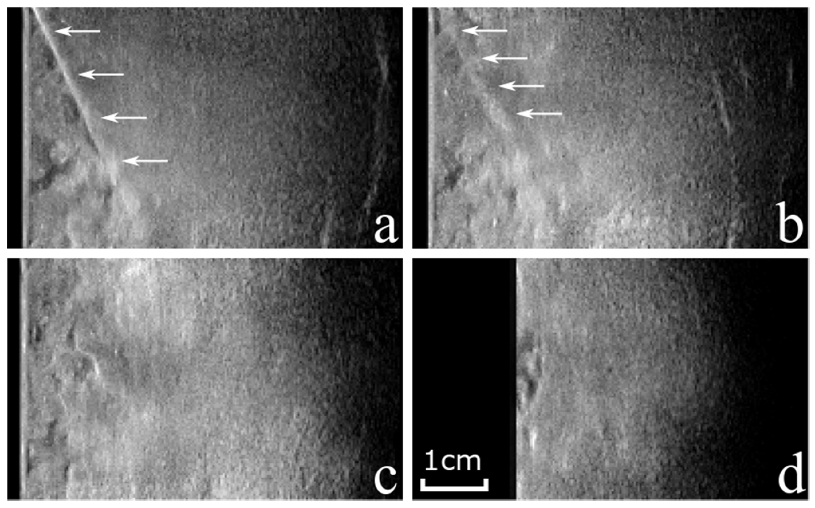
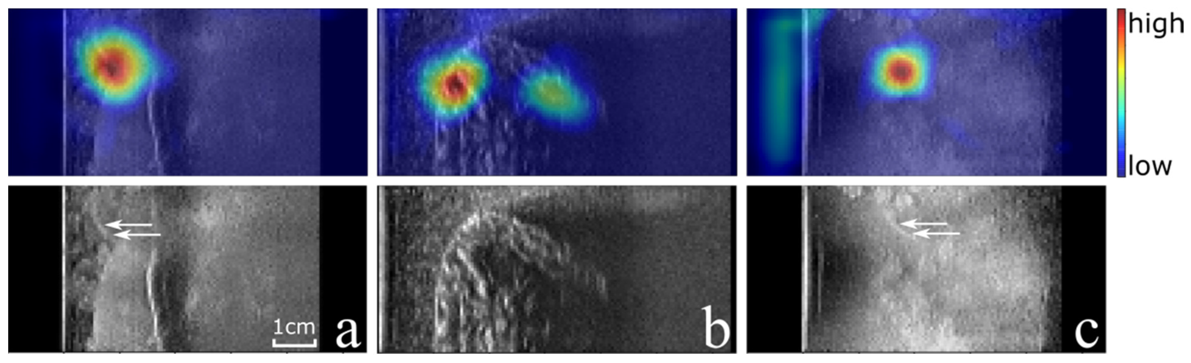
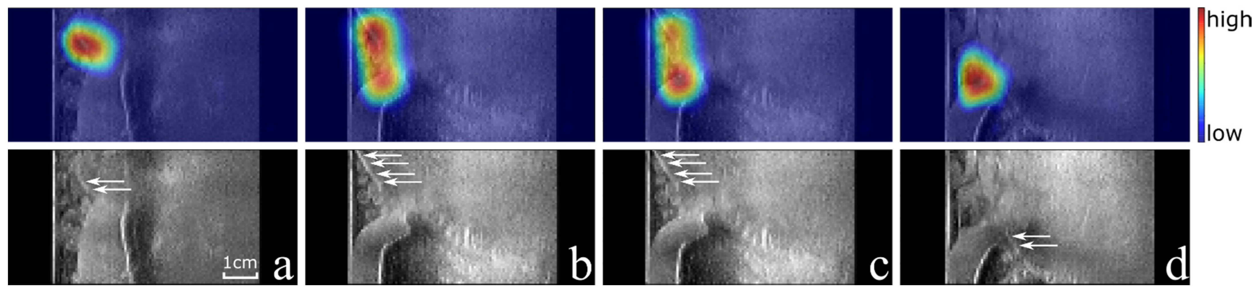
Based on the visual inspection of the CAMs of the best and worst folds by three reviewers, the localization of the arthroscope was correct in 375/375 (100%) and 277/300 (92%) true positive images, respectively. Examples of correct and in-correct localizations of the CAMs are shown in
Figure 6a–d, respectively. The creation of each CAM took 0.31 s on average.
For three out of the four US volumes, the centroid of the staple segmentation was within the bounding box drawn based on the CAMs. For the remaining US volume, the shortest distance between the bounding box drawn based on the CAMs and the staple segmentation was 0.2 mm. These results fall within the expected 2.5 mm shortest distance as described in the final paragraph of the ‘Materials and Methods chapter’.
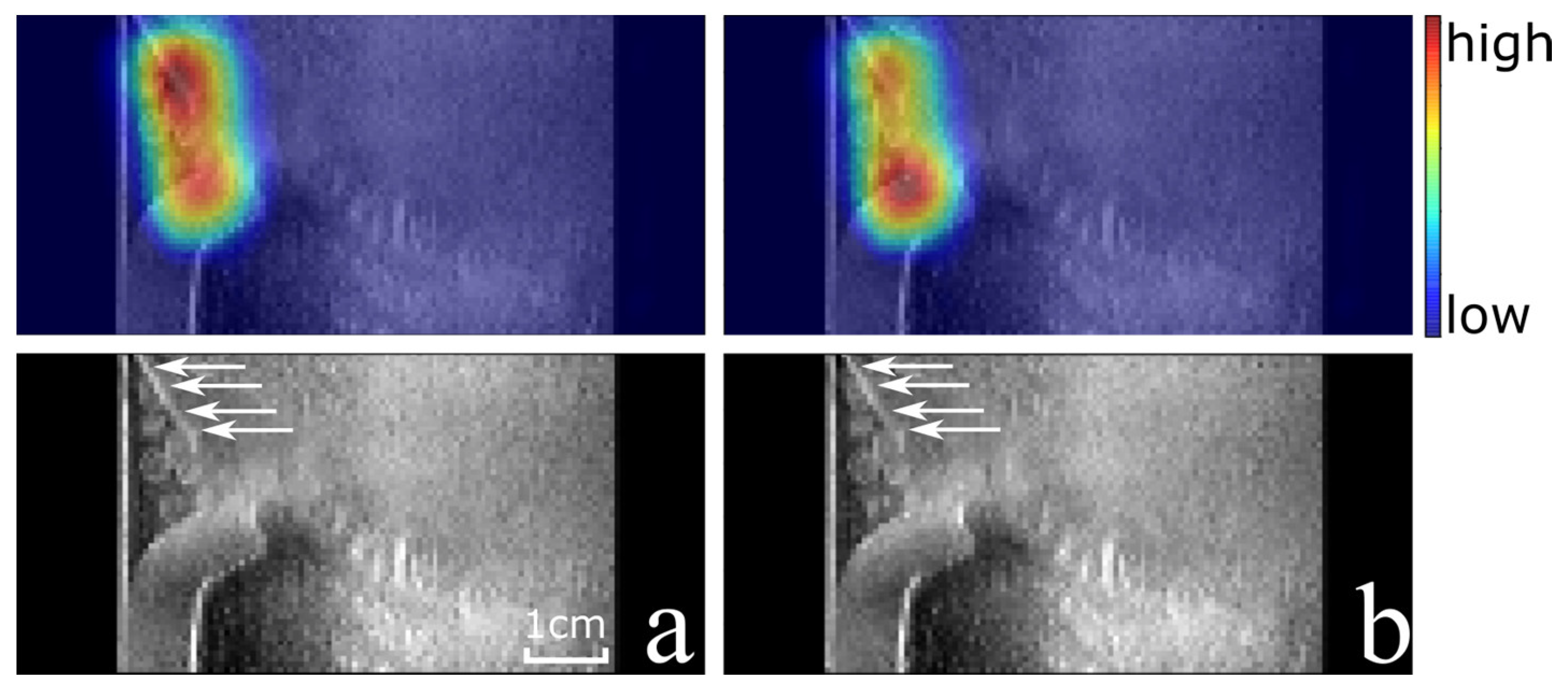
Finally, the algorithm was also evaluated on a cadaver US volume in which a classification accuracy of 83% was obtained. Out of the seven 2D images with an arthroscope, six were correctly classified and the localization was correct in 100% of these true positive cases. Out of the 107 2D images without an arthroscope, 17 were classified incorrectly (false positive).
Figure 7a shows an example of a correctly classified US image with correct localization, while
Figure 7b shows an example of a false positive classification.
4. Discussion
In this work, a weakly supervised deep-learning algorithm for the localization of an arthroscope in US volumes was presented that only requires an image-level label for each 2D image of a 3D US volume. The algorithm is capable of classifying the presence of an arthroscope in phantom US images with an accuracy of 88.6% and a standard deviation of 2.4%, which indicates it is able to generalize well. The capability of localizing the arthroscope is illustrated by the very high ratio of images in which the CAMs indicate the location correctly (100% for the fold with the highest classification accuracy). Even in challenging conditions, such as
Figure 5a, where the brightness of the arthroscope is comparable to the surrounding pixels and other bright(er) structures are present in the volume as well, the algorithm is capable of localizing the arthroscope. Furthermore, the distance between the bounding box drawn based on the class activation maps and the centroid of the staple (attached to the tip of the arthroscope) is 0.2 mm or smaller. This implies that the tip of the arthroscope is within the bounding box, and the localization performance of the network is sufficient to extract a sub-volume from the original US volume based on the CAMs. Even though the arthroscope may have moved slightly when removing the staple, the tip of the arthroscope would still be inside the bounding box if the arthroscope moved less than 2.3 mm. This follows from the fact that the centroid of the staple is ~2.5 mm away from the arthroscope tip and from the results which show that the bounding box is at maximum 0.2 mm away from the centroid of the staple. Furthermore, the threshold used to binarize the CAMs could be tuned to always capture the arthroscope entirely.
The extracted sub-volume could be input for a segmentation algorithm, or an algorithm to determine the position of the tip and orientation of the arthroscope. Thanks to the initial localization, such an algorithm would not be hampered by highly echogenic structures that lie outside the sub-volume. The output of such an algorithm could be used to register the 3D US with the 2D view of the arthroscope.
The difference in classification accuracy between the best and worst fold can be largely explained by the difference in performance for two US volumes. These volumes have the two most complex phantom compositions (Phantom type 4 and 5) which lead to challenging conditions to classify the arthroscope and may indicate the need for more training data.
Figure 5a and
Figure 6a show the results of the same image of US volume 42 for the best and worst fold which have a true positive and false negative classification, respectively. However, in both cases the CAM indicates the location of the arthroscope correctly. This shows that when the classification of the US image is not correct (the probability of an arthroscope being present is not higher than 0.5 according to the algorithm), the corresponding CAM can potentially still be used for arthroscope localization as the CAM values are significantly higher around the arthroscope than in other parts of the volume. This is also the case for the false negative example of
Figure 5c. Therefore, in future work, it will be interesting to investigate the localization accuracy of the arthroscope independently from the classification provided by the algorithm.
The ground truth labelling of the data used for network training was performed by the first author. However, a cross validation of the labels for the true positive cases was provided by three reviewers through visual inspection of the CAMs. Ideally, the performance of the algorithm should be evaluated using a segmentation of the arthroscope tip. However, obtaining a ground truth segmentation of the tip is challenging and time consuming and could possibly be affected by inter- and intra-operator variability. To obtain an objective measurement of the algorithm performance, a staple was attached to the arthroscope, which is easier to distinguish and segment. In the future, the coarse localization provided by the presented network may be used to make the segmentation of the arthroscope tip easier and less time consuming. First, a sub-volume can be extracted based on the CAM to reduce the time spent searching for the arthroscope. Secondly, the sub-volume can be sliced under an angle that agrees with the estimation of the arthroscope orientation to improve the visibility in a 2D view used for segmentation.
It is promising that the algorithm has high classification accuracy (88.3%) and that localization is correct in 100% of the true positive cases in human cadaver data (see
Figure 7). When inspecting the results of the cadaver volume more closely, 17 out of 18 false positives occurred in the first 19 2D images of the volume. On all these images a highly echogenic oblong structure created a strong response in the CAM, leading to incorrect classification. In the cadaver data, bone and tendons are visible highly echogenic on many slices of the volume, which limits the classification performance and makes the extraction of a sub-volume around the arthroscope difficult. It is important to note that none of the false positives were related to the presence of the hook-like surgical tool that was inserted into the cadaver knee as well.
An aspect that has not been studied in detail in this work is the capability to use the algorithm in real-time and provide timely feedback to the surgeon during a knee arthroscopy. When using a standard laptop only ~three images per second can be generated. Therefore, future work will be needed to reduce the required computational time. This can, for example, be conducted by using different hardware dedicated to this task, and the code can potentially be optimized to this end as well.
A limitation of this study is that the network was trained and evaluated on only 71 volumes of phantom data and only one cadaver volume was used for further evaluation. However, this proof-of-concept shows that when training on phantom data, the model is capable of detecting the arthroscope in a cadaver US volume as well. This result shows that the network has the capability of transfer learning for detecting the arthroscope, which allows the network to be pre-trained on phantom data that can be easily obtained. Future work should focus on fine tuning the network on human data and should include an extensive evaluation on US data acquired during real knee arthroscopy scenarios.
The limitations of this study can be addressed in future work in two ways. First, one should train the network on (a large amount of) human cadaver data to account for differences between the phantom data and data from an actual knee. Secondly, one should incorporate a 3D approach for detection that can utilize information of neighboring slices to distinguish an arthroscope from other highly echogenic structures. At the same time, a 3D approach can overcome the limitation of having to slice the volume in the plane where the arthroscope is visible as an oblong structure.


 ,
, 


