Theoretical Modeling and Vibration Isolation Performance Analysis of a Seat Suspension System Based on a Negative Stiffness Structure

Abstract

In this study, to improve the vibration isolation performance of a cab seat and the ride comfort of the driver, we propose a mathematical model for a seat suspension system of a construction machinery cab based on a negative stiffness structure (NSS). First, a static analysis of a seat suspension system is conducted and the different parameters and their influences on the dynamic stiffness are discussed. Thereby, the ideal configuration parameter range of the suspension system is obtained. Moreover, the nonlinear dynamic model of the designed seat suspension system is established. The frequency response and the stability are analyzed by using the HBM method and numerical simulation. The vibration transmissibility characteristics and vibration suppression effects of the seat suspension system are presented in detail. The results show that, as compared with a quasi-zero-stiffness system, the QZS-IE system has higher vibration suppression advantages under large excitation and small damping, as well as lower transmissibility and a wider vibration isolation frequency range. In addition, an inerter element with a larger mass ratio and relatively shorter distance ratio is better for vibration isolation performance of the QZS-IE system in a practical engineering application. The results of this study provide a scientific basis for the design and improvement of a seat suspension system.

1. Introduction

In recent years, with road traffic continuously improving, more and more attention has been given to ride comfort and human-centered design of vehicle seats, especially, construction machinery such as modern construction transport vehicles, in which cab seats vibrate with various degrees during vehicle operation [1]. Traditional studies have mainly focused on vibration isolation of engines and vehicle-mounted equipment on construction machinery [2,3,4]. However, drivers work in an environment of forced vibration for long periods of time, which can cause fatigue and lead to frequent accidents. Drivers’ mental and physical health can also be seriously affected. Studies have shown that cervical, spinal, and pelvis injuries occur frequently [5,6,7,8,9]. Thus, studies on the development and design of seat suspension systems are closely related to peoples’ lives. Advocating for the development of a people-oriented vehicle seat suspension system that fully considers drivers’ physical feelings and strengthens the protection of drivers would improve the working environment.

The vibration isolation mechanism of a parallel spring with a negative stiffness structure is a new type of nonlinear vibration isolation device which can significantly improve the vibration isolation effect, especially the low-frequency vibration isolation effect. Eijk J. V. et al. [10] first used negative stiffness in the mechanical design of a leaf spring to reduce the total stiffness of the system. South Korean researchers Lee C. M. et al. [11] developed a seat vibration isolation mechanism with negative stiffness based on a thin shell theory with theoretical derivation and experimental verification, which achieved good results. Yang et al. [12] studied the dynamics and power flow behavior of a nonlinear vibration isolation system with a negative stiffness mechanism, derived the nonlinear dynamic equations of the system, and obtained the frequency response function of the system under harmonic excitation by using the average method. Han et al. [13] used a type of bending mounted spring roller mechanism as a negative stiffness calibrator in parallel with a vertical linear spring to design a passive nonlinear isolator, and analyzed the dynamic characteristics of the isolator. Fan Yuanqing et al. [14] developed a vibration absorber of positive and negative stiffness elastic elements in parallel using the principle of counteracting each other, in which its stiffness was arbitrarily low. Zhang Jianzhuo et al. [15] studied a new type of vibration isolation system with positive and negative stiffness in parallel, which had higher support stiffness and lower motion stiffness. The natural frequency could be reduced by adjusting the magnitude of force at both ends of the negative stiffness mechanism and the vibration isolation effect was improved significantly. Ji Han et al. [16] proposed a new type of vibration isolation system with a negative stiffness damping device (NSD) attached to an ordinary vibration isolation layer, and discussed the effect of the NSD on the performance of the vibration isolation system. In recent years, many studies have been conducted on negative stiffness structures [17,18,19,20,21,22,23,24,25]. However, there are few in-depth studies in the literature on the negative stiffness structure for cab seats of construction machinery vehicles. Therefore, there is a need to design an accurate seat suspension system with NSS characteristics and to determine the most ideal parameters of the system according to the space size of the cab seat, and to analyze its dynamic characteristics.

In this study, the static analysis and dynamic analysis of a cab seat suspension system based on a negative stiffness structure are presented. First, the theoretical model of a seat suspension system is established, and different structural parameters and their influences on dynamic stiffness are subsequently discussed in order to determine the most ideal configuration of the parameter range of the suspension system. In addition, a nonlinear dynamic model of a quasi-zero-stiffness system with inerter elements (QZS-IE) is established, and the primary response and the stability are analyzed. The vibration suppression effects of the QZS-IE system and parameter studies are described by comparing the QZS-IE system with a quasi-zero-stiffness system. The results should accelerate the application of the QZS-IE system in construction machinery cab seats and improve the ride comfort of drivers.

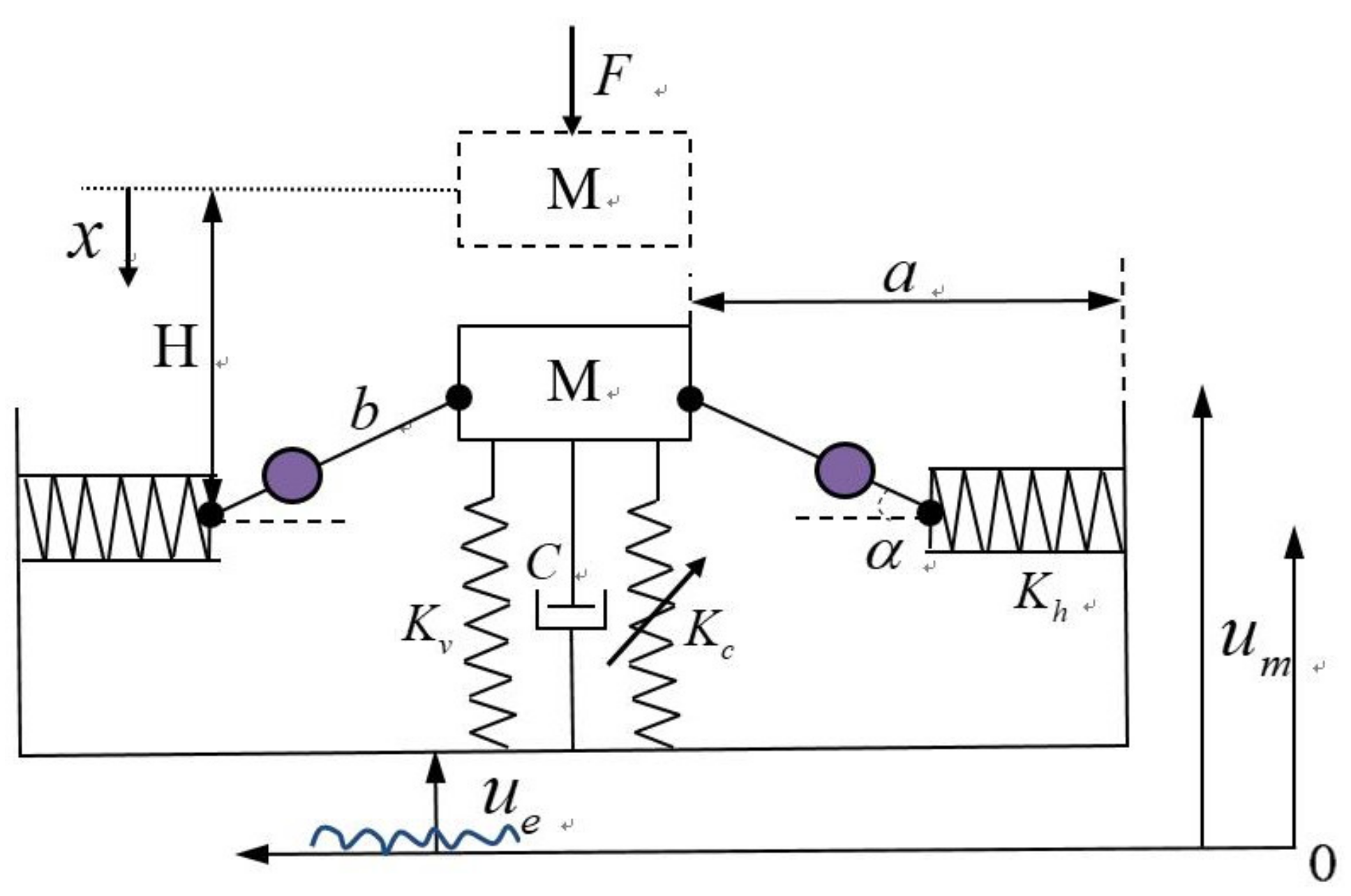
2. Model Description of Seat Suspension

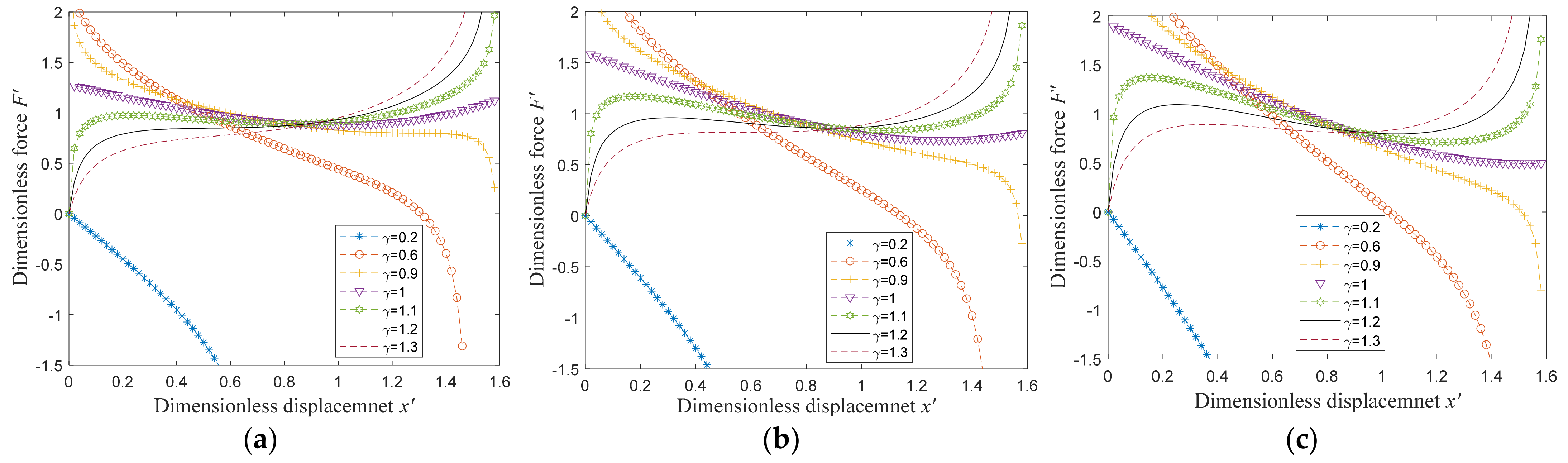
The vehicle cab seat model consists of three parts: the seat suspension system, the seat structure frame, and the driver, as shown in Figure 1. In order to investigate the dynamic characteristics of the seat suspension system specifically, the weight of the seat and human body is simplified into a rigid mass block M, and the elasticity of the cushion, the damping inside the human body, the weight of the connecting rod and joint, etc. are neglected. The simplified model contains two symmetrical negative stiffness structures, dampers, the mass block, and the supporting spring in a vertical direction, as shown in Figure 2. Moreover, two additional tunable inerter elements are attached on the two rods symmetrically; $m_a$ is the mass of the inerter element, and the location of the attached inerter element can be adjusted to achieve a better vibration isolation performance of the seat structure. The rotation freedom of the seat structure is limited, and the seat can only move in a vertical direction. The vibration reduction amount of the suspension system is affected by different parameters, such as spring stiffness, the damping coefficient, and length of the connecting rod.

3. Static Analysis

3.1. Theoretical Model

In Figure 2, $K_v$ and $K_{\mathrm{H}}$ represent vertical spring stiffness and horizontal spring stiffness, respectively; $L_0$ represents the original length of horizontal spring; $L_{\mathrm{H}}$ represents the length of horizontal spring at any position; $F$ represents the elastic restoring force of the vibration-isolated object; $b$ represents the length of connecting rod between horizontal spring and mass block; $a$ represents the distance from the isolated equipment M to the fixed end of horizontal spring. The initial state of the mass block is the position of the dashed frame, and each spring of the suspension system is in a compression state during vehicle operation. The dynamic stiffness of the suspension system can be adjusted by changing the above parameters.

Assuming that the spring in Figure 2 is in equilibrium, the deformation length of the horizontal spring is:

$${\Delta }_l={\Delta }_r=\sqrt{b^2-{(\mathrm{H}-x)}^2}-(a-L_0)$$

(1)

where $\mathrm{H}$ is the initial deformation of the vertical spring, obtained as:

$$\mathrm{H}=\sqrt{b^2-{(a-L_0)}^2}$$

(2)

Then, the horizontal force produced by the horizontal spring is:

$$F_{\mathrm{H}c}=2K_{\mathrm{H}}(\sqrt{b^2-{(\mathrm{H}-x)}^2}-(a-L_0))$$

(3)

To convert it to the force $F_{\mathrm{H}\mathrm{v}}$ in the vertical direction:

$$F_{\mathrm{H}v}=2K_{\mathrm{H}}(\sqrt{b^2-{(\mathrm{H}-x)}^2}-(a-L_0\left)\right)\tan \alpha$$

(4)

where $\alpha$ is the angle between the rod and the horizontal plane, obtained as:

$$\tan \alpha =\frac{\mathrm{H}-x}{\sqrt{b^2-{(\mathrm{H}-x)}^2}}$$

(5)

The force produced by the vertical spring in the vertical direction can be expressed as:

$$F_v=K_v\cdot x+K_c\cdot x^3$$

(6)

Thus, according to the principle of virtual work, the restoring force $F$ of the system in the vertical direction is obtained as:

$$F=F_v+F_{\mathrm{H}v}=K_v\cdot x+K_c\cdot x^3+2K_{\mathrm{H}}(\mathrm{H}-x)(1-\frac{a-L_0}{\sqrt{b^2-{(\mathrm{H}-x)}^2}})$$

(7)

For dimensionless treatment, introducing the structural parameters of the system are, sequentially, as follow:

$$\begin{gathered} \begin{array}{l}{F}^{\prime }=\frac{F}{K_v{L}_0},\alpha =\frac{K_{\mathrm{H}}}{K_v},\eta =\frac{K_c{L}_0{}^2}{K_v},x^{\prime }=\frac{x}{L_0}\\ {\gamma }_1=\frac{b}{L_0},{\gamma }_2=\frac{a}{L_0}\end{array} \\ {\mathrm{H}}^{\prime }=\sqrt{{\gamma }_1{}^2-{({\gamma }_2-1)}^2} \end{gathered}$$

where $F^{\prime }$ is dimensionless restoring force, $x^{\prime }$ is dimensionless displacement of polynomial. Thus, the dimensionless force–displacement relation of system is obtained, as follow:

$$F^{\prime }=x^{\prime }+\eta {x^{\prime }}^3+2\alpha ({\mathrm{H}}^{\prime }-x^{\prime })(1-\frac{{\gamma }_2-1}{\sqrt{{\gamma }_1^2-{({\mathrm{H}}^{\prime }-x^{\prime })}^2}})$$

(8)

Then, by differentiating Equation (8) the relationship between the dimensionless dynamic stiffness $K^{\prime }$ and displacement $x^{\prime }$ of system is obtained as:

$$K^{\prime }=1+3\eta {x^{\prime }}^2-2\alpha (1-\frac{{{\mathrm{H}}^{\prime }}^2({\gamma }_2-1)-2{\mathrm{H}}^{\prime }({\gamma }_2-1)x^{\prime }+({\gamma }_2-1){x^{\prime }}^2}{{\left({\gamma }_1{}^2-{({\mathrm{H}}^{\prime }-x^{\prime })}^2\right)}^{3/2}}-\frac{{\gamma }_2-1}{\sqrt{{\gamma }_1{}^2-{({\mathrm{H}}^{\prime }-x^{\prime })}^2}})$$

(9)

According to Equation (9), it can be seen that there are four design parameters $\alpha$, ${\gamma }_1$, ${\gamma }_2$, $\eta$, and their variation can have the influence on the dynamic stiffness of system.

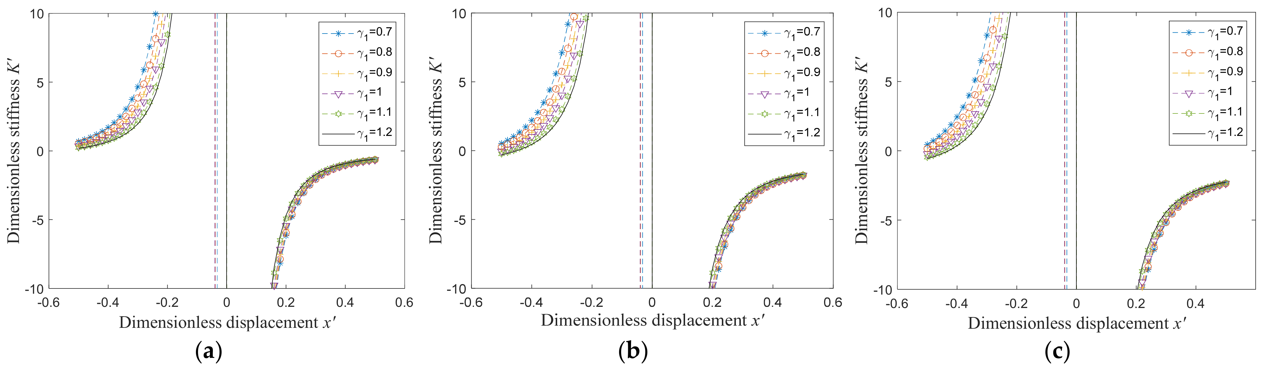
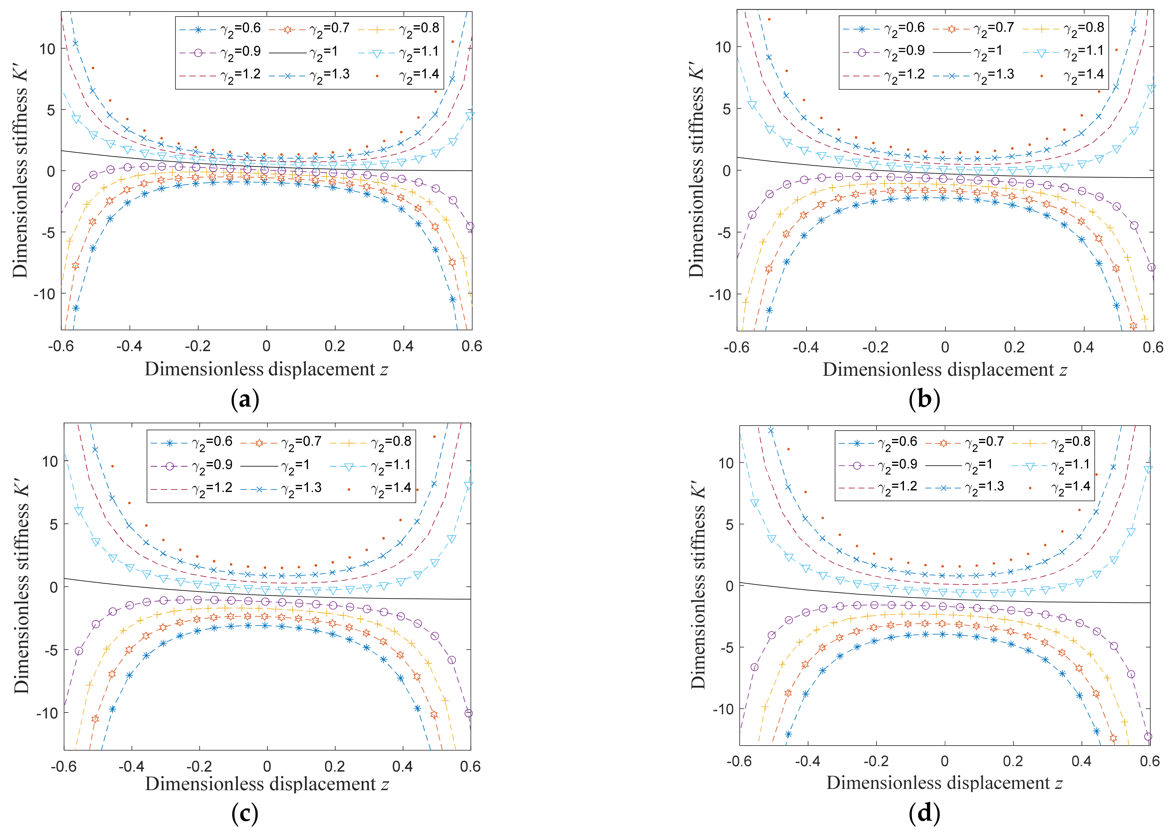
3.2. Quasi-Zero-Stiffness (QZS) Conditions

Letting ${\mathrm{H}}^{\prime }-x^{\prime }=0$, the dimensionless equivalent stiffness of the suspension system at the static equilibrium position is given by:

$${K^{\prime }}_{eq}=1+3\eta {{\mathrm{H}}^{\prime }}^2-2\alpha (\frac{{\gamma }_1-{\gamma }_2+1}{{\gamma }_1})$$

(10)

${K^{\prime }}_{eq}$ may be larger or smaller than zero. However, the QZS conditions of the suspension system can be obtained by letting the dynamic stiffness ${K^{\prime }}_{eq}$ and the second derivation $\frac{d^2{K^{\prime }}_{eq}}{d{x^{\prime }}^2}$ be equal to zero.

Under these two conditions, $\alpha =1/4$ is obtained which can make the QZS range wider around the equilibrium position, approximately like a horizontal straight line. In addition, some existing parameter combinations will lead to the inflexion points of ${K^{\prime }}_{eq}$ at the static equilibrium position, so that the lower QZS in a wide region could be generated. The second derivative of dynamic stiffness of the suspension system is always larger than zero. It is worthwhile noting that the design of the parameters $\alpha$, ${\gamma }_1$, ${\gamma }_2$, $\eta$ could be achieved according to a practical application. Among the four independent parameters, $\alpha$ represents the stiffness ratios and $\eta$ is the combination of stiffness ratio and structural dimension; both ${\gamma }_1$ and ${\gamma }_2$ are the structural dimension ratio. Thus, by considering space dimensions of construction machinery cab and different working conditions, the values of parameters $\alpha$, ${\gamma }_1$, ${\gamma }_2$, $\eta$ can be readily realized and optimized.

3.3. Parameter Analysis

Different parameters have different influences on a suspension system. In order to evaluate the mechanical properties of the system, the value ranges for parameters need to be further determined. The dimensionless force–deflection characteristic curves under different values of $\alpha$ are shown in Figure 3. With an increase in the value of $\alpha$, the curvature of the curve is changed. Among these curves, the flatness degree of the curve is even higher at $0.6<\alpha <1$.

As shown in Figure 4, by MATLAB numerical calculation, it can be found that with an increase in displacement, the restoring force curve of the system is on a downward trend, and the proposed structure has obvious negative stiffness characteristics. When ${\gamma }_1<1$, the occurrence time of the first peak of the curve is faster and the change of the corresponding displacement is smaller. When ${\gamma }_1\ge 1$, the force change trend of the system in the vertical direction is gentle, which indicates that the seat has better vibration isolation performance, and the selection of the NSS parameters is ideal. It is found that the dimensionless force $F^{\prime }$ of the system peaks in a short time period when the value of ${\gamma }_1$ is especially small. Therefore, this situation should be avoided to occur when designing parameters so as not to affect the dynamic characteristics of the suspension system. In addition, by contrasting and analysis, the results show that a change in $\alpha$ affects the trend of the overall force change of the system. With an increase in $\alpha$, the force change trend accelerates, indicating that the vibration amplitude of the seat in the vertical direction increases which reduces the driver′s ride comfort. Therefore, it is recommended that $\alpha$ not take a larger value, and rather, try to make the stiffness of the horizontal spring smaller than that of the vertical spring.

Figure 5 shows the dimensionless force–deflection characteristic curves with different values of ${\gamma }_2$. The results show that when the value of ${\gamma }_2$ is greater than 1, curve changes vary regularly, which is similar to an elongated sinusoidal curve, with existing maximum and minimum peak values. It indicates that the dimensionless force $F^{\prime }$ between the two peaks decreases with an increase in displacement, and inversely in the other positions, the value of $F^{\prime }$ increases with an increase in displacement. However, when the value of ${\gamma }_2$ is less than 1, the initial value of the dimensionless force $F^{\prime }$ begins to change irregularly, and the value of $F^{\prime }$ decreases with an increase in displacement. In this case, although the stiffness of the suspension system is negative stiffness, it is not suitable for the design of the above negative stiffness model structure. When ${\gamma }_2$ < 1, the shape of stiffness curve is convex parabola, and the stiffness reaches the maximum peak value in the static equilibrium position. However, when it is distant enough from the static equilibrium position, the stiffness of the system is always negative, and the vibration isolation system is in an unstable state.

Considering the nonlinear characteristics of the suspension system and multiple design parameters, the dimensionless dynamic stiffness of the system should be used to evaluate the vibration isolation system so that the appropriate suspension configuration parameters can be selected. As can be seen in Figure 6, as the value of ${\gamma }_1$ becomes larger, the basic outline of the stiffness characteristic curves of system does not change obviously, while the curvature of the stiffness characteristic curve changes. For dimensionless displacement $x^{\prime }$ < 0, when the value of $\alpha$ increases, the absolute values of stiffness of the suspension system also increases. For dimensionless displacement $x^{\prime }$ > 0, when the value of $\alpha$ increases, the curve moves to the right overall, and the suspension system deviates from the quasi-zero stiffness more and more. It also illustrates that the value of the parameter $\alpha$ should not be too large.

From Figure 7, the corresponding stiffness curves under different values are nearly symmetric at z = 0. When ${\gamma }_2$ ≥ 1.2, the dynamic stiffness curve is a concave parabola shape, and the stiffness value at static equilibrium position is the smallest; when $0.9\le {\gamma }_2<1.2$, the stiffness value is unstable with varying between positive and negative. Therefore, the configuration of structural parameters needs to be reasonably selected to make the dynamic stiffness of the static equilibrium position zero or greater than zero. Additionally, when ${\gamma }_2$ = 1 and $\alpha$ = 1.2, its dynamic stiffness curve is an oblique line with a tiny angle, and the stiffness value can be considered to be $K^{\prime }=-1$. This situation shows that the distance from the isolated equipment to the static equilibrium position can be infinite, and dynamic stiffness of the region above the line $K^{\prime }=-1$ is always less than static stiffness. However, in the case of ${\gamma }_2$ > 1, the infinite range, from the isolated equipment to the static equilibrium position, decreases with increases in the values of ${\gamma }_2$.

Figure 7 also shows several sets of stiffness curves corresponding to different values of $\alpha$. Through a comparison, it can be concluded that when $\alpha =0.5$ and ${\gamma }_2$ ≥ 1.2, the dynamic stiffness of the system around the static equilibrium position is very close to zero, that is, near quasi-zero stiffness. This illustrates that the selection of parameters $\alpha$ and ${\gamma }_2$ has a certain impact on the stiffness characteristics of the system.

Furthermore, the dynamic stiffness curves of the system under different variations of $\alpha$ are shown in Figure 8. It can be seen that as the value of $\alpha$ increases, the minimum value of the dimensionless stiffness curve decreases. When $\alpha$ = 1.2 and $\alpha$ = 1.4, the system is close to quasi-zero stiffness, but the concave parabola is closer to the center axis. The correctness of the above ${\gamma }_2$ ≥ 1.2 analysis results is verified again. The larger the range of displacement changes for the suspension system, the better the vibration isolation effect. To sum up, the design parameters of the suspension system $1.2\le {\gamma }_2\le 1.4$ and $\alpha$ = 0.5 are the most ideal configuration parameters of the system. However, in the actual design process, it is difficult to obtain these accurate values because of errors in manufacturing and assembly, and ${\gamma }_2$ < 1.2 may also appear, therefore, the quasi-zero stiffness should be satisfied as far as possible during the design.

4. Dynamic Analysis

4.1. Dynamic Modeling of the Proposed Seat Suspension

With respect to the seat suspension system, $u_m(t)$ is the absolute displacement of the isolated equipment in space. When the isolated equipment M experiences upward a vertical displacement $z$ from its initial position, the kinetic energy $T$ of the system is:

$$T=\frac{1}{2}M{\dot{u}}_m^2+m_a{v}_a^2$$

(11)

where

$$v_a=\sqrt{{\left[\frac{d(\lambda x)}{dt}\right]}^2+{\left[\frac{d\left((1-\lambda )\sqrt{b^2-{(\mathrm{H}-x)}^2}-(1-\lambda )(a-L_0)\right)}{dt}\right]}^2}=\dot{x}\sqrt{{\lambda }^2+{(1-\lambda )}^2\frac{{(x-\mathrm{H})}^2}{b^2-{(\mathrm{H}-x)}^2}}$$

(12)

The vertical upward external excitation from the base is $u_e(t)$. The relative vertical motion is $z(t)=u_m(t)-u_e(t)$. $z$ is the displacement of the isolated equipment relative to the base of the cab:

$$z=\mathrm{H}-x$$

(13)

The relative velocity and acceleration of the isolated equipment are, respectively, defined as below:

$$\dot{z}={\dot{u}}_m-{\dot{u}}_e$$

(14)

$$\ddot{z}={\ddot{u}}_m-{\ddot{u}}_e$$

(15)

The potential energy of the system contains the elastic potential energy of the vertical springs and the two springs in horizontal direction, which is as:

$$V=\frac{1}{2}{k}_l{\Delta }_l^2+\frac{1}{2}{k}_r{\Delta }_r^2+\frac{1}{2}{k}_v{\Delta }_x^2+\frac{1}{4}{k}_c{\Delta }_x^4+Mg\cdot x+2m_{a}g\lambda {\Delta }_x$$

(16)

The dissipation function $D$ is given by:

$$D=\frac{1}{2}{C}_l{\dot{\Delta }}_l^2+\frac{1}{2}{C}_r{\dot{\Delta }}_r^2+\frac{1}{2}{C}_v{\dot{\Delta }}_x^2=\frac{1}{2}{C}_v{({\dot{u}}_m-{\dot{u}}_e)}^2$$

(17)

where $C$ is the damping coefficient ($N/m/s$), $k$ is the spring stiffness ($N/m$), $\Delta$ is the variation of the spring length, $\dot{\Delta }$ is the relative velocity at both ends of the spring ($m/s$), Subscripts $l$, $r$ and $v$, respectively, represent the left, right, and vertical direction of the suspension system. $\lambda$($0\le \lambda \le 1$) is the distance ratio. Since the system is symmetrical structure, it is considered that $k_l=k_r=K_{\mathrm{H}}$, $C_l=C_r$, ${\Delta }_l={\Delta }_r$. For the model of this suspension system, the damping in the horizontal direction is designed to be $C_l=C_r=0$. Note that the weight of the isolated equipment M and the two attached inerter elements can be offset by the precompression of the vertical spring. So, we can have:

$$K_v{\Delta }_s+K_c{\Delta }_s^3=Mg+2\lambda m_{a}g$$

(18)

$${\Delta }_x=x+{\Delta }_s$$

(19)

where ${\Delta }_s$ is the precompression of the vertical spring.

Applying the Lagrangian Equation of the second kind, it can be expressed as:

$$\frac{d}{dt}\left(\frac{\partial T}{\partial {\dot{u}}_m}\right)-\frac{\partial }{\partial u_m}(T-V)=Q_x$$

(20)

where $Q_x$ comprises of the excitation force $F_e$ and the damping force introduced to account for energy dissipation, and it can be expressed as:

$$Q_x=F_e-\frac{\partial D}{\partial u_m}$$

(21)

By substituting Equation (12) into Equation (11), substituting Equations (18) and (19) into Equation (16), and then substituting the expressions of potential energy, kinetic energy into the Lagrange Equation (20), the dynamic equation of the system can be derived as follows:

$$\left\{1+2\frac{m_a}{M}\left[{\lambda }^2+\frac{{(1-\lambda )}^2{z}^2}{b^2-z^2}\right]\right\}\ddot{z}-2\frac{m_a}{M}\frac{{(1-\lambda )}^{2}z{b}^2}{{\left(b^2-z^2\right)}^2}{\dot{z}}^2+\frac{C}{M}\dot{z}+\frac{K_v}{M}z+\frac{K_c}{M}{z}^3+2\frac{K_{\mathrm{H}}}{M}(1-\frac{a-L_0}{\sqrt{b^2-z^2}})z=-{\ddot{u}}_e$$

(22)

where ${\Delta }_s$ and gravity terms no longer exist due to Equations (18) and (19).

The left-hand side of the equation of motion includes damping term and restoring force term, respectively, which are the same as those of the equivalent quasi-zero-stiffness (QZS) system without the attached inerter elements. From Equation (22), it also can be seen that the nonlinear stiffness term and the inertia term have nonlinear characteristics. The structural parameters of the system can be adjusted to satisfy different engineering requirements. Especially when the construction machinery is excited by larger amplitude, the vibration peak transmissibility rate can be further reduced by adjusting the parameter of the nonlinear inerter $\lambda$.

For the QZS vibration isolation system in Figure 2, assuming that the base displacement excitation is:

$$u_e=U_e\cos (\omega t)$$

(23)

By introducing the dimensionless parameters as:

$$\begin{gathered} \overline{z}=\frac{z}{b}, \mu =\frac{m_a}{M}, \beta =\frac{k_h}{k_v}, \epsilon =\frac{k_c{b}^2}{k_v}, \\ {\gamma }_1=\frac{b}{L_0}, {\gamma }_2=\frac{a}{L_0}, \delta =\frac{a}{b}, \zeta =\frac{c}{2m{\omega }_0}, u_0=\frac{U_e}{k_{v}b} ,{\omega }_n=\sqrt{\frac{k_v}{M}}, \Omega =\frac{\omega }{{\omega }_n}, \tau ={\omega }_{n}t \end{gathered}$$

Then, the dimensionless dynamic equation of Equation (12) is given by:

$$\left\{1+2\mu \left[{\lambda }^2+\frac{{(1-\lambda )}^2{\overline{z}}^2}{1-{\overline{z}}^2}\right]\right\}{\overline{z}}^{″}-2\mu \frac{{(1-\lambda )}^2\overline{z}}{{\left(1-{\overline{z}}^2\right)}^2}{({\overline{z}}^{\prime })}^2+2\zeta {\overline{z}}^{\prime }+\left[1+2\beta (1-\frac{\delta -1/{\gamma }_1}{\sqrt{1-{\overline{z}}^2}})\right]\overline{z}+\epsilon {\overline{z}}^3=u_0{\Omega }^2\cos (\Omega \tau )$$

(24)

where $(\cdot {)}^{″}=\frac{d^2(\cdot )}{d{t}^2}$, $(\cdot {)}^{\prime }=\frac{d(\cdot )}{dt}$, the Equation (14) contains some complex expressions, which increases the difficulty of the analytical response calculation. And thus, the fractional and radical expressions can be replaced by using the Taylor series expansion [26]. Then, the approximate expression of the equation of motion (24) is given by:

$$({\sigma }_1+{\sigma }_2{\overline{z}}^2+{\sigma }_2{\overline{z}}^4){\overline{z}}^{″}-({\sigma }_2\overline{z}+2{\sigma }_2{\overline{z}}^3){({\overline{z}}^{\prime })}^2+2\zeta {\overline{z}}^{\prime }+\frac{1}{4}({\overline{z}}^3+\frac{3}{4}{\overline{z}}^5)+2\overline{z}+\epsilon {\overline{z}}^3=u_0{\Omega }^2\cos (\Omega \tau )$$

(25)

where

$${\sigma }_1=1+2\mu {\lambda }^2$$

(26)

$${\sigma }_2=2\mu {(1-\lambda )}^2$$

(27)

From the dimensionless dynamic Equation (24), it can be seen that there are square term and cubic term in the equation. Therefore, the solution of Equation of motion will contain constant term and harmonic series, which can reflect the vibration offset and vibration, respectively. Equation (24) can be solved in the following application of the harmonic balance method (HBM). By omitting the higher order harmonic terms, the response of the system is assumed in the form:

$$\overline{z}=A_0+A_1\cos (\Omega \tau +\phi )$$

(28)

where $A_0$ represents the offset of vibration, $A_1$ is the relative displacement amplitude, and $\phi$ is the phase between the excitation and the response. Substituting Equation (27) into (25), assuming the coefficients of the same sines and cosines terms are equal, one can obtain:

$$\left\{\begin{array}{l}(\frac{15}{128}-\frac{7}{8}{\sigma }_2{\Omega }^2)A_1{}^5+\\ \left[\frac{3}{4}(\frac{1}{4}+{\sigma }_2)-{\sigma }_2{\Omega }^2\right]A_1{}^3\\ +(2-{\sigma }_1{\Omega }^2)A_1\end{array}\right\}\cos \phi +(-2\zeta A_1\Omega )\sin \phi =u_0{\Omega }^2$$

(29)

$$-2\zeta A_1\Omega \cos \phi +\left\{\begin{array}{l}(-\frac{15}{128}+\frac{7}{8}{\sigma }_2{\Omega }^2)A_1{}^5+\\ \left[{\sigma }_2{\Omega }^2-\frac{3}{4}(\frac{1}{4}+{\sigma }_2)\right]A_1{}^3\\ +({\sigma }_1{\Omega }^2-2)A_1\end{array}\right\}\sin \phi =0$$

(30)

Squaring and adding the expressions (29) and (30) above to acquire the amplitude–frequency relation:

$${\left\{\begin{array}{l}(\frac{15}{32}-\frac{7}{2}{\sigma }_2{\Omega }^2)A_1{}^5+\left[3(\frac{1}{4}+{\sigma }_2)-4{\sigma }_2{\Omega }^2\right]A_1{}^3\\ +(8-4{\sigma }_1{\Omega }^2)A_1\end{array}\right\}}^2+64{\zeta }^2{A}_1{}^2{\Omega }^2=16u_0{}^2{\Omega }^4$$

(31)

4.2. Displacement Transmissibility

By solving Equation (31), a square equation in ${\Omega }^2$ can be required and the relationship between the response amplitude and the driving frequency can be yielded as:

$${\Omega }^4{f}_3(A_1)+{\Omega }^2{f}_2(A_1)+f_1(A_1)=0$$

(32)

where

$$f_3(A_1)=\frac{49}{4}{\sigma }_2^2{A}_1{}^{10}+28{\sigma }_2^2{A}_1{}^8+4(4{\sigma }_2^2+7{\sigma }_1{\sigma }_2)A_1{}^6+32{\sigma }_1{\sigma }_2{A}_1{}^4+16{\sigma }_1^2{A}_1{}^2-16u_0^2$$

(33)

$$f_2(A_1)=-\frac{105}{32}{\sigma }_2{A}_1{}^{10}-3{\sigma }_2(7{\sigma }_2+3)A_1{}^8-(\frac{15}{4}{\sigma }_1+62{\sigma }_2+24{\sigma }_2^2)A_1{}^6-\left[64{\sigma }_2+(6+24{\sigma }_2){\sigma }_1\right]A_1{}^4-64({\sigma }_1-{\zeta }^2)A_1{}^2$$

(34)

$$f_1(A_1)=\frac{225}{1024}{A}_1{}^{10}+\frac{45}{16}({\sigma }_2+\frac{1}{4})A_1{}^8+\left[9(\frac{1}{4}+{\sigma }_2{)}^2+\frac{15}{2}\right]A_1{}^6+(48{\sigma }_2+12)A_1{}^4+64A_1{}^2$$

(35)

The solution of Equation (21) can be expressed as:

$${\Omega }^2=\frac{105{\sigma }_2{A}_1{}^{10}/32+3{\sigma }_2(7{\sigma }_2+3)A_1{}^8+(15{\sigma }_1/4+62{\sigma }_2+24{\sigma }_2^2)A_1{}^6+\left[64{\sigma }_2+(6+24{\sigma }_2){\sigma }_1\right]A_1{}^4+64({\sigma }_1-{\zeta }^2)A_1{}^2\pm \sqrt{\Delta }}{49{\sigma }_2^2{A}_1{}^{10}/2+56{\sigma }_2^2{A}_1{}^8+8(4{\sigma }_2^2+7{\sigma }_1{\sigma }_2)A_1{}^6+64{\sigma }_1{\sigma }_2{A}_1{}^4+32{\sigma }_1^2{A}_1{}^2-32u_0^2}$$

(36)

where

$$\Delta =m_1{A}_1{}^{12}+m_2{A}_1{}^{10}+m_3{A}_1{}^8+m_4{A}_1{}^6+m_5{A}_1{}^4+m_6{A}_1{}^2$$

(37)

$$m_1=-420{\sigma }_2{\zeta }^2-54{\sigma }_1{\sigma }_2-576{\sigma }_2^2-342{\sigma }_2^2{\sigma }_1-504{\sigma }_2^3{\sigma }_1$$

(38)

$$m_2=-2688{\sigma }_2^2{\zeta }^2-1152{\sigma }_2{\zeta }^2-1080{\sigma }_1{\sigma }_2+225u_0{}^2/16$$

(39)

$$m_3=516{\sigma }_1^2-480{\sigma }_1{\zeta }^2-7936{\sigma }_2{\zeta }^2-3072{\sigma }_2^2{\zeta }^2+576{\sigma }_1^2{\sigma }_2^2+288{\sigma }_2{\sigma }_1^2-180u_0{}^2({\sigma }_2+1/4)$$

(40)

$$m_4=-64{\sigma }_2{\zeta }^2-{\zeta }^2(6{\sigma }_1+24{\sigma }_1{\sigma }_2)+64u_0{}^2(9{\sigma }_2^2+9{\sigma }_2/2+129/16)$$

(41)

$$m_5={64}^2{\zeta }^4-2^{13}{\sigma }_1{\zeta }^2+64u_0{}^2(48{\sigma }_2+12)$$

(42)

$$m_6={64}^2{u}_0{}^2$$

(43)

Letting ${\Omega }_1={\Omega }_2$, the maximum displacement response amplitude ${\overline{z}}_{\max }$ can be obtained when:

$$m_1{A}_1{}^{12}+m_2{A}_1{}^{10}+m_3{A}_1{}^8+m_4{A}_1{}^6+m_5{A}_1{}^4+m_6{A}_1{}^2=0$$

(44)

The corresponding resonant frequency ${\Omega }_{\max }$ at the maximum displacement response amplitude can be yielded as:

$${\Omega }_{\max }=\frac{105{\sigma }_2{\overline{z}}^{10}{}_{\max }/32+3{\sigma }_2(7{\sigma }_2+3){\overline{z}}^8{}_{\max }+(15{\sigma }_1/4+62{\sigma }_2+24{\sigma }_2^2){\overline{z}}^6{}_{\max }+\left[64{\sigma }_2+(6+24{\sigma }_2){\sigma }_1\right]{\overline{z}}^4{}_{\max }+64({\sigma }_1-{\zeta }^2){\overline{z}}^2{}_{\max }}{49{\sigma }_2^2{\overline{z}}^{10}{}_{\max }/2+56{\sigma }_2^2{\overline{z}}^8{}_{\max }+8(4{\sigma }_2^2+7{\sigma }_1{\sigma }_2){\overline{z}}^6{}_{\max }+64{\sigma }_1{\sigma }_2{\overline{z}}^4{}_{\max }+32{\sigma }_1^2{\overline{z}}^2{}_{\max }-32u_0^2}$$

(45)

Given that the absolute displacement transmissibility is the common index to evaluate the performance of vibration isolation systems [27]. Therefore, the absolute displacement transmissibility is defined as the ratio of the magnitude of the absolute displacement of the QZS vibration isolation system to the base as:

$$T=20\log \frac{\left|u_m\right|}{\left|u_e\right|}=\frac{\sqrt{A_1{}^2+U_e{}^2+2A_1{U}_e\cos \phi }}{U_e}$$

(46)

Combining with Equations (28) and (29), substituting $\cos \phi$ into Equation (46), then, the absolute displacement transmissibility is expressed as:

$$T=20\log \frac{\left|u_m\right|}{\left|u_e\right|}=20\log \sqrt{1+\frac{A_1{}^2}{U_e{}^2}+\frac{A_1\Lambda }{U_e{}^2}}$$

(47)

where

$$\Lambda =(\frac{15}{64}-\frac{7}{4}{\sigma }_2{\Omega }^2)A_1{}^5+\left[\frac{3}{2}(\frac{1}{4}+{\sigma }_2)-2{\sigma }_2{\Omega }^2\right]A_1{}^3+(4-2{\sigma }_1{\Omega }^2)A_1$$

(48)

In the case of small amplitude excitation, the degree of nonlinearity of dynamic equation will be weak so that the dynamic Equation (22) can be linearized [28]. Thus, by the linear vibration theory the transmissibility can be given as:

$$T=20\log \sqrt{\frac{1+(2\zeta \Omega {)}^2}{{(1-{\Omega }^2)}^2+{(2\zeta \Omega )}^2}}$$

(49)

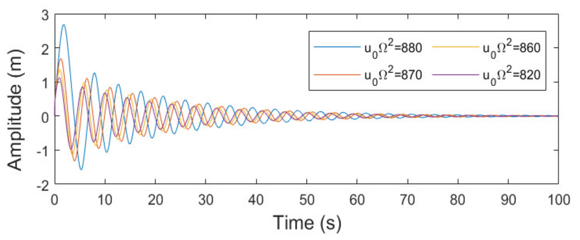
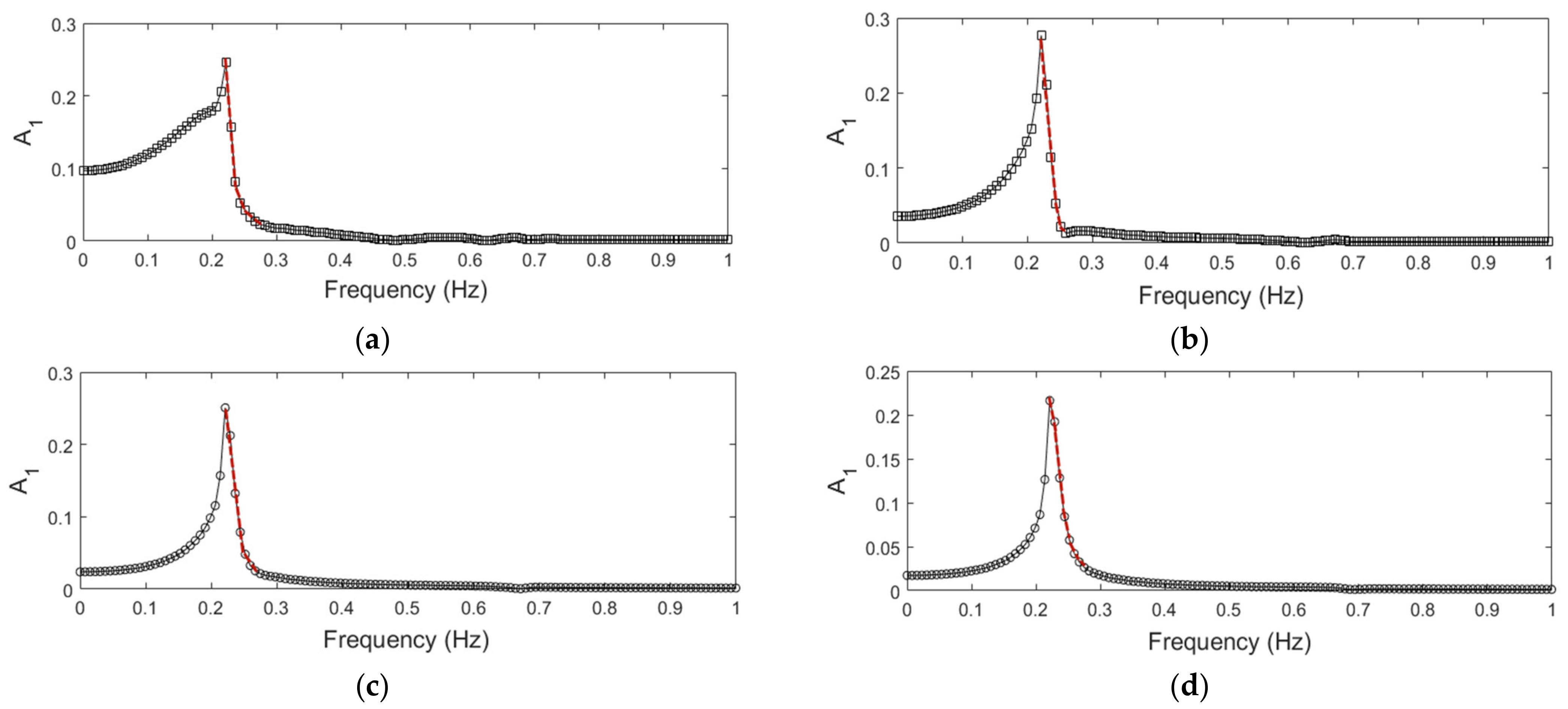
4.3. Numerical Simulations and Stability Analysis

Since multiple values appear in the steady-state solution, the stability of the steady-state solution should be investigated. The general approach of the CVHBM is employed here to judge the stability [29]. The response is rewritten in the form of:

$$\overline{z}=A_1(\tau )\cos (\Omega \tau +\phi (\tau ))$$

(50)

Substituting Equation (50) into (24), and then by using trigonometric transformation, equating the coefficients of equivalent first-order harmonics results in two coupled differential equations:

$${A_1}^{″}=-\left\{\begin{array}{l}\left[\frac{15}{32}-\frac{7}{2}{\sigma }_2{(\Omega +{\phi }^{\prime })}^2\right]A_1{}^5+\\ \left[3(\frac{1}{4}+{\sigma }_2)+5{\sigma }_2{(A_1{}^{\prime })}^2-4{\sigma }_2{(\Omega +{\phi }^{\prime })}^2\right]A_1{}^3\\ +\left[3{\sigma }_2{(A_1{}^{\prime })}^2+(8-4{\sigma }_1{(\Omega +{\phi }^{\prime })}^2)\right]A_1\\ +8\zeta A_1{}^{\prime }-4u_0{\Omega }^2\cos \phi \end{array}\right\}/(4{\sigma }_1+3{\sigma }_2{A}_1{}^2+\frac{5}{2}{\sigma }_2{A}_1{}^4)$$

(51)

$${\phi }^{″}=-\frac{(\Omega +{\phi }^{\prime })\left[(8{\sigma }_1+6{\sigma }_2{A}_1{}^2+5{\sigma }_2{A}_1{}^4)A_1{}^{\prime }+16\zeta A_1\right]+8u_0{\Omega }^2\sin \phi }{8{\sigma }_1{A}_1+2{\sigma }_2{A}_1{}^3+{\sigma }_2{A}_1{}^5}$$

(52)

Rewriting Equations (51) and (52) in the form of the equation of state, the Jacobian matrix can be calculated to be:

$$J=\left[\begin{array}{cccc}0& 0& 1& 0\\ 0& 0& 0& 1\\ J_{31}& -\frac{8u_0{\Omega }^{2}sin{x}_2}{5{\sigma }_2{x_1}^4+6{\sigma }_2{x_1}^2+8{\sigma }_1}& -\frac{4(5{\sigma }_2{x_1}^3{x}_3+3{\sigma }_2{x}_1{x}_3+4\zeta )}{5{\sigma }_2{x_1}^4+6{\sigma }_2{x_1}^2+8{\sigma }_1}& \frac{(\Omega +x_4)(14{\sigma }_2{x_1}^5+16{\sigma }_2{x_1}^3+16{\sigma }_1{x}_1)}{5{\sigma }_2{x_1}^4+6{\sigma }_2{x_1}^2+8{\sigma }_1}\\ J_{41}& -\frac{8u_0{\Omega }^{2}cos{x}_2}{8{\sigma }_1{x}_1+2{\sigma }_2{x_1}^3+{\sigma }_2{x_1}^5}& -\frac{(\Omega +x_4)(5{\sigma }_2{x_1}^4+6{\sigma }_2{x_1}^2+8{\sigma }_1)}{8{\sigma }_1{x}_1+2{\sigma }_2{x_1}^3+{\sigma }_2{x_1}^5}& -\frac{16\zeta x_1+x_3(5{\sigma }_2{x_1}^4+6{\sigma }_2{x_1}^2+8{\sigma }_1)}{8{\sigma }_1{x}_1+2{\sigma }_2{x_1}^3+{\sigma }_2{x_1}^5}\end{array}\right]$$

(53)

where $A_1\to x_1,\phi \to x_2,A_1{}^{\prime }\to x_3,{\phi }^{\prime }\to x_4$

$$\begin{array}{cc}\hfill & J_{31}=\frac{\left[35{\sigma }_2{(\Omega +x_4)}^2/2-75/32\right]{x_1}^4-3{x_1}^2\left[5{\sigma }_2{x_3}^2+3(1/4+{\sigma }_2)-4{\sigma }_2{(\Omega +x_4)}^2\right]-3{\sigma }_2{x_3}^2+4{\sigma }_1{(\Omega +x_4)}^2-8}{5{\sigma }_2{x_1}^4/2+3{\sigma }_2{x_1}^2+4{\sigma }_1}\hfill \\ \hfill & -\frac{10{\sigma }_2{x_1}^3+6{\sigma }_2{x}_1}{{(5{\sigma }_2{x_1}^4/2+3{\sigma }_2{x_1}^2+4{\sigma }_1)}^2}\left[(\frac{7}{2}{\sigma }_2{(\Omega +x_4)}^2-\frac{15}{32}){x_1}^5\right.+(4{\sigma }_2{(\Omega +x_4)}^2-5{\sigma }_2{x_3}^2-3(\frac{1}{4}+{\sigma }_2)){x_1}^3\hfill \\ \hfill & \left.-(3{\sigma }_2{x_3}^2+(8-4{\sigma }_1{(\Omega +x_4)}^2))x_1-8\zeta x_3+4u_0{\Omega }^{2}cos{x}_2\right]\hfill \end{array}$$

(54)

$$\begin{array}{l}{J}_{41}=-\frac{(\Omega +x_4)\left[12{\sigma }_2{x}_1{x}_3+20{\sigma }_2{x}_1{}^3{x}_3+16\zeta \right]}{8{\sigma }_1{x}_1+2{\sigma }_2{x}_1{}^3+{\sigma }_2{x}_1{}^5}+\\ \frac{(8{\sigma }_1+6{\sigma }_2{x}_1{}^2+5{\sigma }_2{x}_1{}^4)\left[(\Omega +x_4)((8{\sigma }_1+6{\sigma }_2{x}_1{}^2+5{\sigma }_2{x}_1{}^4)x_3+16\zeta x_1)+8u_0{\Omega }^2\sin x_2\right]}{{(8{\sigma }_1{x}_1+2{\sigma }_2{x}_1{}^3+{\sigma }_2{x}_1{}^5)}^2}\end{array}$$

(55)

By the eigenvalues of the Jacobian matrix, the stability of the steady-state response can be examined. When the system reaches the steady state, the Jacobian matrix can be described as a function of response amplitude and frequency as below. Thus, the stable and unstable regions in the amplitude-frequency plane can be obtained:

$$J(A_1,\Omega )=\left[\begin{array}{cc}{\mathrm{O}}_2& {\mathrm{E}}_2\\ \mathrm{R}(A_1,\Omega )& \mathrm{\Theta }(A_1,\Omega )\end{array}\right]$$

(56)

where ${\mathrm{O}}_2$ and ${\mathrm{E}}_2$ represent a second-order zero matrix and identity matrix, respectively. By transformation of Equations (51) and (52) and $x_3=x_4=0$, matrices $\mathrm{R}(A_1,\Omega )$ and $\mathrm{\Theta }(A_1,\Omega )$ are, respectively:

$$\mathrm{R}(A_1,\Omega )=\left[\begin{array}{cc}{\mathrm{R}}_{11}(A_1,\Omega )& \frac{16\zeta \Omega A_1}{5{\sigma }_2{x}_1{}^4+6{\sigma }_2{x}_1{}^2+8{\sigma }_1}\\ -\frac{16\zeta \Omega }{8{\sigma }_1{A}_1+2{\sigma }_2{A}_1{}^3+{\sigma }_2{A}_1{}^5}& {\mathrm{R}}_{22}(A_1,\Omega )\end{array}\right]$$

(57)

$$\mathrm{\Theta }(A_1,\Omega )=\left[\begin{array}{cc}-\frac{16\zeta }{5{\sigma }_2{A}_1{}^4+6{\sigma }_2{A}_1{}^2+8{\sigma }_1}& \frac{\Omega (14{\sigma }_2{A}_1{}^5+16{\sigma }_2{A}_1{}^3+16{\sigma }_1{A}_1)}{5{\sigma }_2{x}_1{}^4+6{\sigma }_2{x}_1{}^2+8{\sigma }_1}\\ -\frac{\Omega (5{\sigma }_2{A}_1{}^4+6{\sigma }_2{A}_1{}^2+8{\sigma }_1)}{8{\sigma }_1{A}_1+2{\sigma }_2{A}_1{}^3+{\sigma }_2{A}_1{}^5}& -\frac{16\zeta }{8{\sigma }_1+2{\sigma }_2{A}_1{}^2+{\sigma }_2{A}_1{}^4}\end{array}\right]$$

(58)

$${\mathrm{R}}_{11}(A_1,\Omega )=\frac{\left[35{\sigma }_2{\Omega }^2/2-75/32\right]A_1{}^4-3A_1{}^2\left[3(1/4+{\sigma }_2)-4{\sigma }_2{\Omega }^2\right]+4{\sigma }_1{\Omega }^2-8}{5{\sigma }_2{A}_1{}^4/2+3{\sigma }_2{A}_1{}^2+4{\sigma }_1}$$

(59)

$${\mathrm{R}}_{22}(A_1,\Omega )=-\frac{(15/16-7{\sigma }_2{\Omega }^2)A_1{}^5+6\left[3(\frac{1}{4}+{\sigma }_2)-4{\sigma }_2{\Omega }^2\right]A_1{}^3+2A_1(8-4{\sigma }_1{\Omega }^2)}{8{\sigma }_1{A}_1+2{\sigma }_2{A}_1{}^3+{\sigma }_2{A}_1{}^5}$$

(60)

To calculate the eigenvalues ${\lambda }_e$ of the Jacobian matrix $J$, the following equation is introduced:

$$\det \left(\left[\begin{array}{cc}{\lambda }_e{\mathrm{E}}_2-\mathrm{\Theta }& {\mathrm{E}}_2\\ {\mathrm{E}}_2& {\mathrm{O}}_2\end{array}\right]\right)=1$$

(61)

Then,

$$\det \left(\mathrm{J}-{\lambda }_e\mathrm{E}\right)=\det \left(\left[\begin{array}{cc}{\lambda }_e{\mathrm{E}}_2-\mathrm{\Theta }& {\mathrm{E}}_2\\ {\mathrm{E}}_2& {\mathrm{O}}_2\end{array}\right]\right)\cdot \det \left(\mathrm{J}-{\lambda }_e\mathrm{E}\right)=\det \left(\left[\begin{array}{cc}{\lambda }_e{\mathrm{E}}_2-\mathrm{\Theta }& {\mathrm{E}}_2\\ {\mathrm{E}}_2& {\mathrm{O}}_2\end{array}\right]\left[\begin{array}{cc}-{\lambda }_e{\mathrm{E}}_2& {\mathrm{E}}_2\\ \mathrm{R}& \mathrm{\Theta }-{\lambda }_e{\mathrm{E}}_2\end{array}\right]\right)=\det \left(\mathrm{R}+{\lambda }_e\mathrm{\Theta }-{\lambda }_e{}^2{\mathrm{E}}_2\right)$$

(62)

where $\mathrm{E}$ represents the fourth-order identity matrix. When $\det \left(\mathrm{R}+{\lambda }_e\mathrm{\Theta }-{\lambda }_e{}^2{\mathrm{E}}_2\right)=0$, the eigenvalues ${\lambda }_e$ can be obtained. If all real parts of eigenvalues are negative, the steady-state response of system has the stable solution, otherwise it has the unstable solution.

The dynamic Equation (25) is solved directly using the fourth order Runge–Kutta algorithm to observe the possible responses of the suspension system. In addition, the numerical simulation helps confirm the accuracy of the appropriate solutions obtained by the HBM. Figure 9 shows the calculated displacements in the harmonic response. In this system response, it can be found that the amplitude of displacement decreases as the excitation amplitude decreases, and the decline rate of their amplitude displacements basically become consistent. Figure 10 shows the frequency response curves under different excitation amplitudes and the red dotted lines of the FRCs represent the unstable regions. It can be seen that the amplitudes of displacement for the frequency response curves are varied under different excitation amplitudes and the corresponding peak frequency variation basically remains unchanged. When the excitation amplitude is larger than a certain value, there are three steady-state solutions occurring at the same frequency, two of which are stable and one unstable.

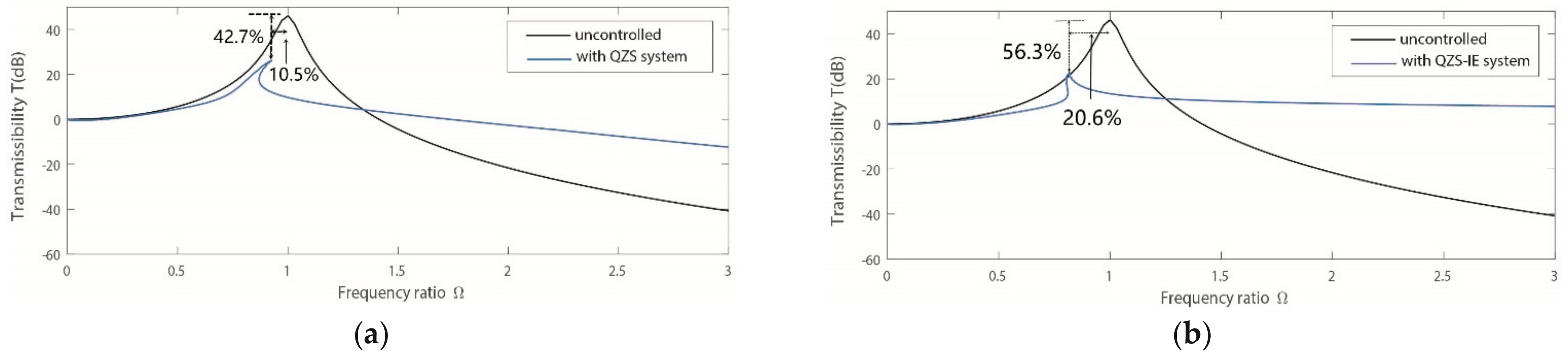
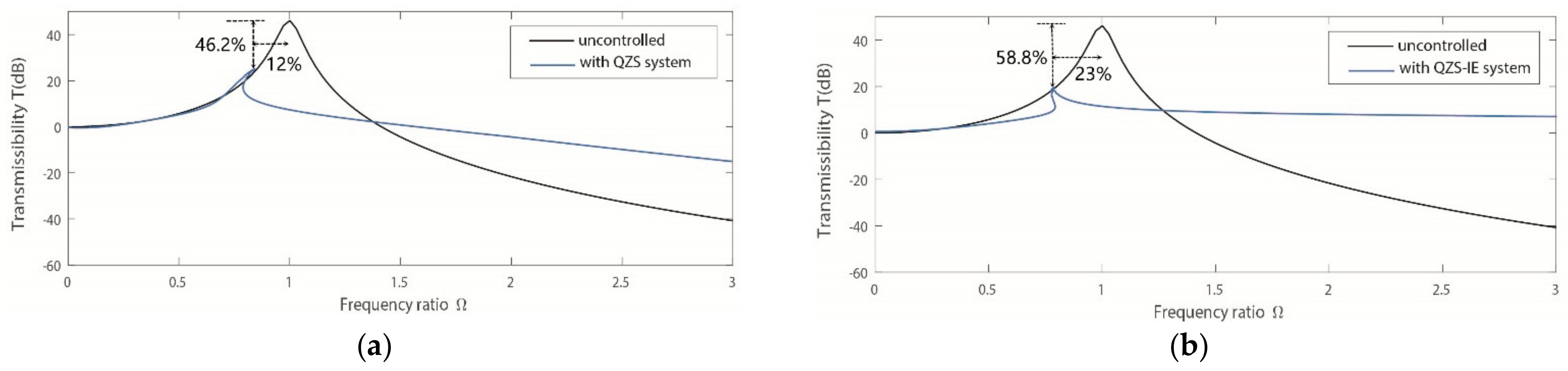
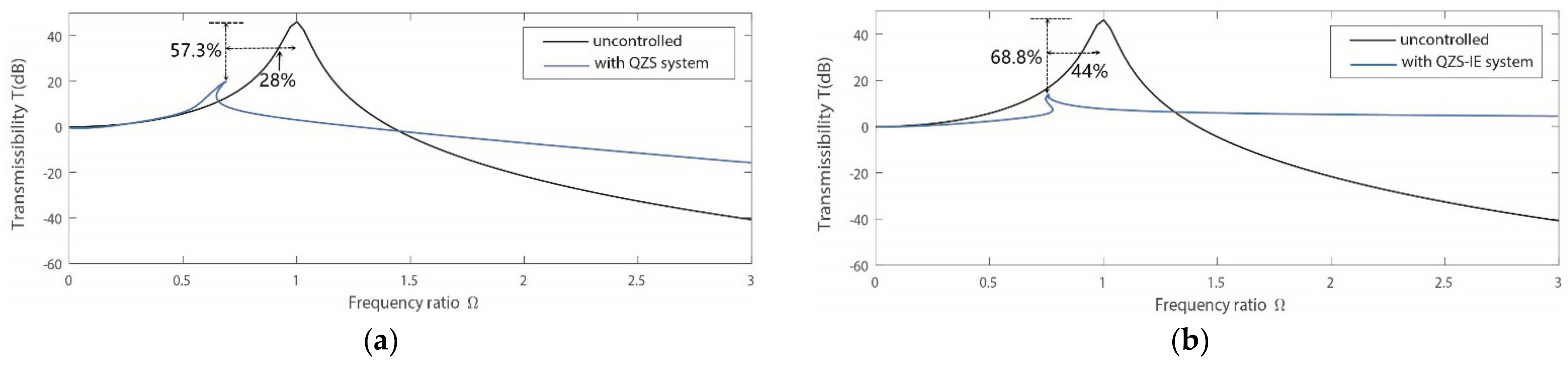
5. Vibration Suppression Effect

The vibration suppression effects of the seat suspension system are investigated in this section. The maximum absolute displacement transmissibility for the uncontrolled system ($\zeta =0.05$) and the controlled system is denoted as $T_{uc}$ and $T_c$, respectively. The reduction percentage of the maximum absolute displacement transmissibility for the controlled system is:

$$Q_T=\frac{T_{uc}-T_c}{T_{uc}}100\%$$

(63)

The frequency ratio at the maximum resonance response peak for the uncontrolled system ($\zeta =0.05$) and the controlled system is denoted as ${\Omega }_{uc}$ and ${\Omega }_c$, respectively. The reduction percentage of the frequency at the maximum resonance response peak for the controlled system is:

$$Q_{\Omega }=\frac{{\Omega }_{uc}-{\Omega }_c}{{\Omega }_{uc}}100\%$$

(64)

Figure 11 shows the comparisons of the vibration suppression effects between the QZS system without inerter element and the QZS-IE system when the excitation amplitude is $u_0=1.0$. It can be observed that the frequency response curves of both systems have obvious nonlinear characteristics, especially at the maximum resonance response peak. The vibration suppression effect can be severely affected by the strong nonlinear characteristics. As shown in Figure 11a, for the quasi-zero-stiffness system, the reduction percentage of the maximum displacement transmissibility is 42.7%. The reduction percentage of the frequency at the maximum resonance peak is only 10.5%. However, for the QZS-IE system, Figure 11b shows that the reduction percentages of the maximum displacement transmissibility and frequency at the maximum resonance peak are, respectively, 56.3% and 20.6%. Obviously, it is concluded that the QZS-IE system has significant vibration suppression advantages for the maximum resonance response peak. In addition, in the high frequency region, the curves of the QZS system, the QZS-IE system, and the uncontrolled system are not coincident. The vibration suppression effect of the displacement transmissibility of the QZS-IE system is slightly worse, especially for a frequency ratio greater than 1.25; the displacement transmissibility of the QZS-IE system is slightly higher than that of the QZS system and the uncontrolled system.

Next, the influence of the excitation amplitude on the vibration suppression effect is analyzed. When $u_0=0.9$ and $u_0=0.4$, the comparisons of the vibration suppression effects between the QZS system and the QZS-IE system are shown in Figure 12 and Figure 13, respectively. It can be found that with a decrease in excitation amplitude, the curve changes of the two systems have the same trend when the frequency ratio is about larger than 0.9. Moreover, the value of $Q_T$ and $Q_{\Omega }$ for both systems increases as the excitation amplitude decreases. For the QZS system, the displacement transmissibility curve bends to the right, which reduces the effective isolation region. In contrast, for the QZS-IE system, the bending trend of the displacement transmissibility curve is considerably weakened, thereby, resulting in a much wider isolation frequency range as well as a lower peak transmissibility.

Meanwhile, with a decrease in the excitation amplitude, the differences of $Q_T$ between the QZS-IE system and the QZS system are, respectively, 13.6%, 12.6%, and 11.5%, and the differences of $Q_{\Omega }$ are 9.5%, 11%, and 16%, respectively. Therefore, this illustrates that for the maximum displacement transmissibility, the larger the excitation amplitude is, the greater the advantage of the QZS-IE system in vibration suppression performance. For the frequency at the maximum resonance response peak, although the difference value variation is the opposite, the changing gradient gradually decreases and the vibration suppression performance is not seriously affected. The QZS-IE system still has better performance advantages.

6. Parameter Studies and Discussions

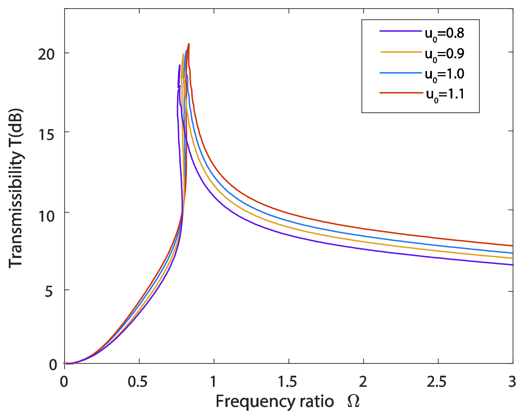
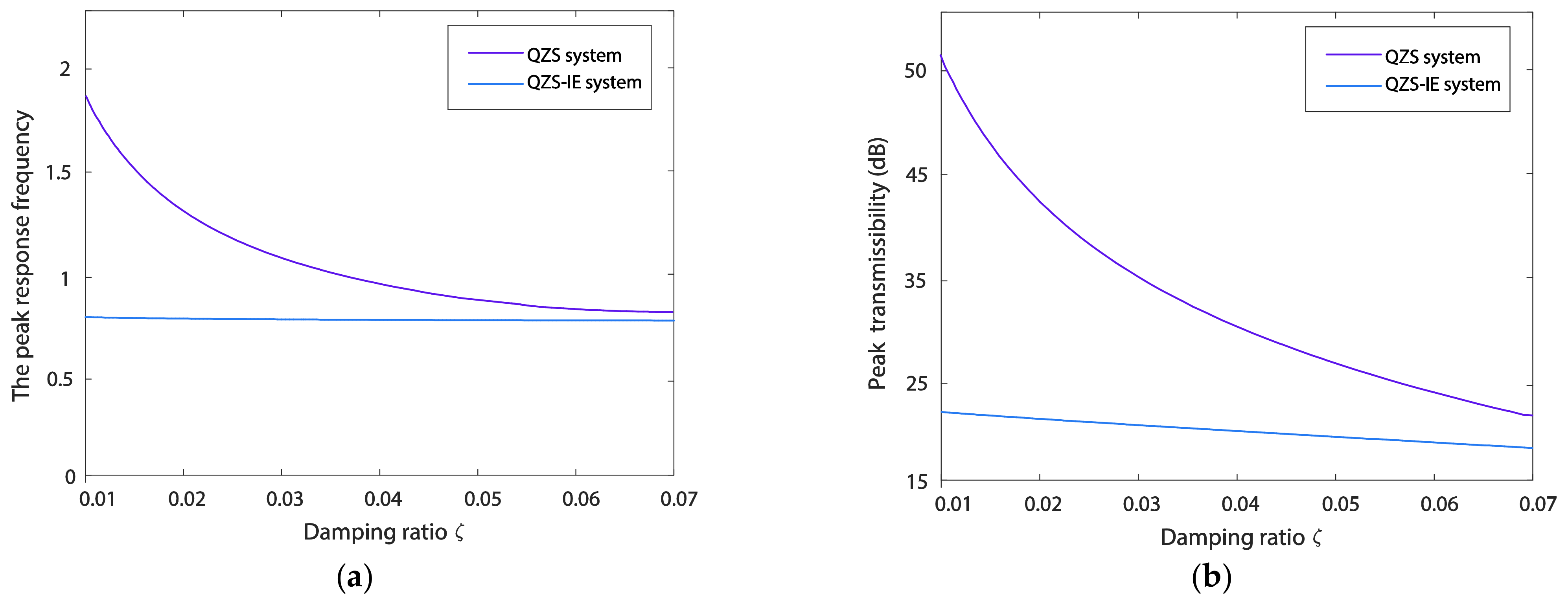
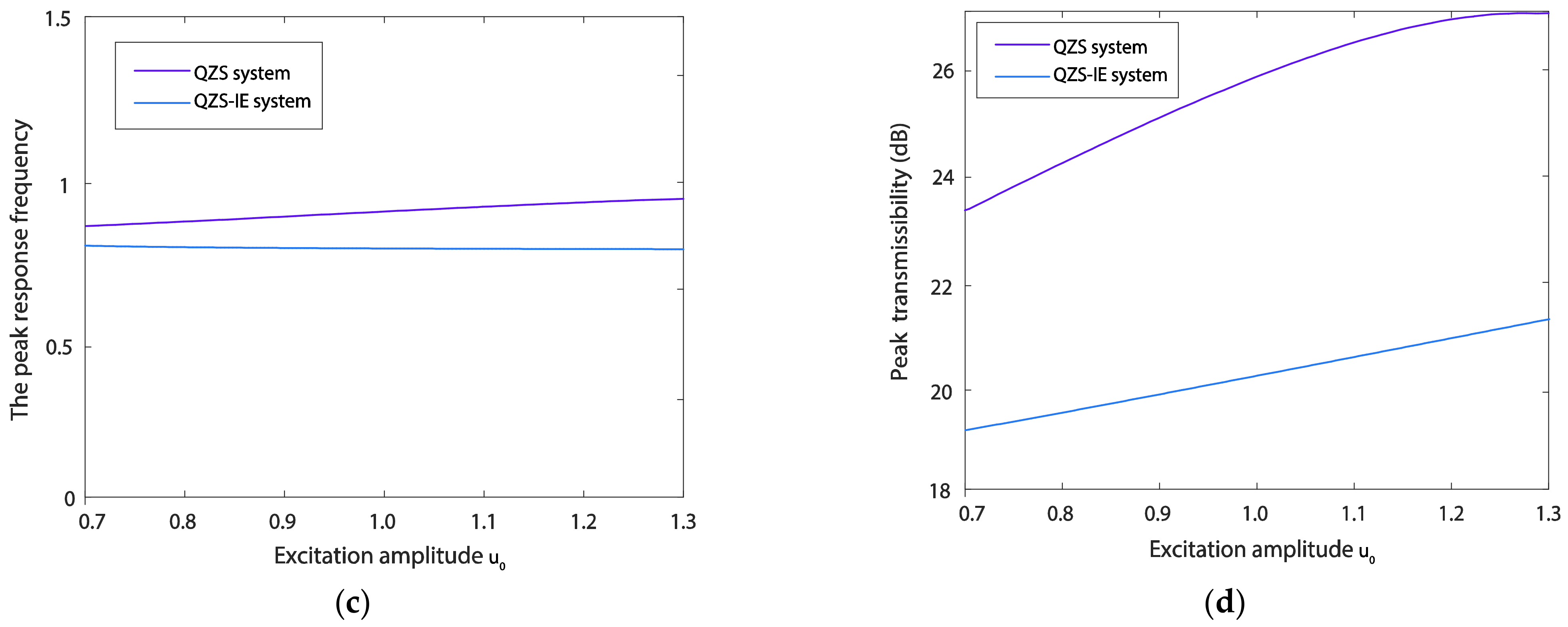
6.1. Influences of Excitation Amplitude and Damping Ratio on the Transmissibility

For a QZS isolator with hardening stiffness, the frequency response curve can have a potential trend of bending to the right, which leads to a jump phenomenon in the response amplitude and transmissibility. In the jump frequency range, there exist three possible solutions, namely three values of transmissibility. The intermediate branch of FRCs has been proved unstable in Section 4.3. Therefore, the vibration isolation effect in the jump frequency ranges may be unstable, and the isolation frequency and peak transmissibility (the maximum value of the transmissibility) are two important indexes to be considered for a nonlinear suspension system with hardening stiffness. In the following section, the influences of the excitation amplitude and damping on the transmissibility and isolation frequency are discussed.

The absolute displacement transmissibility of the QZS-IE system under different excitation amplitudes is shown in Figure 14. The maximum amplitude of transmissibility increases extremely slowly as the excitation amplitude increases. The same case is also found in Figure 15 and the maximum amplitude of transmissibility decreases slowly as the frequency ratio increases. Thus, it can be observed that the QZS-IE system is insensitive to the variations of excitation amplitude and frequency ratio under large excitation and small damping. This insensitivity causes the isolation frequency and peak transmissibility of the QZS-IE system to remain at a lower level than those of the QZS system. In addition, the peaks of the frequency response curve and the transmissibility curve look very “sharp” under large excitation and small damping, so it can be concluded that the transmissibility reaches the maximum when the peak response occurs. Therefore, the frequency corresponding to the maximum value of transmissibility is considered to be the isolation frequency, and the calculation of isolation frequencies converted into the calculation of peak response frequency.

Figure 16a,b shows the variation trends of peak response frequency and peak transmissibility of the QZS-IE system and the QZS system with varying damping ratio, and Figure 16c,d shows those with varying excitation amplitude. It can be seen that increasing the damping ratio or decreasing the excitation amplitude causes a relatively noticeable decrease in the peak response frequency and peak transmissibility for the QZS system without inerter element, except that the peak response frequency varies less when increasing the excitation amplitude. Whereas for the QZS-IE system, the peak response frequency and peak transmissibility seem to remain unchanged or vary a little when varying the damping ratio and excitation amplitude; only the peak transmissibility is increased when the damping ratio decreases. As a result, it can be concluded that the peak response frequency and peak transmissibility of the QZS-IE system are much lower than those of the QZS system, especially when under large excitation and small damping.

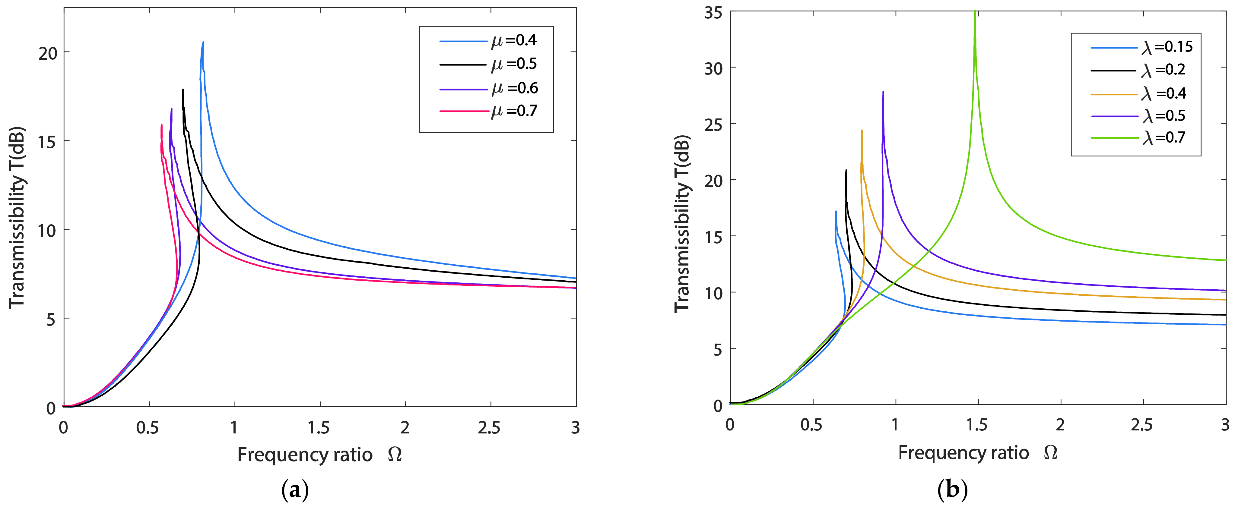
6.2. Influences of Parameter Selection for the Inerter Element on the Transmissibility

The parameters of additional tunable inerter element are related to the mass and location of the inerter element. In this section, the influences of the parameters $\mu$ and $\lambda$ on the vibration isolation performance are investigated in detail. Figure 17 shows the absolute displacement transmissibility curves under different parameters $\mu$ and $\lambda$. As the mass ratio increases, the peak of the transmissibility curve decreases gradually, and the transmissibility curve leans to the left. This will undoubtedly lead to a lower transmissibility and a wider vibration isolation region. It can also be seen that a larger mass ratio contributes to the better vibration isolation performance. Therefore, the selection of mass ratio should be conducted according to a practical engineering application, on the premise that it is better to choose a larger mass ratio in a reasonable range. Moreover, it can be seen that the parameter $\lambda$ has an influence on vibration isolation performance in the low-frequency and high-frequency range. With the increasing of $\lambda$, the peak response frequency and peak transmissibility have both increased. Nevertheless, if the value of the parameter $\lambda$ becomes much larger, it leads to an increase in the total mass on the one-side and larger static displacement. As a result, a relatively smaller value of parameter $\lambda$ can be better for vibration isolation performance of the QZS-IE seat suspension system.

7. Conclusions

In the presented study, a cab seat suspension system based on a NSS is designed and quasi-zero-stiffness conditions are put forward. The different structural parameters of the system and their influences on the dynamic stiffness characteristics are analyzed. The ideal configuration parameter range and final value of the suspension system are obtained.

In this study, for a seat suspension structure of a construction machinery cab, the nonlinear dynamic model is established. The absolute displacement transmissibility of the QZS-IE system and the primary response and the stability are analyzed by using HBM. Meanwhile, the numerical simulations by the fourth order Runge–Kutta method are conducted, which also verifies the agreement of the results of both methods.

By comparing with the quasi-zero-stiffness system, the vibration suppression effects of the QZS-IE system and parameter studies are presented. The results indicate that the QZS-IE system has higher vibration suppression efficiency under large excitation and small damping and lower transmissibility and a wider vibration isolation frequency range. For the QZS-IE system, the isolation frequency and peak transmissibility are kept at a lower level than those of the QZS system. The peak transmissibility can be increased by decreasing damping or increasing excitation amplitude, but the increasing rate is still much lower. Moreover, the parameter analysis of the inerter element shows that an inerter element with a larger mass ratio and a relatively shorter distance ratio is better for vibration isolation performance of the QZS-IE system in a practical engineering application.

References

1. Nguyen, S.D.; Nguyen, Q.H.; Choi, S.-B. A hybrid clustering based fuzzy structure for vibration control—Part 2: An application to semi-active vehicle seat-suspension system. Mech. Syst. Signal Process. 2015, 56–57, 288–301. [Google Scholar] [CrossRef]
2. Kulkarni, S.; Spencer, S.; Horton, D.J. Isolation Mount Assembly. U.S. Patent 11,001,306, 11 May 2021. [Google Scholar]
3. Deshmukh, S.R.; Krishnan Balaji, N.S.; Saharabhudhe, S.; Khubalkar, S.; Parameswaran, A.P. Designing of Control Strategy for High Voltage Battery Isolation in an Electric Vehicles. In Proceedings of the 2019 IEEE 5th International Conference for Convergence in Technology (I2CT), Bombay, India, 29–31 March 2019. [Google Scholar]
4. Zhentong, L.; Hongwen, H. Sensor fault detection and isolation for a lithium-ion battery pack in electric vehicles using adaptive extended Kalman filter. Appl. Energy 2017, 185, 2033–2044. [Google Scholar]
5. Griffin, M.J. Handbook of Human Vibration, 1st ed.; Academic Press: Cambridge, UK, 2012. [Google Scholar]
6. Friesenbichler, B.; Nigg, B.M.; Dunn, J.F. Local metabolic rate during whole body vibration. J. Appl. Physiol. 2013, 114, 1421–1425. [Google Scholar] [CrossRef] [PubMed] [Green Version]
7. Carletti, E.; Pedrielli, F. Tri-axial evaluation of the vibration transmitted to the operators of crawler compact loaders. Int. J. Ind. Ergon. 2018, 68, 46–56. [Google Scholar] [CrossRef]
8. ISO. Mechanical Vibration and Shock: Evaluation of Human Exposure to Whole-Body Vibration. Part 1, General Requirements: International Standard ISO 2631-1: 1997 (E); ISO: Geneva, Switzerland, 1997. [Google Scholar]
9. Knothe, K.; Stichel, S. (Eds.) Human perception of vibrations-ride comfort. In Rail Vehicle Dynamics; Springer: New York, NY, USA, 2017; pp. 141–157. [Google Scholar]
10. Van Eijk, J.; Dijksman, J. Plate spring mechanism with constant negative stiffness. Mech. Mach. Theory 1979, 14, 1–9. [Google Scholar] [CrossRef]
11. Lee, C.M.; Goverdovskiy, V.N.; Temnikov, A.I. Design of springs with “negative’’ stiffness to improve vehicle driver vibration isolation. J. Sound Vib. 2007, 302, 865–874. [Google Scholar] [CrossRef]
12. Yang, J.; Xiong, Y.; Xing, J. Dynamics and power flow behaviour of a nonlinear vibration isolation system with a negative stiffness mechanism. J. Sound Vib. 2013, 332, 167–183. [Google Scholar] [CrossRef]
13. Junshu, H.; Lingshuai, M.; Jinggong, S. Design and Characteristics Analysis of a Nonlinear Isolator Using a Curved-Mount-Spring-Roller Mechanism as Negative Stiffness Element. Math. Probl. Eng. 2018, 2018, 1–15. [Google Scholar] [CrossRef]
14. Yuanqing, F.; Peimin, G. A vibration Isolation Device for Elastic Elements in Parallel of Positive and Negative Stiffness. 1 November 1985. Available online: https://d.wanfangdata.com.cn/patent/CN85109107 (accessed on 25 July 2021).
15. Jianzhuo, Z.; Dan, L.; Shen, D.; Dong, S. A Study on Ultra-low Frequency Nonlinear Parallel Vibration Isolation System for Precision Instruments. China Mech. Eng. 2004, 15, 69–71. [Google Scholar]
16. Han, J.; Shishu, X.; Yong, Y. Analysis of structural vibration isolation effect based on negative stiffness principle. J. Huazhong Univ. Sci. Technol. 2010, 38, 76–79. [Google Scholar]
17. Donghai, L.; Shougen, Z.; Yujin, H.; Li, T. Dynamic analysis of quasi-zero stiffness isolator with time delay control. Vib. Shock. 2018, 37, 49–55. [Google Scholar]
18. Lu, Z.; Brennan, M.J.; Chen, L.-Q. On the transmissibilities of nonlinear vibration isolation system. J. Sound Vib. 2016, 375, 28–37. [Google Scholar] [CrossRef]
19. Sarlis, A.A.; Pasala, D.T.R.; Constantinou, M.C.; Reinhorn, A.M.; Nagarajaiah, S.; Taylor, D.P. Negative Stiffness Device for Seismic Protection of Structures. J. Struct. Eng. 2013, 139, 1124–1133. [Google Scholar] [CrossRef] [Green Version]
20. Palomares, E.; Nieto, A.; Morales, A.L.; Chicharro, J.; Pintado, P. Numerical and experimental analysis of a vibration isolator equipped with a negative stiffness system. J. Sound Vib. 2018, 414, 31–42. [Google Scholar] [CrossRef]
21. Davoodi, E.; Safarpour, P.; Pourgholi, M.; Khazaee, M. Design and evaluation of vibration reducing seat suspension based on negative stiffness structure. Proc. Inst. Mech. Eng. Part C J. Mech. Eng. Sci. 2020, 234, 4171–4189. [Google Scholar] [CrossRef]
22. Dong, G.; Zhang, X.; Xie, S.; Yan, B.; Luo, Y. Simulated and experimental studies on a high-static-low-dynamic stiffness isolator using magnetic negative stiffness spring. Mech. Syst. Signal Process. 2017, 86, 188–203. [Google Scholar] [CrossRef]
23. Yao, H.; Chen, Z.; Wen, B. Dynamic vibration absorber with negative stiffness for rotor system. Shock. Vib. 2016, 2016, 5231704. [Google Scholar] [CrossRef]
24. Liu, D.; Liu, Y.; Sheng, D.; Liao, W. Seismic response analysis of an isolated structure with QZS under near-fault vertical earthquakes. Shock. Vib. 2018, 10, 1–12. [Google Scholar] [CrossRef] [Green Version]
25. Sun, X.; Jing, X. Multi-direction vibration isolation with quasi-zero stiffness by employing geometrical nonlinearity. Mech. Syst. Signal Process. 2015, 62, 149–163. [Google Scholar] [CrossRef]
26. Meng, Q.; Yang, X.; Li, W.; Lu, E.; Sheng, L. Research and analysis of quasi-zero-stiffness isolator with geometric nonlinear damping. Shock Vib. 2017, 9, 1–9. [Google Scholar] [CrossRef] [Green Version]
27. Zhao, F.; Ji, J.; Ye, K.; Luo, Q. An innovative quasi-zero stiffness isolator with three pairs of oblique springs. Int. J. Mech. Sci. 2021, 192, 106093. [Google Scholar] [CrossRef]
28. Sun, X.; Zhang, J. Displacement transmissibility characteristics of harmonically base excited damper isolators with mixed viscous damping. Shock. Vib. 2013, 20, 921–931. [Google Scholar] [CrossRef]
29. Liu, C.; Yu, K. A high-static–low-dynamic-stiffness vibration isolator with the auxiliary system. Nonlinear Dyn. 2018, 94, 1549–1567. [Google Scholar] [CrossRef]
Figure 1. Simplified model of the vehicle seat.
Applsci 11 06928 g001
Figure 2. Mathematical model of the seat isolation system with inerter elements.
Applsci 11 06928 g002
Figure 3. Dimensionless force–deflection curves with various values of α ( γ 1 = 0.8 , γ 2 = 1.2 , η = 0.2 ).
Applsci 11 06928 g003
Figure 4. Dimensionless force–deflection curves with the various values of γ 1 : (a) α = 0.8, γ 2 = 1.2; (b) α = 1.0, γ 2 = 1.2; (c) α = 1.2, γ 2 = 1.2.
Applsci 11 06928 g004
Figure 5. Dimensionless force–deflection curves with the various values of γ 2 : (a) α = 0.8, γ 1 = 0.8; (b) α = 1.0, γ 1 = 0.8; (c) α = 1.2, γ 1 = 0.8.
Applsci 11 06928 g005
Figure 6. Dynamic stiffness curves of systems with the various values of γ 1 : (a) α = 0.6, γ 2 = 0.8; (b) α = 1.0, γ 2 = 0.8; (c) α = 1.2, γ 2 = 0.8.
Applsci 11 06928 g006
Figure 7. Dynamic stiffness curves of systems with the various values of γ 2 (z = H x ): (a) α = 0.5, γ 1 = 0.8; (b) α = 0.8, γ 1 = 0.8; (c) α = 1, γ 1 = 0.8; (d) α = 1.2, γ 1 = 0.8.
Applsci 11 06928 g007
Figure 8. Dynamic stiffness curves of systems with the various values of α (z = H x ).
Applsci 11 06928 g008
Figure 9. Displacement time histories.
Applsci 11 06928 g009
Figure 10. Frequency response curves under different excitation amplitudes ( μ = 0.4 , λ = 0.2 , ζ = 0.05 , ε = 2 ): (a) u 0 Ω 2 = 880 ; (b) u 0 Ω 2 = 870 ; (c) u 0 Ω 2 = 860 ; (d) u 0 Ω 2 = 820 .
Applsci 11 06928 g010
Figure 11. The vibration suppression effects of the seat suspension system ( u 0 = 1.0 ): (a) The displacement transmissibility of the QZS system without inerter elements; (b) the displacement transmissibility of the QZS-IE system.
Applsci 11 06928 g011
Figure 12. The vibration suppression effects of the seat suspension system ( u 0 = 0.9 ): (a) The displacement transmissibility of the QZS system without inerter elements; (b) the displacement transmissibility of the QZS-IE system.
Applsci 11 06928 g012
Figure 13. The vibration suppression effects of the seat suspension system ( u 0 = 0.4 ): (a) The displacement transmissibility of the QZS system without inerter elements; (b) the displacement transmissibility of the QZS-IE system.
Applsci 11 06928 g013
Figure 14. The absolute displacement transmissibility of the QZS-IE seat suspension system with different excitation amplitudes ( μ = 0.4 , λ = 0.2 , ζ = 0.05 , ε = 2 ).
Applsci 11 06928 g014
Figure 15. The absolute displacement transmissibility of the QZS-IE seat suspension system with different damping ratios ( μ = 0.4 , λ = 0.2 , u 0 = 1.0 , ε = 2 ).
Applsci 11 06928 g015
Figure 16. Comparisons of peak transmissibility and the peak response frequency between the QZS system and QZS-IE system ( λ = 0.2 , ε = 2 ): (a) The variation of peak response frequency with damping ratio ( u 0 = 1.0 ); (b) the variation of peak transmissibility with damping ratio ( u 0 = 1.0 ); (c) the variation of peak response frequency with excitation amplitude ( ζ = 0.05 ); (d) the variation of peak transmissibility with excitation amplitude ( ζ = 0.05 ).
Applsci 11 06928 g016aApplsci 11 06928 g016b
Figure 17. The absolute displacement transmissibility of the QZS-IE seat suspension system with different parameters of the inerter element: (a) Variation of μ at ζ = 0.05 ,   λ = 0.2 ,   u 0 = 1.0 ,   ε = 2 ; (b) variation of λ at ζ = 0.05 ,   μ = 0.4 ,   u 0 = 1.0 ,   ε = 2 .
Applsci 11 06928 g017
Publisher’s Note: MDPI stays neutral with regard to jurisdictional claims in published maps and institutional affiliations.