
Investigation of Pressure Oscillation and Cavitation Characteristics for Submerged Self-Resonating Waterjet

Abstract
:1. Introduction
2. Multi-Fluid Model and Numerical Method
2.1. Governing Equations
2.2. Turbulence Model
2.3. Schnerr-Sauer Cavitation Model (SS)
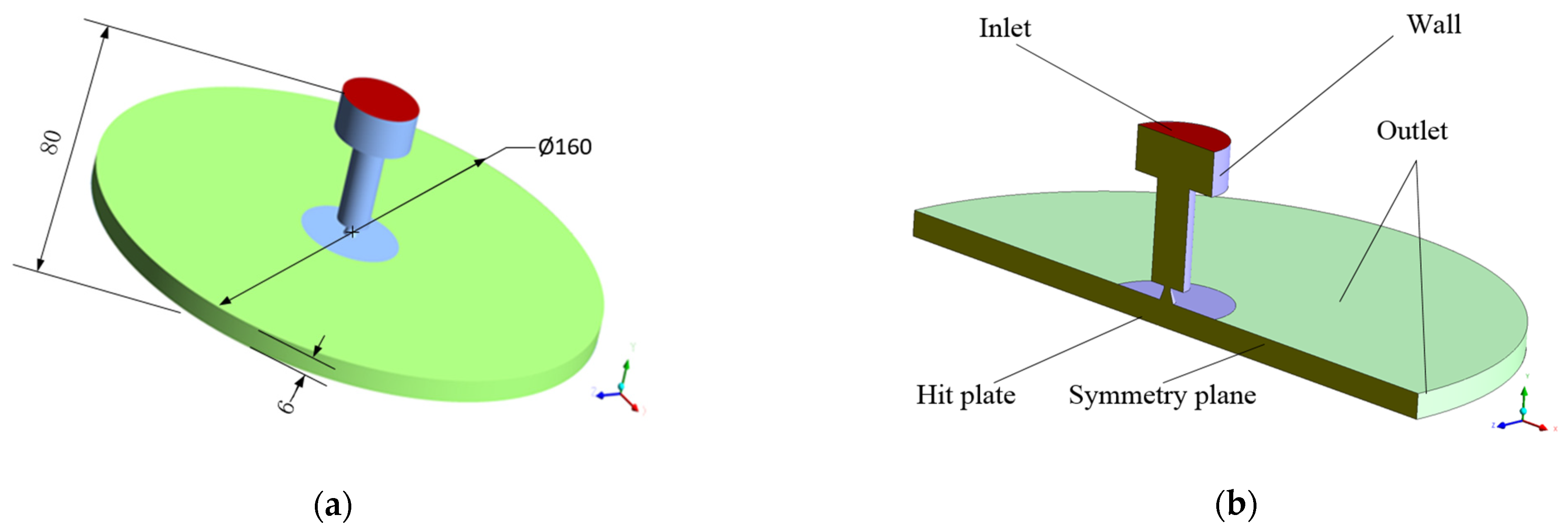
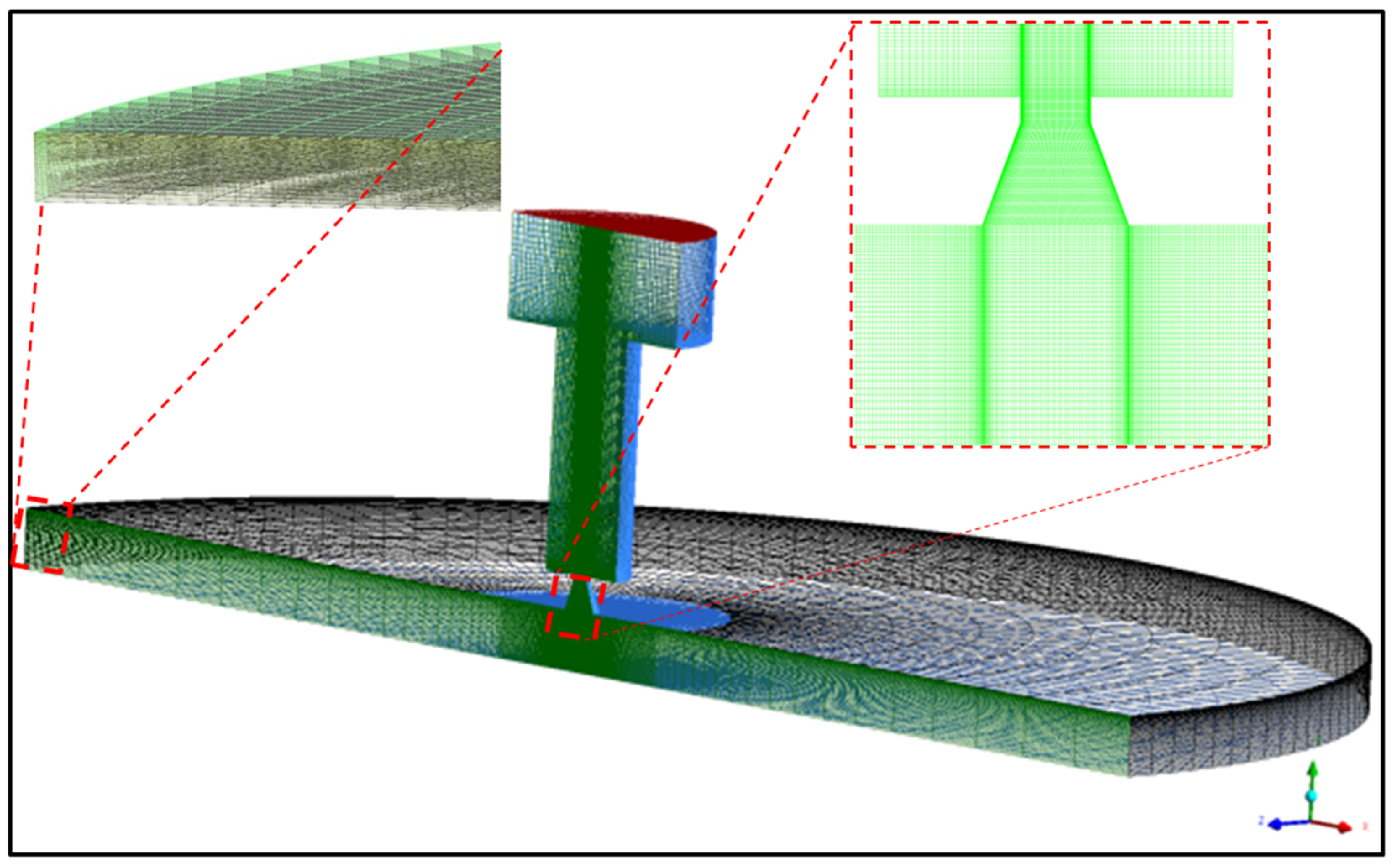
2.4. Numerical Setup
3. Experimental Test and Validation
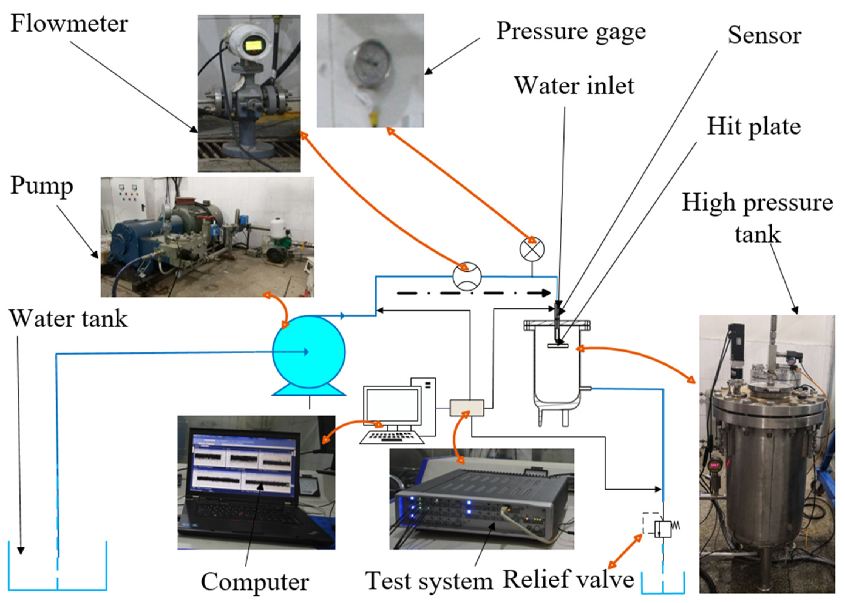
3.1. Experimental Setup
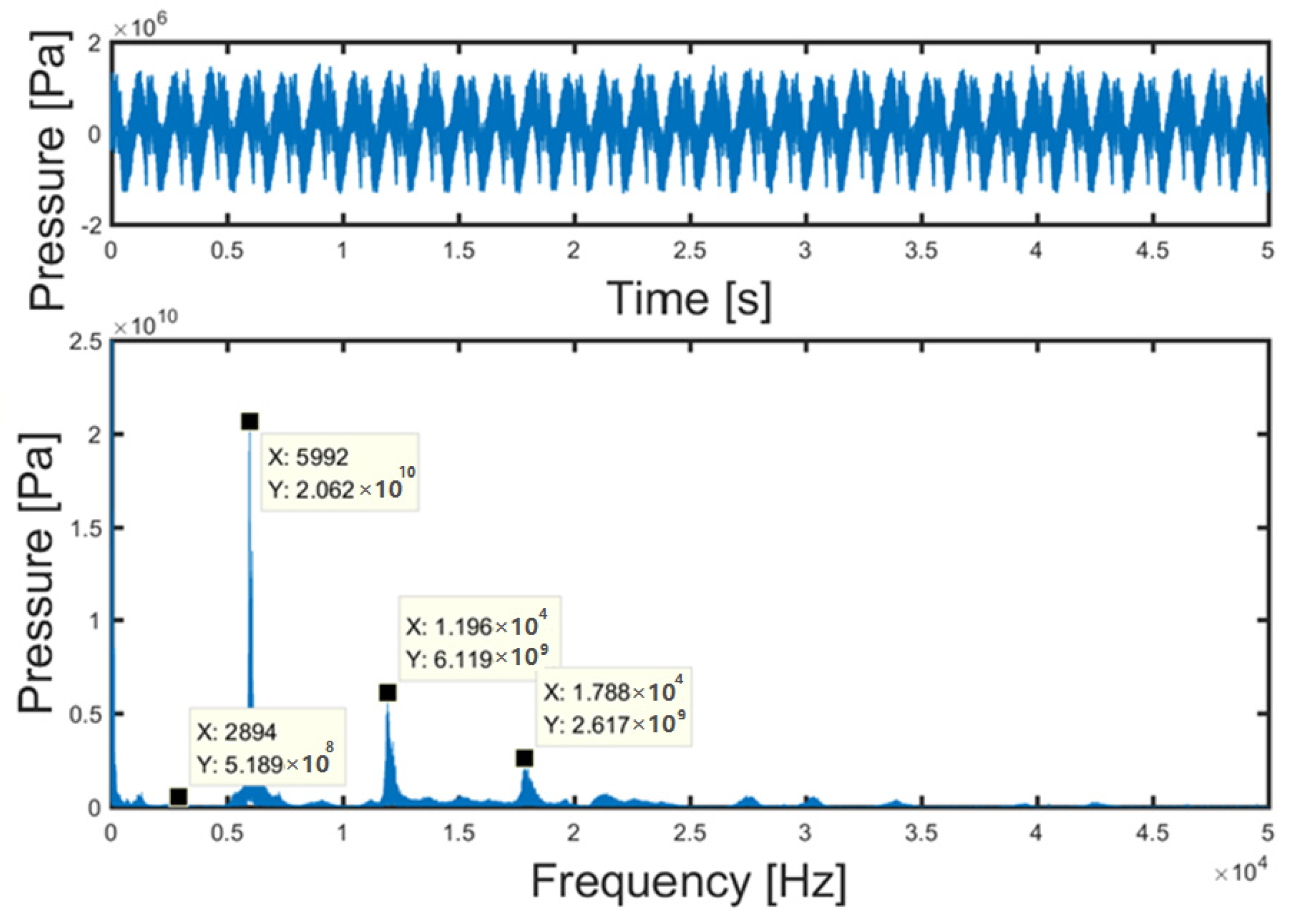
3.2. Validation
4. Simulations Results and Discussions
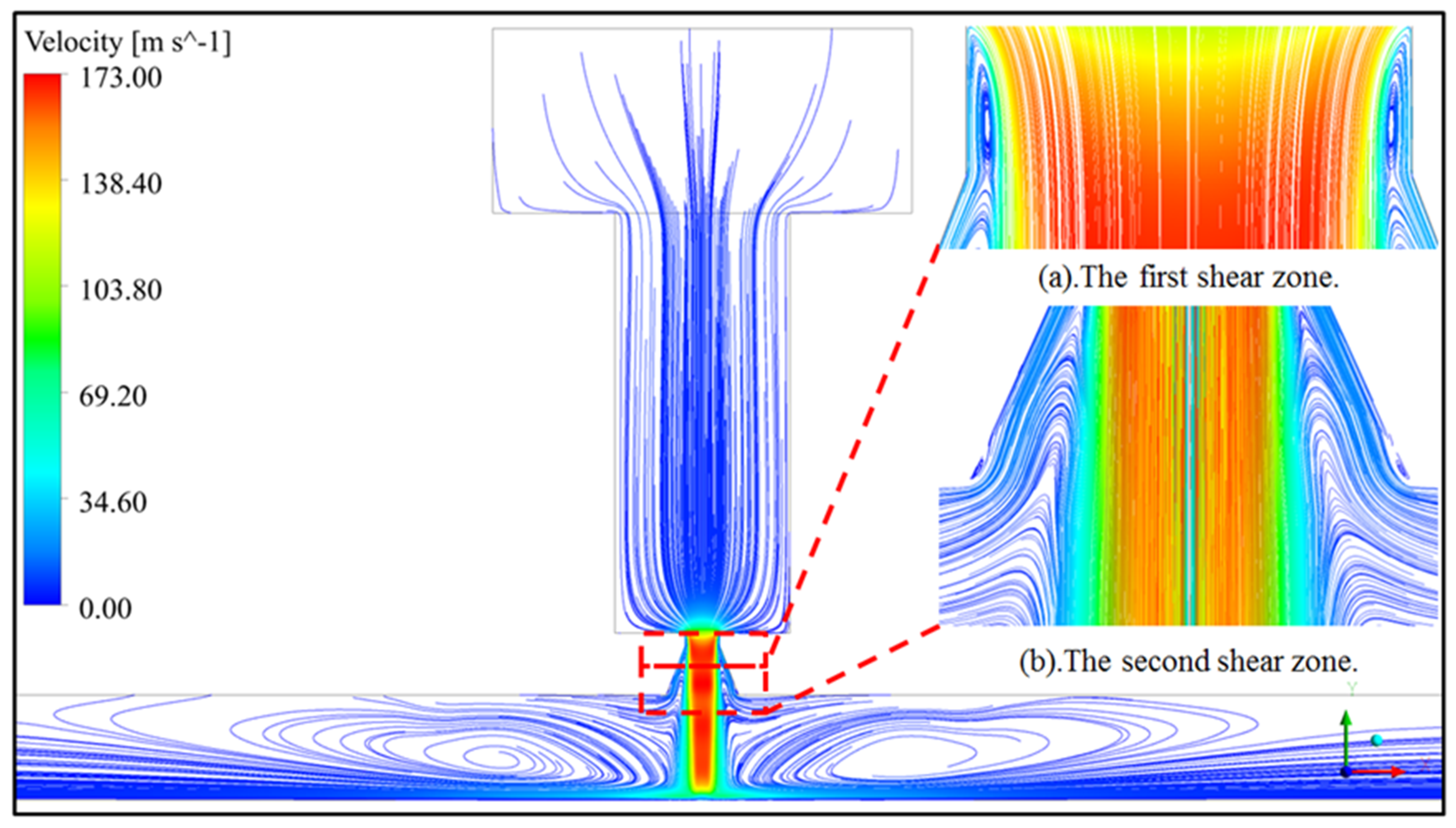
4.1. Velocity Distribution
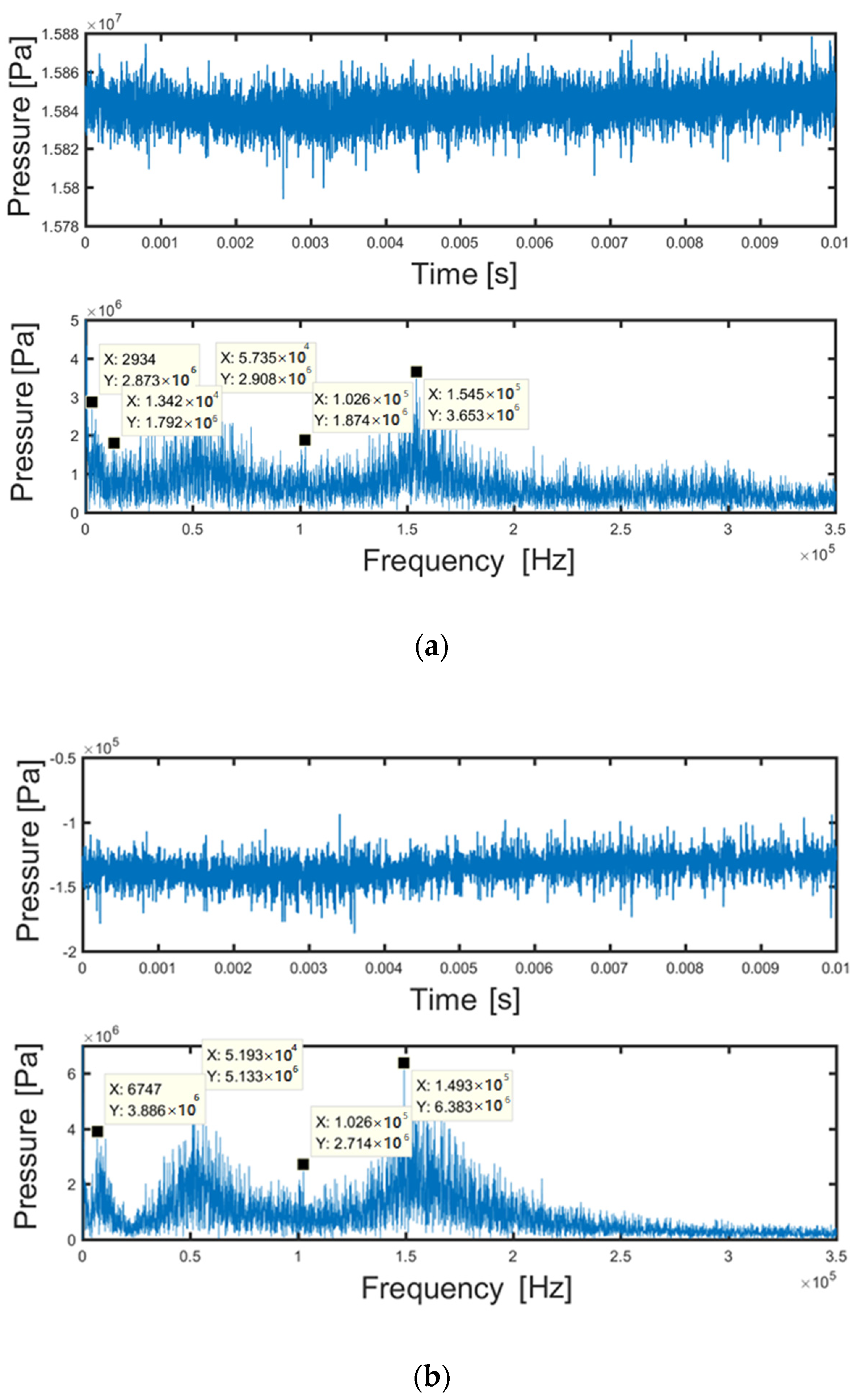
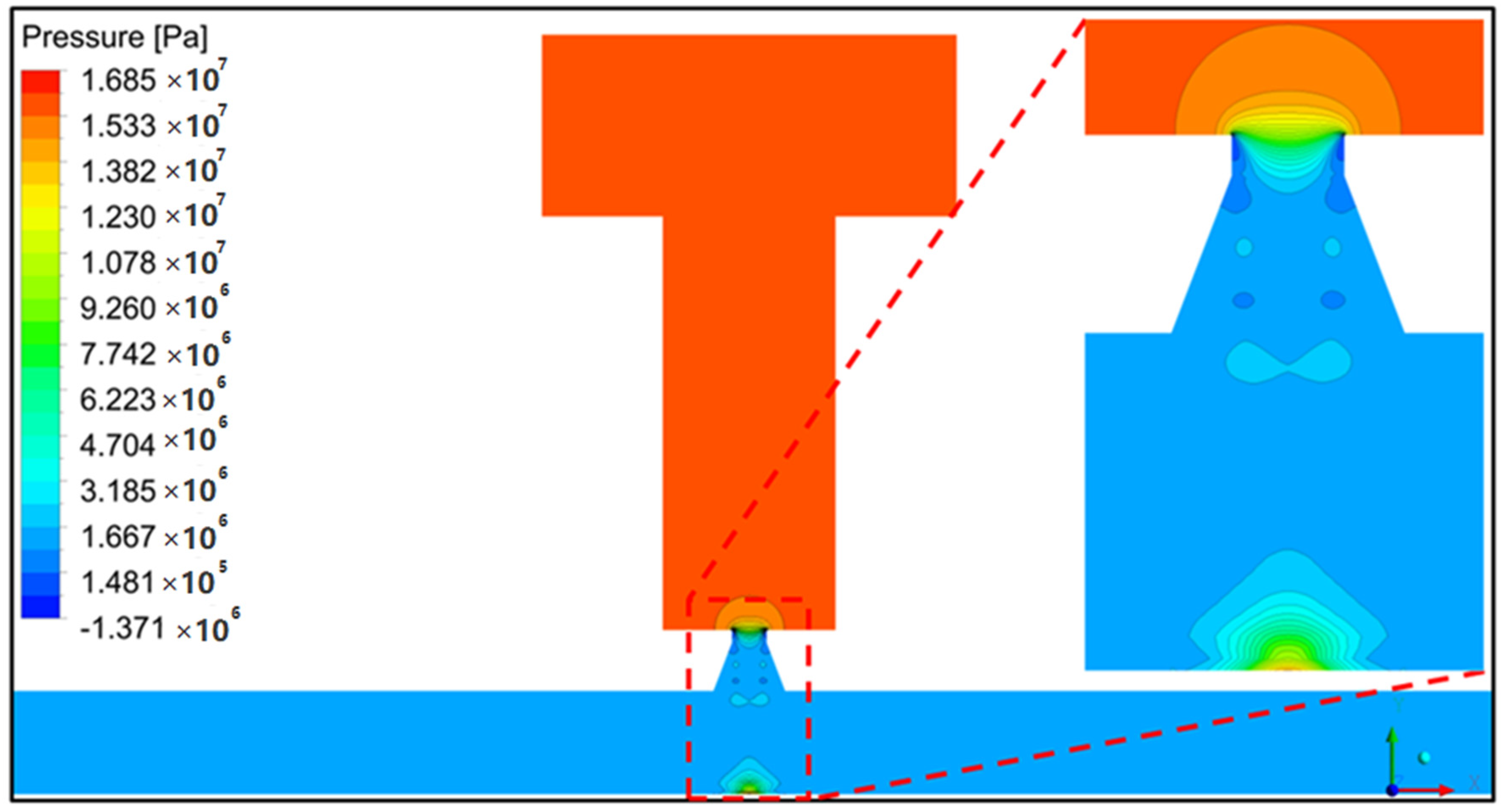
4.2. Pressure Oscillation Characteristics
4.3. Cavitation Characteristics
5. Conclusions
- (1)
- The sudden change of the flow velocity for the geometry of the nozzle formation the velocity vortexes consists of two shear zones. The first shear zone is the formation by the interaction between the shear layer of the jet and the inner surface of the nozzle; the second shear zone is because of the high-speed jet inflow into the relatively stationary liquid, and the strength of the vortex is much lower than the first shear zone.
- (2)
- Velocity vector backwash produces a low-pressure region, and at the strongest position of our research, the negative pressures inside the conduits can drop down to −1.3 MPa. At the same time, the distribution of the bubbles along with the jet shedding from the throat of the nozzle periodic, the cavitation depends on the relation between the pressure and the vapor pressure.
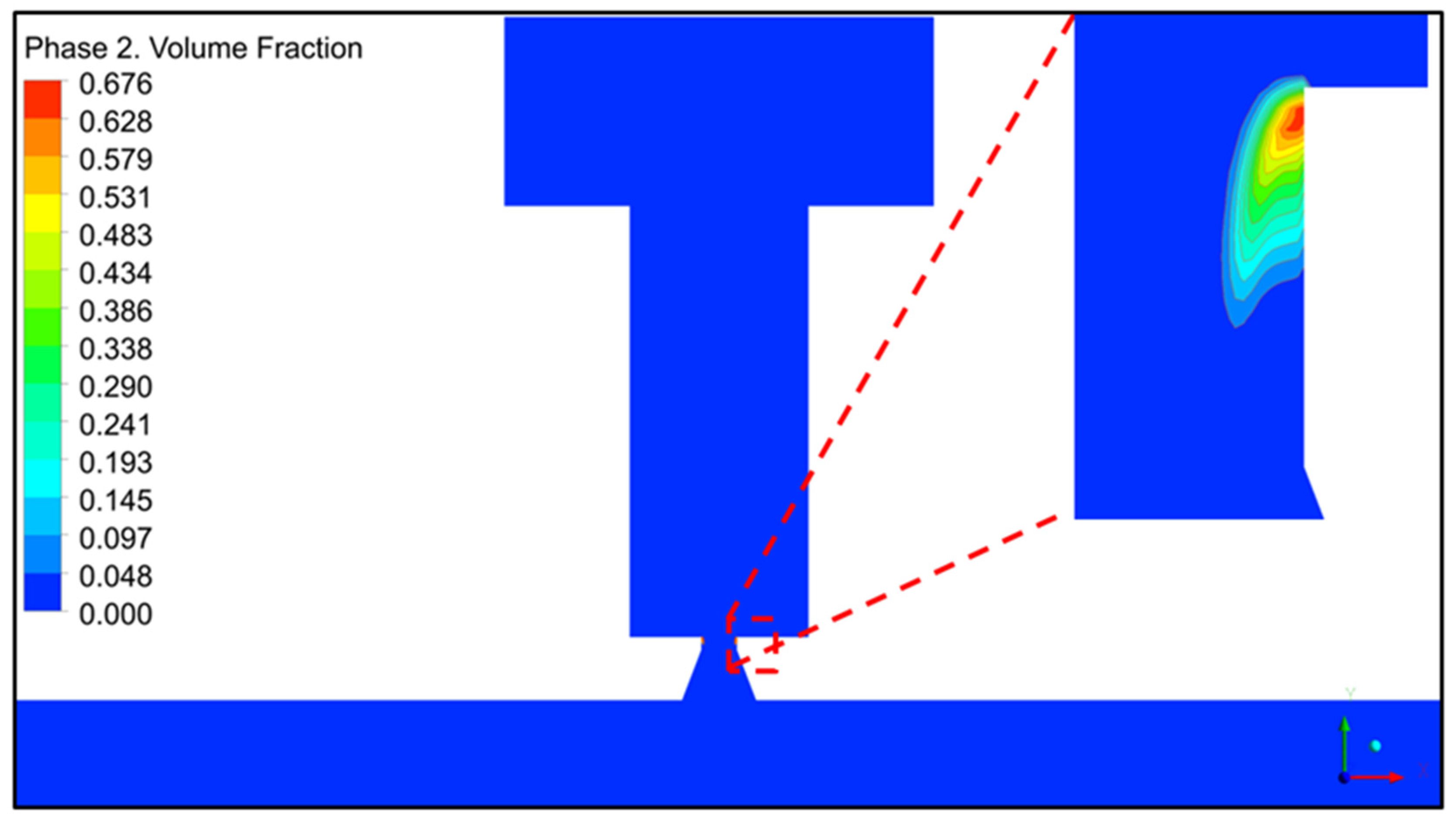
- (3)
- The results show that the vapor phase at the throat of the nozzle has the highest of the volume fraction, where the strongest cavitation in our research occurs. This shows that when the velocity vortexes appear and the pressure is lower than vapor pressure, the cavitation occurs.
Author Contributions
Funding
Acknowledgments
Conflicts of Interest
References
- Chahine, G.L.; Johnson, V.E.; Lindenmuth, W.T.; Frederick, G.S. The use of self-resonating cavitating water jets for underwater sound generation. J. Acoust. Soc. Am. 1985, 77, 113–126. [Google Scholar] [CrossRef]
- Lichtarowicz, A. Use of a Simple Cavitating Nozzle for Cavitation Erosion Testing and Cutting. Nat. Phys. Sci. 1972, 239, 63–64. [Google Scholar] [CrossRef]
- Chahine, G.L.; Kalumuck, K.M. Fluid Jet Cavitation Method and System for Efficient Decontamination of Liquids. U.S. Patent 09/285,864, 2 April 1999. [Google Scholar]
- Bai, F.; Wang, L.; Saalbach, K.-A.; Twiefel, J. A Novel Ultrasonic Cavitation Peening Approach Assisted by Water Jet. Appl. Sci. 2018, 8, 2218. [Google Scholar] [CrossRef] [Green Version]
- Peng, G.; Shimizu, S. Progress in numerical simulation of cavitating water jets. J. Hydrodyn. 2013, 25, 502–509. [Google Scholar] [CrossRef]
- Kang, C.; Liu, H.; Zhang, T.; Li, Q. Investigation of submerged waterjet cavitation through surface property and flow information in ambient water. Appl. Surf. Sci. 2017, 425, 915–922. [Google Scholar] [CrossRef]
- Li, D.; Chen, Y.; Kang, Y.; Wang, Z.; Wang, X.; Fan, Q.; Yuan, M. Experimental investigation of the preferred Strouhal number used in self-resonating pulsed waterjet. J. Mech. Sci. Technol. 2018, 32, 4223–4229. [Google Scholar] [CrossRef]
- Gopalan, S.; Katz, J.; Knio, O. The flow structure in the near field of jets and its effect on cavitation inception. J. Fluid Mech. 1999, 398, 1–43. [Google Scholar] [CrossRef] [Green Version]
- Peng, K.; Tian, S.; Li, G.; Alehossein, H. Mapping cavitation impact field in a submerged cavitating jet. Wear 2018, 396–397, 22–33. [Google Scholar] [CrossRef]
- Peng, C.; Tian, S.; Li, G. Joint experiments of cavitation jet: High-speed visualization and erosion test. Ocean Eng. 2018, 149, 1–13. [Google Scholar] [CrossRef]
- Belyakov, G.V.; Filippov, A.N. Cavitating vortex generation by a submerged jet. J. Exp. Theor. Phys. 2006, 102, 862–868. [Google Scholar] [CrossRef]
- Alehossein, H.; Qin, Z. Numerical analysis of Rayleigh–Plesset equation for cavitating water jets. Int. J. Numer. Methods Eng. 2007, 72, 780–807. [Google Scholar] [CrossRef]
- Pan, Y.; Tengfei, C.; Fei, M. Self-Excited Frequency Estimation Model of Organ-Pipe Waterjet under Confining Pressure. J. Mech. Eng. 2018, 54, 220–225. [Google Scholar] [CrossRef]
- Peters, A.; Sagar, H.; Lantermann, U.; el Moctar, O. Numerical modelling and prediction of cavitation erosion. Wear 2015, 338-339, 189–201. [Google Scholar] [CrossRef]
- Blake, J.R.; Leppinen, D.M.; Wang, Q. Cavitation and bubble dynamics: The Kelvin impulse and its applications. Interface Focus 2015, 5, 20150017. [Google Scholar] [CrossRef] [PubMed]
- Annoni, M.; Arleo, F.; Malmassari, C. CFD aided design and experimental validation of an innovative Air Assisted Pure Water Jet cutting system. J. Mater. Process. Technol. 2014, 214, 1647–1657. [Google Scholar] [CrossRef] [Green Version]
- Cai, T.; Liu, B.; Ma, F.; Pan, Y. Influence of nozzle lip geometry on the Strouhal number of self-excited waterjet. Exp. Therm. Fluid Sci. 2020, 112, 109978. [Google Scholar] [CrossRef]
- Asnaghi, A.; Svennberg, U.; Bensow, R.E. Analysis of tip vortex inception prediction methods. Ocean Eng. 2018, 167, 187–203. [Google Scholar] [CrossRef]
- Wu, Q.; Wang, C.; Huang, B.; Wang, G.; Cao, S. Measurement and prediction of cavitating flow-induced vibrations. J. Hydrodyn. 2018, 30, 1064–1071. [Google Scholar] [CrossRef]
- Karimi, A.; Al-Rashed, A.A.; Afrand, M.; Mahian, O.; Wongwises, S.; Shahsavar, A. The effects of tape insert material on the flow and heat transfer in a nanofluid-based double tube heat exchanger: Two-phase mixture model. Int. J. Mech. Sci. 2019, 156, 397–409. [Google Scholar] [CrossRef]
- Garoosi, F.; Rashidi, M.M. Conjugate-mixed convection heat transfer in a two-sided lid-driven cavity filled with nanofluid using Manninen’s two phase model. Int. J. Mech. Sci. 2017, 131–132, 1026–1048. [Google Scholar] [CrossRef]
- Wang, C.-C.; Huang, B.; Wang, G.-Y.; Duan, Z.-P.; Ji, B. Numerical simulation of transient turbulent cavitating flows with special emphasis on shock wave dynamics considering the water/vapor compressibility. J. Hydrodyn. 2018, 30, 573–591. [Google Scholar] [CrossRef]
- Díaz, A.; Alegre, J.M.; Cuesta, I.; Zhang, Z. Numerical study of hydrogen influence on void growth at low triaxialities considering transient effects. Int. J. Mech. Sci. 2019, 164, 105176. [Google Scholar] [CrossRef]
- Abe, K.; Kondoh, T.; Nagano, Y. A new turbulence model for predicting fluid flow and heat transfer in separating and reattaching flows-l. Flow field calculations. Int. J. Heat Mass. Tran. 1994, 37, 139–151. [Google Scholar] [CrossRef]
- Langhi, M.; Hosoda, T.; Subhasish Dey, M.A. Analytical Solution of k-ε Model for Nonuniform Flows. J. Hydraul. Eng. 2018, 144, 4018031–4018033. [Google Scholar] [CrossRef]
- Rohdin, P.; Moshfegh, B. Numerical predictions of indoor climate in large industrial premises. A comparison between different k–ε models supported by field measurements. Build. Environ. 2007, 42, 3872–3882. [Google Scholar] [CrossRef]
- Fu, C.; Uddin, M.; Robinson, A.C. Turbulence modeling effects on the CFD predictions of flow over a NASCAR Gen 6 racecar. J. Wind. Eng. Ind. Aerodyn. 2018, 176, 98–111. [Google Scholar] [CrossRef]
- Zhu, H.; You, J.; Zhao, H. Underwater spreading and surface drifting of oil spilled from a submarine pipeline under the combined action of wave and current. Appl. Ocean Res. 2017, 64, 217–235. [Google Scholar] [CrossRef]
- De Giorgi, M.G.; Ficarella, A.; Fontanarosa, D. Implementation and validation of an extended Schnerr-Sauer cavitation model for non-isothermal flows in OpenFOAM. Energy Procedia 2017, 126, 58–65. [Google Scholar] [CrossRef]
- Roohi, E.; Pendar, M.R.; Rahimi, A. Simulation of three-dimensional cavitation behind a disk using various turbulence and mass transfer models. Appl. Math. Model. 2016, 40, 542–564. [Google Scholar] [CrossRef]
- Wang, H.; Zhou, L.; Liu, D.; Karney, B.; Wang, P.; Xia, L.; Ma, J.; Xu, C. CFD Approach for Column Separation in Water Pipelines. J. Hydraul. Eng. 2016, 142, 04016036. [Google Scholar] [CrossRef] [Green Version]
- Chen, J.Q.; Chen, K.; Chen, X.M. Simulation analysis on inner flow field and optimization design of air knife. J. Vibroeng. 2017, 19, 6374–6389. [Google Scholar] [CrossRef]
- Tokgoz, N. Experimental and numerical investigation of flow structure in a cylindrical corrugated channel. Int. J. Mech. Sci. 2019, 157-158, 787–801. [Google Scholar] [CrossRef]
- Johnson, V.E.; Lindenmuth, W.T.; Chahine, G.L.; Conn, A.F.; Frederick, G.S. Research and Development of Improved Cavitating Jets for Deep-Hole Drilling; Hydronautics, Inc.: Laurel, MD, USA, 1984. [Google Scholar]
- Del Grosso, V.A. Speed of Sound in Pure Water. J. Acoust. Soc. Am. 1972, 52, 1442–1446. [Google Scholar] [CrossRef]
- Cui, L.; Ma, F.; Gu, Q.; Cai, T. Time–Frequency Analysis of Pressure Pulsation Signal in the Chamber of Self-Resonating Jet Nozzle. Int. J. Pattern Recognit. Artif. Intell. 2018, 32, 1858001–1858006. [Google Scholar] [CrossRef]
- Liu, W.; Kang, Y.; Zhang, M.; Wang, X.; Li, D.; Xie, L. Experimental and theoretical analysis on chamber pressure of a self-resonating cavitation waterjet. Ocean Eng. 2018, 151, 33–45. [Google Scholar] [CrossRef]
- Qin, Y.; Mao, Y.; Tang, B. Multicomponent decomposition by wavelet modulus maxima and synchronous detection. Mech. Syst. Signal Process. 2017, 91, 57–80. [Google Scholar] [CrossRef]
- Coccaro, N.; Ferrari, G.; Donsi, F. Understanding the break-up phenomena in an orifice-valve high pressure homogenizer using spherical bacterial cells (Lactococcus lactis) as a model disruption indicator. J. Food Eng. 2018, 236, 60–71. [Google Scholar] [CrossRef]
- Kang, C.; Liu, H.; Soyama, H. Estimation of aggressive intensity of a cavitating jet with multiple experimental methods. Wear 2018, 394-395, 176–186. [Google Scholar] [CrossRef]
- Sou, A.; Hosokawa, S.; Tomiyama, A. Effects of cavitation in a nozzle on liquid jet atomization. Int. J. Heat Mass Transf. 2007, 50, 3575–3582. [Google Scholar] [CrossRef] [Green Version]


| Phases | Fluid Density kg/m3 | Viscosity Kg/m-s | Surface Tension N/m |
|---|---|---|---|
| Water | 998.2 | 0.001003 | 0.072 |
| Vapor | 0.5542 | 1.34 × 10⁻⁵ |
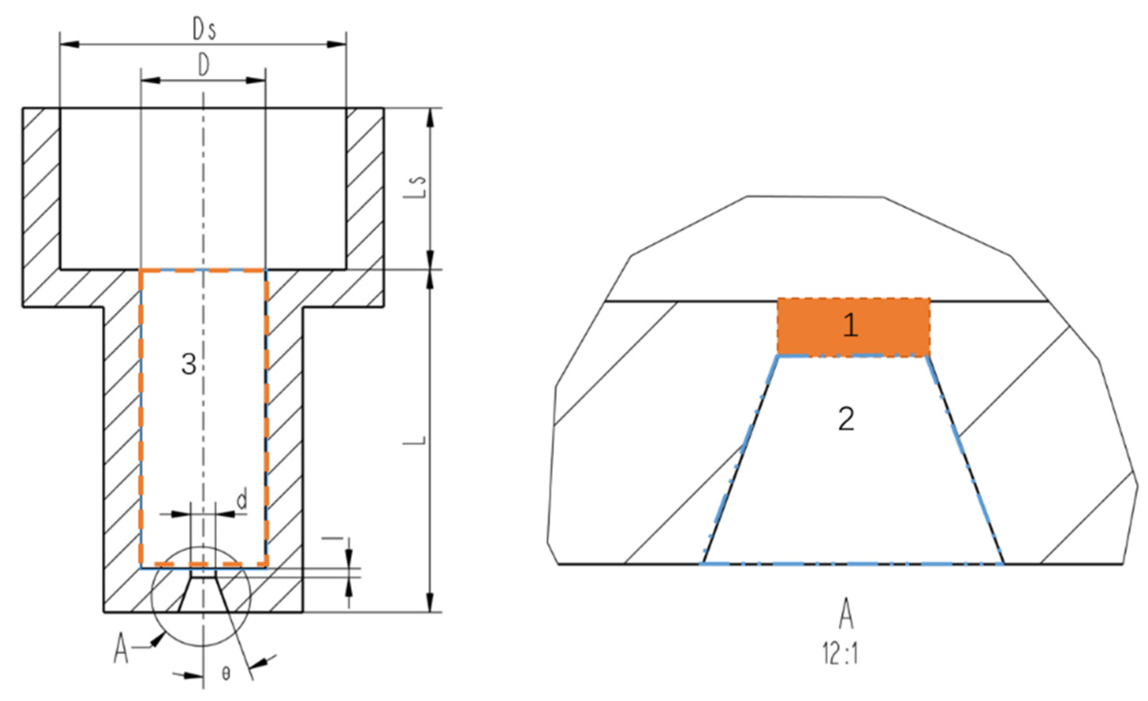
| Ds/mm | D/mm | L/mm | d1/mm | l1/mm | Θ (°) |
|---|---|---|---|---|---|
| 23 | 10 | 24 | 2 | 0.7 | 21 |
| i | 1 | 2 | 3 | 4 |
|---|---|---|---|---|
| fe(i) | 2894 | 5992 | 11,960 | 17,880 |
| fs(i) | 2934 | 4961 | 9942 | 14,900 |
| Ea(i) | 1.3% | 17.2% | 16.88% | 16.7% |
Publisher’s Note: MDPI stays neutral with regard to jurisdictional claims in published maps and institutional affiliations. |
© 2021 by the authors. Licensee MDPI, Basel, Switzerland. This article is an open access article distributed under the terms and conditions of the Creative Commons Attribution (CC BY) license (https://creativecommons.org/licenses/by/4.0/).
Share and Cite
Cui, L.; Ma, F.; Cai, T. Investigation of Pressure Oscillation and Cavitation Characteristics for Submerged Self-Resonating Waterjet. Appl. Sci. 2021, 11, 6972. https://doi.org/10.3390/app11156972
Cui L, Ma F, Cai T. Investigation of Pressure Oscillation and Cavitation Characteristics for Submerged Self-Resonating Waterjet. Applied Sciences. 2021; 11(15):6972. https://doi.org/10.3390/app11156972
Chicago/Turabian StyleCui, Lihua, Fei Ma, and Tengfei Cai. 2021. "Investigation of Pressure Oscillation and Cavitation Characteristics for Submerged Self-Resonating Waterjet" Applied Sciences 11, no. 15: 6972. https://doi.org/10.3390/app11156972