1. Introduction
As one of the core pieces of equipment, the transformer directly affects the safe, efficient and economic operation of the power system, so it is especially important to ensure the safe and stable operation of the transformer. Partial discharge (PD) is the main cause of transformer insulation damage, and the effect of different types of partial discharge on the transformer insulation system is different, so it is of great practical significance to effectively identify the discharge pattern and take corresponding measures [
1,
2].
The traditional PD pattern recognition method mainly includes three parts, which include obtaining the PD data, extracting the PD features and training the pattern recognition classifier [
3]. Scholars have done a lot of research on the feature extraction and pattern recognition classifier. The common characteristic parameters include statistical parameters, waveform parameters, fractal characteristic parameters, wavelet parameters, moment characteristic parameters and so on [
4,
5,
6,
7,
8,
9]. For pattern recognition methods, back-propagation neural network (BPNN) and support vector machine (SVM) are widely used [
10,
11,
12]. However, these machine learning algorithms, which rely on the artificial construction of PD features, are highly subjective and have large recognition errors [
13].
With the development of artificial intelligence and computer vision technology, the application of deep neural network to PD pattern recognition can be used to overcome the shortcomings of traditional methods. Although the convolutional neural network (CNN) has the advantage of requiring no artificial computation of signal features, it has not been widely used in the PD pattern recognition. At present, the basic research of CNN includes analyzing the performance differences of convolutional network under different layers, activation functions and pooling modes.
The CNN model has a better recognition effect, which improves the accuracy compared with SVM and BPNN [
14]. Some literature uses the time domain waveform image of PD as data samples to conduct supervised training on the constructed one-dimensional CNN model [
15]. In addition, PRPS spectra obtained from the field experiments and simulation are used as input data, and classical CNN model LeNet-5 is used as classifier [
16]. However, these models have fewer layers and cannot fully extract the PD features. The depth model has good recognition accuracy, but it has a large number of parameters and high complexity in terms of model size, which leads to huge network capacity, slow operation speed and high computational resource consumption. Therefore, it is not suitable to embed the deep learning models into devices and it is difficult to deploy them on miniaturized hardware platforms.
In order to solve the above problems, a transformer PD pattern recognition method based on MobileNets convolution neural network model is proposed. The model introduces the lightweight attention mechanism Squeeze—and—Excitation (SE) module and h-swish activation function with stronger nonlinear performance based on the use of depth separable convolution module and inverse residual structure. Then, the MCNN network is trained and tested by different types of PD data obtained from laboratory experiments. Analysis results show that the MCNN can significantly reduce the number of parameters and the computational complexity of the model. In addition, MCNN can further improve the recognition accuracy compared with the existing convolutional neural network, which is often used for PD type classification. Finally, the feature maps of the convolution output of the last layer in the MCNN are visually calculated to explain the classification process and verify the function of the model.
The remainder of this paper is organized as follows. Data acquisition of PD in transformer is illustrated in
Section 2.1; then, the CNN and NCNN (noisy convolution neural network) principle methodology are introduced in
Section 2.2. Mobilenets Convolution Neural Network is illustrated in
Section 2.3, and Lightweight MCNN Block is shown in
Section 2.4. Training and Testing of MCNN are given in
Section 2.5.
Section 3 highlights the MCNN with a discussion about the experimental results and the comparison with a few previous pattern recognition methods. Finally, conclusions of the paper are given in
Section 4.
2. PD Pattern Recognition Based on MCNN
2.1. PD Data Acquisition of Transformer
According to the common types of insulation defects in transformer operation, four typical PD models are made. These PD models are used to simulate the transformer tip discharge, surface discharge, air gap discharge and suspended discharge. In the experiment, a PD detection system based on ultra-high frequency (UHF) sensors is used. The sampling rate of the system is 4 GHz, and the bandwidth is 1 GHz.
During the experiment, the voltage is stepped up and (UHF) sensors are used to collect PD data from the four PD models. The collected PD data is used to build a sample database of PRPD maps for subsequent feature extraction and pattern recognition. The specific test steps are listed as follows:
- (1)
A PD insulation defect model is selected and connected to the partial discharge test circuit.
- (2)
The background noise of the laboratory is determined. Before the voltage is applied, the signal detected by the signal acquisition system is the background noise of the PD test environment.
- (3)
The inception voltage of the PD is determined. The voltage of the regulating transformer is increased uniformly and slowly in steps. When the PD signal is detected by the monitoring instrument, the corresponding voltage is recorded as the initial voltage U1.
- (4)
The PD data is generated and collected at different voltage supplies. The voltage is continuously increased, and when it is greater than 1.5 times U1, a stable and distinct PD signal series is recorded in the monitoring system. The voltage is then still increased to approximately twice U1. The PD data generated during this process is collected by the UHF sensors. The sensors can record the partial discharge signals of different intensities generated by the partial discharge model at different voltage levels.
- (5)
Different types of insulation defect models are replaced. After completing the PD test of the current PD insulation defect model, the voltage is slowly lowered and the power is turned off. Different types of insulation defect models are replaced. After completing the PD test for the current PD insulation defect model, the voltage is slowly reduced and the power is turned off. The discharge bar is used to discharge the test circuit, and the insulation defect model is replaced with another one. Then, the experiment steps (2) to (5) are then repeated until all four types of PD data are collected.
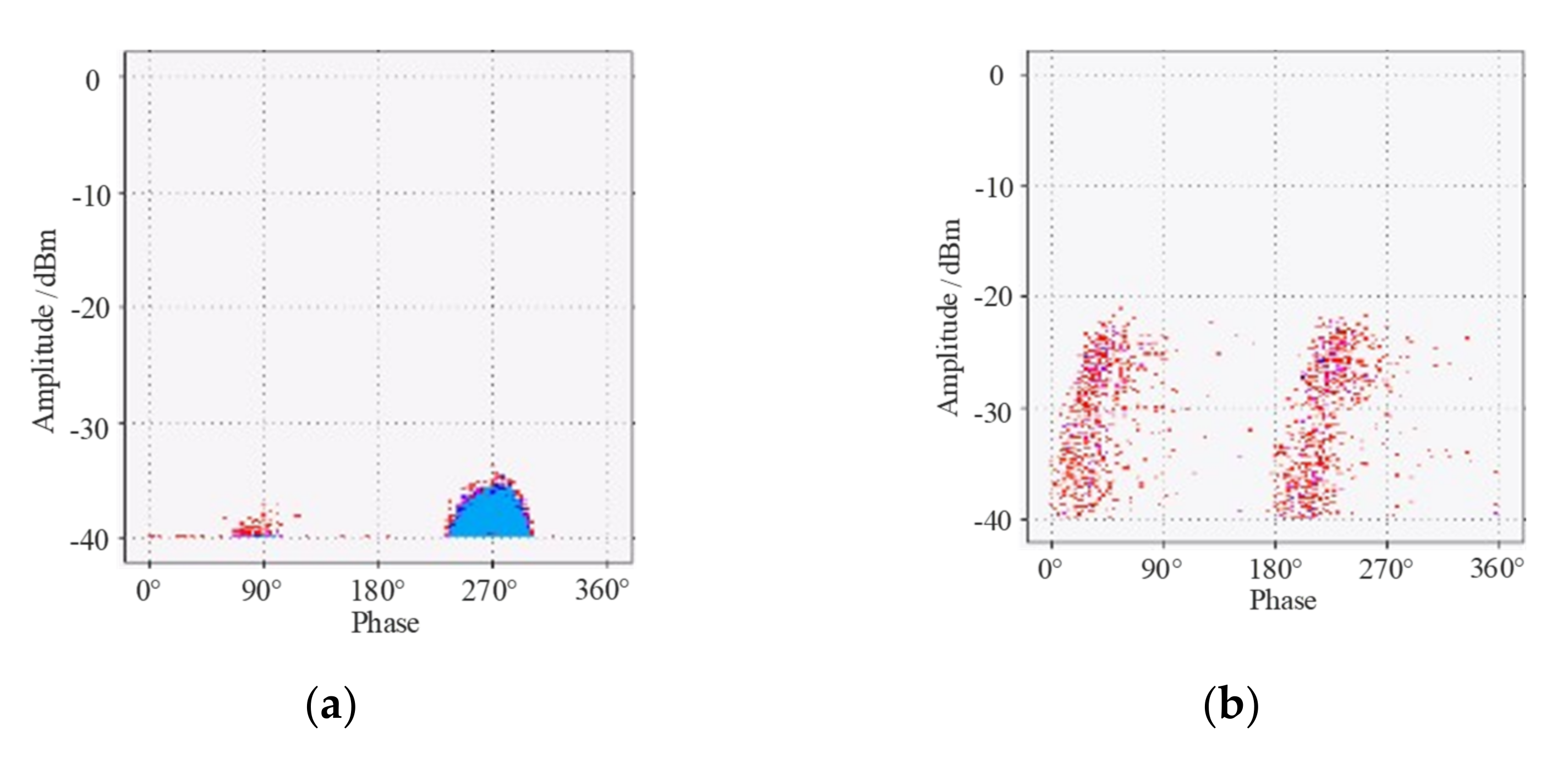
The PRPD spectra obtained from the PD test are shown in
Figure 1, in which each spectrum contains 50 power frequency cycles of discharge data. In the PRPD spectra, by observing the vertical and horizontal coordinates of a pulse point, we can directly obtain information about the phase and amplitude of the pulse.
In the experimental process of the tip discharge model, with the increase of applied voltage, a cluster of PD signals appear at the positions with the phase of 270°. This is because in 50 Hz AC, the AC voltage peaks at 270° in phase. The electrons are most active and more easily repelled at the moment when the voltage is at a negative peak, which coincides with the easy excitation of a negative polarity tip. With the further increase of voltage, the second cluster discharge signal appeared at the 90° phase position. This is because the voltage reaches a positive peak at 90° phase. When the voltage applied on the conductor is positive polarity, more energy is required for electron excitation, so the overall discharge amplitude at this time is lower than the first cluster signal at position 270°. Furthermore, the distribution phase width is narrower than that at position 270°.
Suspended discharge is produced by suspended potential. Taking loose bolts as an example: when bolts and conductors are not in contact, the voltage at both ends of the middle gap is the same. In this case, high energy will be released when PD occurs, resulting in a high discharge amplitude and a consistent discharge height. This is an obvious distribution characteristic of suspended discharge. In addition, in the PRPD spectra, both air gap discharge and surface discharge are evenly distributed signals with different amplitudes and wide phase distributions. It can be seen that the distribution of discharge points in the PRPD spectra of different types of partial discharges varies greatly, and this distribution difference can be translated into pixel space distribution features that can be processed and extracted by CNN for pattern recognition.
2.2. Convolution Neural Network
Convolution neural network (CNN) is a deep learning framework, which is proposed by the mechanism of the biological receptive field and developed rapidly in computer vision. The CNN reduces the parameters of model training and extracts the relevant semantic features of the input image effectively using sparse connectivity and weights sharing. A typical CNN structure consists of one input layer, one or more alternately connected convolution and pooling layers, a full connection layer, and an output layer. The input image is first processed continuously through the convolutional layer and pooling layer; then the input image is classified in the full connection layer; and, finally, the recognition result is output.
The convolution layer contains multiple convolution kernels, each of which is a filter to extract the features of the input data. Each neuron in the convolution layer is connected with the local receptive field of the upper layer, and the convolution operation is carried out to determine the relationship of each feature. The formula is shown in (1):
where
f is the activation function and
is the convolution operation.
the step is the output feature of the previous convolution layer.
is the set of input feature maps,
ω is the convolution kernel, b is the offset value of each map, and
l is the number of network layers.
The function of the pooling layer is used for down-sampling operation, which can select the output of the feature from the convolution layer, thus reducing the feature dimension. The nonlinear activation function is added between the convolutional layer and the pooling layer to improve the expression ability of the model. Common activation functions include Sigmoid, Tanh, and ReLU. In the fully connected layer, the final feature maps are reorganized into lower-dimensional vectors for the training and classification.
2.3. Mobilenets Convolution Neural Network
With the continuous increase of the number of layers of convolution neural network, the number of parameters and the amount of calculation also increase. This leads to a complex model structure and slow computing speed, which is not conducive to the application and development of CNNs in the field of pattern recognition with real-time online requirements. To solve these problems, Google proposed the MobileNets convolution neural network (MCNN) in 2017 [
17]. A Depthwise Separable Convolution structure is used in the unit block of the model, which greatly reduces the number of parameters and computation of the model and achieves more efficient performance through the reverse residual structure with a linear bottleneck. On this basis, we add the Squeeze-and-Excitation structure to the model used in the paper and adjust the activation function to further improve the learning ability and timeliness of the model [
18].
In the MobileNets model, the depth separable convolution is used instead of traditional standard convolution. Depth separable convolution mainly includes two parts: depth convolution and 1 × 1 point convolution [
19]. This decomposition is linear, which can reduce the computation and model parameters, as shown in
Figure 2.
Figure 2a is the traditional standard convolution, the number of convolution kernels is N, and the number of input channels is M. The traditional standard convolution can be decomposed into the sum of the depth convolution shown in (b) and the point-by-point convolution shown in (c). The MobileNets can reduce the number of parameters and improve the computational efficiency by using the depth separable convolution structure.
Theoretically, the recognition effect of the model with more layers of the network will be better. But practical experience shows that the difficulty of network training and optimization increases with the increase of layers, which leads to network degradation, and the effect will be worse than that of the relatively shallow network. In the traditional residual structure shown in
Figure 3, the above problem is solved by introducing a shortcut connection structure. The dimension of the feature channel is first reduced to the lower dimension and extracted features, then extended to the high dimension. To improve the classification performance of the network and alleviate the problem of gradient vanishing in multi-layer backpropagation, the reverse residual structure with linear bottleneck is introduced into the MobileNets, as shown in
Figure 4. The feature channel dimension in the reverse residual structure is first extended to the higher dimension to extract features and then reduced to the lower dimension. This structure can increase the nonlinear expression capacity of each feature channel by deep convolution in the high-dimensional feature space and maintain the compact feature expression in the input and output information, which makes the structure of the model more efficient.
The feature transfer in the traditional convolution network is to transfer the weight of the feature graph to the next layer, and the Squeeze-and-Excitation (SE) module can adaptively correct the importance of features between channels according to the global loss function of the network, to increase the weight of effective features. This structure can strengthen the learning ability of the network and improve the accuracy of the model by strengthening the important features.
2.4. Lightweight MCNN Block
The lightweight and efficient convolution module adopted in the MCNN is shown in
Figure 5. Firstly, the number of input feature channels is extended to a large number of intermediate layers by 1 × 1 point convolution, then features are extracted and optimized by 3 × 3 depth convolution. Finally, 1 × 1 point convolution is used to compress the features to the size given by the output channel. The specific implementation of each module of constructing this convolution network corresponding to
Figure 6 is shown in
Table 1. The number of input channels of the convolution module is N, and the number of output channels is M. For the input feature of a certain size W × H, the expansion factor is
t, the convolution kernel size is 3,
s denotes stride, and NL denotes the nonlinear function.
Table 2 shows the overall structural parameters of the compact and computationally efficient lightweight MCNN. The rows in
Table 2 describe the specific structural configuration of each convolution layer in the model [
19]. The size of the input data of the first layer is 224 × 224 × 3, in which 3 represents the 3-channel image in RGB format. The standard convolution operation is carried out on this input data, in which the number of channels of the kernel is set to 16, which can minimize the operation time on the premise of ensuring accuracy. The 2nd to 12th convolution layers in
Table 2 all adopt the reverse residual module with a linear bottleneck. The 13th layer is point-by-point convolution. The 14th layer is the pooling layer, which converts the output feature from the convolution layer pooling to 1 × 1 × 576. Then, the fully connected layer is used to reconstruct the final feature image into a lower-dimensional vector. Finally,
k types of identification information are output in the 16th layer.
The “conv2d” in the
Table 2 denotes the two-dimensional convolution operation; the “Bneck” is the bottleneck structure, the “NBN” indicates that the batch is not normalized, and the module with “SE” lightweight attention structure is marked in the “SE” column. The type of non-linear used in each convolution layer is introduced in “NL”, in which “HS” means to use h-swish, “RE” means to use standard ReLU6.
In some convolution layers of MCNN, h-swish is used to replace swish. This is because although swish can effectively improve the accuracy of the network, it will lead to a large amount of calculation and is takes too much time to contain the sigmoid function due to its characteristics of no upper bound and lower bound, and non-monotonicity. The h-swish can not only better approximate the original swish to reduce the amount of computation but can also improve the computational efficiency in the quantization mode, which makes the model more suitable for the embedded, low-power environment. The mathematical definitions of the swish and the h-swish are as follows.
x is the input signal.
2.5. Training and Testing of MCNN
In this paper, MCNN is used to identify the type of PD in the transformer. To further improve the performance of the model and avoid over-fitting, we first expand the PD data obtained, to effectively increase the number and diversity of training samples. In the output layer of the model, the SoftMax is used as the classifier, and the one-hot encoding is used to encode the categories of four types of PD. The specific steps of PD pattern recognition of transformer based on MCNN are as follows:
- (1)
Data acquisition. According to the data collected by the discharge experiment, the PRPD spectrum is generated, and the collected PD images are randomly divided into the training set and test set, accounting for 80% and 20% of the total samples respectively.
- (2)
Data preprocessing. Firstly, the PRPD spectrum of PD is randomly allocated to obtain a 224 × 224 × 3 three-channel RGB image, and then the image is flipped randomly and converted into a floating-point tensor with a value between 0~1.
- (3)
Data enhancement. The sample of the original data is expanded, including random rotation, segmentation, scaling, and other operations. To improve the generalization ability of the model, 20% of the training data is randomly selected by using data enhancement for image generation.
- (4)
Data standardization. To establish the comparability of the data, the standardized method is used to normalize the input data.
- (5)
Model training. The loss function used in the training process is the Cross-Entropy Loss, and the optimization algorithm adopted is the Stochastic Gradient Descent. Dropout and Batch Normalization are used to improve the training performance.
- (6)
Model testing. The trained model is tested on the test set. The purpose of the model testing phase is to verify the generalization ability of the model, and the recognition accuracy of the model to PD data can be obtained.
The overall flow chart of PD recognition based on the MobileNets convolution neural network designed above is shown in
Figure 6.
4. Conclusions
In this paper, a method to identify the transformer PD patterns based on MobileNets convolution neural network (MCNN) is designed. Based on adopting a deep separable convolution module and inverse residual structure, the basic module of MCNN introduces lightweight attention mechanism SE module and h-swish function with stronger nonlinear ability, which can effectively avoid the problems such as the need for human intervention and low recognition rate existing in the traditional shallow learning algorithm. In addition, the model solves the defects of the current depth model applied in PD pattern recognition, such as high complexity, a large number of parameters, large memory, and slow running speed.
The MCNN is trained and tested through different types of PRPD spectra obtained by experiments, and the classification performance of the model is compared with many existing deep convolution neural network models and compression network models. A variety of visualization methods are used to further understand the internal solution process of the MCNN model and explain the feasibility of the model in PD recognition. The results show that the MCNN can significantly reduce the number of parameters and the computational complexity of the model, and at the same time, further improve the accuracy of PD type recognition. Therefore, PD pattern recognition based on the model can be used in small mobile devices or integrated systems, and alleviate the pressure of space resources shortage on offshore platforms.


