Article

Exploiting Spatial Information to Enhance DTI Segmentations via Spatial Fuzzy c-Means with Covariance Matrix Data and Non-Euclidean Metrics

1
Department of Mathematical Sciences, Loughborough University, Loughborough LE11 3TU, UK
2
School of Computing, Engineering and Mathematics, University Brighton, Brighton BN2 4GJ, UK
*
Author to whom correspondence should be addressed.
These authors contributed equally to this work.
Appl. Sci. 2021, 11(15), 7003; https://doi.org/10.3390/app11157003
Submission received: 30 May 2021 / Revised: 20 July 2021 / Accepted: 26 July 2021 / Published: 29 July 2021
(This article belongs to the Topic Medical Image Analysis)

Abstract

:
A diffusion tensor models the covariance of the Brownian motion of water at a voxel and is required to be symmetric and positive semi-definite. Therefore, image processing approaches, designed for linear entities, are not effective for diffusion tensor data manipulation, and the existence of artefacts in diffusion tensor imaging acquisition makes diffusion tensor data segmentation even more challenging. In this study, we develop a spatial fuzzy c-means clustering method for diffusion tensor data that effectively segments diffusion tensor images by accounting for the noise, partial voluming, magnetic field inhomogeneity, and other imaging artefacts. To retain the symmetry and positive semi-definiteness of diffusion tensors, the log and root Euclidean metrics are used to estimate the mean diffusion tensor for each cluster. The method exploits spatial contextual information and provides uncertainty information in segmentation decisions by calculating the membership values for assigning a diffusion tensor at one voxel to different clusters. A regularisation model that allows the user to integrate their prior knowledge into the segmentation scheme or to highlight and segment local structures is also proposed. Experiments on simulated images and real brain datasets from healthy and Spinocerebellar ataxia 2 subjects showed that the new method was more effective than conventional segmentation methods.

1. Introduction

Brain image classification and region segmentation methods are crucial components in medical applications. The Corpus Callosum (CC) is a great fibre bundle in the white matter of the brain that connects the two hemispheres of the brain. A change in the size and shape of the CC can be indicator of a brain abnormality [1,2,3], and hence an accurate segmentation of the CC is important in the diagnosis of disease and for surgical planning. Automating the production of accurate segmentations is a crucial step in saving a significant amount of clinician time in practice by removing the need for manual segmentation.
Diffusion Tensor Imaging (DTI) is an advanced magnetic resonance imaging technique that measures the Brownian displacements of water molecules in each voxel in the brain [4], providing unique information about biological tissues in the brain. A diffusion tensor (DT) is a 3 × 3 real positive semi-definite covariance matrix [5] that describes the mobility of molecules in each direction. Therefore, the dimensions of a DTI dataset are five for 2D images and six for 3D images (i.e., including the spatial location dimensions). Analysing the DTI data itself, as 4D or 5D, retains all the information from the data with no loss of diffusivity information.
The space of positive semi-definite covariance matrices arises in many applications, such as in image and longitudinal data analysis, and thus methods developed for covariance matrices are more widely applicable than medical imaging. To measure distance in the space of positive semi-definite covariance matrices, various non-Euclidean metrics [6,7] have been proposed as alternatives to the Euclidean metric to avoid violations of the positive semi-definiteness criterion in the course of extrapolation, for example, and since Euclidean averaging is prone to swelling (i.e., inflation of the determinant [7]).
Computing a mean using certain non-Euclidean metrics (e.g., Procrustes and Riemannian) require numerical solutions to be solved, whilst other non-Euclidean metrics (e.g., log Euclidean, root Euclidean, and Cholesky) do not; not requiring numerical methods tends to be computational faster, which is an important criterion for practical medical applications due to the large data sets. Diffusion Tensor indices, such as Fractional Anisotropy (FA) and Mean Diffusivity (MD), are sensitive to brain abnormalities; the FA values of the CC have been reported to be decreased and MD values to be increased in abnormal brains as compared to healthy brains [8,9,10].
Spinocerebellar ataxia 2 (SCA2) is a particular hereditary neurodegenerative disorder [11] caused by progressive dysfunction of the cerebellum and the brain stem, and it is characterized by progressive problems with movement. DTI has been found to be useful for assessing microstructural changes in the brain white matter, which are associated with SCA2 [12,13,14]. The authors in [15] used FreeSurfer software for the segmentation of the cerebrum and the brainstem-cerebellum, and performed a histogram analysis of the DTI indices of FA, MD, radial diffusivity (RD), axial diffusivity (AX), and mode of anisotropy (MO). The FA and MO values were decreased whilst the MD, RD, and AX values were increased in SCA2 subjects compared to healthy brains. Thus, all of these indices can be used for disease diagnosis from suitably segmented images.
Traditional image processing methods use scalar and vector-valued data for data analysis. In particular, spatial fuzzy c-means (sFCM) improves the segmentation of images (in comparison with K-means) by using the neighbouring information to minimize the effect of noise [16]. The standard sFCM algorithm uses Euclidean distance and the Euclidean mean to cluster sets of vectors and needs adaptation to be applicable for use with matrix-based data. To cluster sets of covariance matrices, such as diffusion tensors, a K-means algorithm was adapted for use by the authors in [17]; using a single manually segmented image as ground truth, the log Euclidean and Riemannian metrics were found to provide the most accurate segmentations of the CC (using accuracy and specificity as performance measures).
As a significant step forward, a spatial fuzzy c-means (sFCM) clustering method for covariance data (so that we do not loose information from the diffusion tensors), which effectively segment DT images by accounting for the noise, partial voluming, magnetic field inhomogeneity, and other imaging artefacts, was developed in the paper. To retain the non-Euclidean nature of DTs, the efficiently computable log and root Euclidean metrics are used to estimate the mean DT for each cluster.
The results are compared with a baseline of K-means to the suitably adapted sFCM algorithm for clustering sets of covariance matrices. Simulation studies are designed to test the performance of the algorithms and the metrics in the face of increasing noise levels, which is an important aspect of automated segmentations in this domain; since simulations ensure that the CC as ground truth is determined, performance measures (the accuracy, specificity, sensitivity, precision, Gmean, and F-measure) can be calculated, and sFCM with the efficiently computable metrics compared to the baseline K-means algorithm with the same metrics.
The findings indicate that sFCM is better than K-means with the same metric for almost all noise levels and performance measures; almost always sFCM with the root Euclidean metric is the preferred option. To further explore use in practice, the segmentation method is also applied to the CC for real brain data from healthy and Spinocerebellar ataxia 2 (SCA2) subjects. This is unannotated real data (i.e., the CC has not already been annotated/indicated by a clinician), and thus one can make use of the fact that the CC is known to be a well-connected single white tract in order to determine the efficacy of the segmentation method in practice; since there should not be extra small regions or outliers appearing in the same cluster, disconnected voxels in the segmentation results can be considered as noise.
The findings indicate that the number of voxels that are incorrectly labelled as being within the CC is significantly smaller using sFCM versus K-means in this real data application. The paper also presents additional results that point to future utility and developments, such as: the determinant can be used to distinguish healthy and SCA2 subjects, the determinant can be used as a DTI index, which distinguishes between healthy and SCA2 subjects and is sensitive to ageing effects, and that the method can be used for more general classification tasks.
In terms of presentation, the base algorithms FCM and sFCM, adapted for covariance matrices, are described in Section 2. Basic matrix operators of a positive definite covariance matrix are described in Appendix A. The main content of the set-up and results obtained using the simulation studies and real brain data experiments are presented in Section 3. A block diagram indicating an overview of the processing steps and software used is presented in Appendix B. Our conclusions are presented in Section 4.

2. Materials and Methods

In this section, the non-Euclidean metrics used in the paper are described, and the adaptation of K-means for use with covariance matrices from [17] is recalled. Clustering, grouping a set of objects, can be hard or soft (fuzzy). In hard clustering, each object belongs to only one cluster whereas objects can belong to more than one cluster in soft clustering. The most common used methods for hard and soft clustering are K-means and FCM, respectively.
Recall that a covariance matrix is a square, symmetric, positive semi-definite matrix. Let D ( A j , A ¯ i ) represent the distance between the covariance matrices A j and A ¯ i where A ¯ i is the weighted mean of the covariance matrices in the cluster i. The distance D ( A j , A ¯ i ) and weighted mean A ¯ of the set A using Euclidean, log Euclidean, and root Euclidean metrics [6] are presented in Table 1 and Table 2, with details on how to compute the power, log, and exp relegated to Appendix A.
These metrics are the ones considered in this paper since the computation of their mean is faster (since there is no need to use numerical solutions) in comparison to non-Euclidean metrics (Procrustes and Riemannian) that do need numerical solutions. The computation of numerical solutions can be very time consuming, especially when processing large datasets, which violates a key requirement for most medical applications (i.e., efficiency).
Furthermore, the Log Euclidean metric provides similar results to Riemannian [18] and the root Euclidean metric provides similar results to Procrustes [7]. The Cholesky metric is another standard non-Euclidean metric; however, its use is omitted because, whilst the computation of the Cholesky mean does not need numerical solutions, the Cholesky metric is not as reliable as the others due to not being invariant under orthogonal transformations [7].

2.1. Hard Clustering for Covariance Matrices

One of the most commonly used hard clustering algorithms is the K-means algorithm, which aims to minimize the within-cluster sum of squares (WCSS). For a set of covariance matrices A = A 1 , , A n , the WCSS is given by [19]:
WCSS = j = 1 n i = 1 c D ( A j , A ¯ i ) 2 .
The K-means algorithm for clustering covariance matrices is shown in Algorithm 1.
Algorithm 1: K-means Algorithm
Applsci 11 07003 i001

2.2. Soft Clustering for Covariance Matrices

In soft clustering, data points can belong to more than one cluster with a specified membership for each cluster. One of the most widely used algorithms for soft clustering is Fuzzy c-means (FCM). The FCM algorithm aims to minimize the sum of weighted square distances within each cluster (WCSS). For a set of vectors x = x 1 , , x n , this is defined as follows [19]. Let m R with m 1 be the fuzzification parameter. Then,
WCSS = j = 1 n i = 1 c w i j m x j x ¯ i 2 , where x = t r a c e ( x x ) ,
w i j = 1 k = 1 c x j x ¯ i x j x ¯ k 2 m 1 , and x ¯ i = j = 1 n w i j m x j j = 1 n w i j m .
The membership (or weight) w i j represents the probability of x j belonging to cluster i, i 1 , , c and it satisfies 0 w i j 1 and i = 1 c w i j = 1 . The K-means algorithm can be recovered from FCM by appropriately setting the membership w i j values to 0 s or 1 s.
In this paper, the natural generalisation is proposed for the use of covariance matrices, by replacing the vectors x = x 1 , , x n with covariance matrices A = A 1 , , A n and using D ( A j , A ¯ i ) 2 in place of x j x ¯ i 2 as follows:
WCSS = j = 1 n i = 1 c w i j m D ( A j , A ¯ i ) 2 , where
w i j = 1 k = 1 c D ( A j , A ¯ i ) D ( A j , A ¯ k ) 2 m 1 .
The sFCM algorithm [16] uses the neighbouring information to improve clustering and reduce noise. The current paper’s generalised version for covariance matrices is provided directly. If A j is the covariance matrix for a voxel v, then let NB ( A j ) denote the set of covariance matrices of v’s neighbouring voxels. Define h i j as follows [16]:
h i j = k NB ( A j ) w i k .
Therefore, h i j represents the sum of the memberships of the neighbouring voxels NB ( A j ) . The size of the neighbourhood can vary. For 2D segmentation, a reasonable choice is to take NB ( A j ) as either a 3 × 3 or a 5 × 5 window around A j , whilst, for 3D segmentation, take a 3 × 3 × 3 or a 5 × 5 × 5 window. Next, the membership w i j in Equation (4) is replaced with the spatial membership z i j as follows:
WCSS = j = 1 n i = 1 c z i j m D ( A j , A ¯ i ) 2 , where
z i j = w i j p h i j q k = 1 c w k j p h k j q .
Here, the parameters p and q enable the fine control of the influence of the membership function w i j and the function h i j , respectively. For example, in noisy regions q can be increased to increase the influence of neighbouring voxels. When the clustering region is homogenous, z i j has similar value to w i j , whilst z i j is smaller than w i j if A j is considered ‘noise’ (i.e., it is not actually a member of the cluster i). FCM can be recovered from sFCM by choosing p = 1 and q = 0 . The sFCM adapted for covariance matrices is described in Algorithm 2.
The stopping condition z i j ( r ) z i j ( r 1 ) < ε in Step 2 of the sCFM algorithm captures that the change in spatial membership values has become suitably small. An alternative stopping criteria that can be used in Step 2 of the sFCM algorithm would be D ( A ¯ i ( r ) , A ¯ i ( r 1 ) ) < ε , capturing instead that the change in cluster centres has become suitably small, whilst taking account of the use of non-Euclidean metrics. The value of ε should be taken to be very small (e.g., it should be smaller than 0.1 × 10 8 , which is a possible value of diffusion in a given direction).
Additionally, the paper presents a regularisation model for sFCM. The WCSS for the regularisation model is defined as
RWCSS = j = 1 n i = 1 c z i j m D 1 ( A j , A ¯ i ) r 1 + λ i = 1 c D 2 ( A i , A ¯ i ) r 2 ,
Algorithm 2: sFCM Algorithm
Applsci 11 07003 i002
Here, λ > 0 is a regularisation parameter, r 1 , r 2 0 , and A i is a reference tensor representing the prescribed diffusion information for cluster i. Users of the technique have the option to either define their own reference tensor for cluster i with the expressed diffusion behaviour or choose a representative tensor from the cluster as the reference tensor. The proposed regularisation model allows the user to integrate their prior knowledge into the segmentation scheme or to highlight and segment local structures. Note that D 1 and D 2 need not be the same and can be non-Euclidean. When r 1 = 2 , λ = 0 , R W C S S simplifies, reducing to be equivalent to sFCM in [16].
In this work, after experimentation with the effects of varying the initial parameter values on segmentations of the CC, m = 2 , p = 2 , q = 1.5 and λ = 0 (for simplicity) with a 3 × 3 window for 2 D segmentation and a 3 × 3 × 3 window for 3 D segmentation were chosen; these values yielded are used consistently for both the simulation studies and the real data experiment in the following sections.
Finally, whilst Table 1 and Table 2 show only the Euclidean, log, and root Euclidean distances and means, any other suitable distance and mean (i.e., Cholesky, Riemannian, or Procrustes) can be used with the algorithm.

3. Results

In this section, the results obtained from experiments in the form of two simulation studies and one study using real brain data are described. The two simulation studies were conducted to evaluate the performance of sFCM and K-means for segmenting the CC, in the presence of increasing levels of noise. The CC in the simulation studies is defined, three levels of noise are added and then the segmentation methods are used to segment the CC with performance measures being used to evaluate the quality of the segmentations. Considering images that are slices of a whole brain, there can be multiple regions that makes segmentation more difficult than the consideration of a single region (such as the CC).
In simulation study 1, images are considered with multiple regions and a low to moderate level of noise (methods will likely degrade too much in the multiple region case at high noise levels). In practice, clinicians may provide a manual identification of a single region (such as the CC) and use an image zoomed-in on the region. In simulation study 2, a real data slice with a known region of interest (the CC having been manually identified) is used so that a single region versus background clustering instead of multiple region clustering can be adopted, thereby, enabling the consideration of effects of moderate to high noise levels.
The simulations have signal-to-noise ratios that are consistent with real data. Finally, unannotated real data images are considered (i.e., the CC has not already been annotated/indicated by a clinician), drawn from healthy and SCA2 patients, and the fact that the CC is well-known to be a well-connected single white tract is used in order to determine the efficacy of the segmentation method in practice; since there should not be extra small regions or outliers appearing in the same cluster, disconnected voxels in the segmentation results can be considered as noise.

3.1. Simulation Study

This paper adopts the basic tenet of using synthetic tensors with added noise to test the robustness of segmentation methods as in [20,21], for example. Adding noise directly to diffusion tensors can cause the resulting matrix to not be positive semidefinite, to ensure the matrix is positive semidefinite noise is added to the Cholesky decomposition (see Appendix A) of each tensor instead, following [6]; that is, the noise is added to the lower triangular matrix first using Cholesky decomposition.
Therefore, in terms of experimental design, we will select three values of noise to be added to the Cholesky decomposition of a tensor, and compare the effects on the segmentation of the CC. To compare the quality of segmentation methods (K-means or sFCM), together with a choice of distance metric (the Euclidean, log Euclidean, and root Euclidean), the standard performance measures (with contextual interpretations to follow) of the accuracy, sensitivity, specificity, precision, F-measure, and Gmean are computed. These measures are computed at each noise level to enable an evaluation of robustness.
Let Δ j = chol ( D j ) , be the Cholesky decomposition of tensor D j , with j 1 n , and let X j be a random matrix with an independent and identically distributed (i.i.d.) normal distribution with expected value E [ ( X j ) l s ] = 0 and standard deviation s d ( ( X j ) l s ) , for each l 1 , 2 , 3 and s 1 , 2 , 3 . Thus, we have [6]:
D j = ( Δ j + X j ) ( Δ j + X j ) T for j 1 n .
To create three levels of noisy tensors, three values of s d ( ( X j ) l s ) are selected for each simulation study. The number of simulated tensors is n = 1491 (from using a 2 D image with size 71 × 21 ). The region of interest is then clustered into five clusters with the CC being one of the clusters ([17] found that the best cluster size for segmentation of the CC was 5). In order to segment the CC, cluster label 1 is assigned to the CC, whilst 0 is assigned to the other four clusters (i.e., we take the logical image with 1 as the CC and 0 as the background).
To evaluate the performance of the Euclidean, Log Euclidean, and Root Euclidean metrics and the segmentation methods (K-means or sFCM) for the segmentation of the CC, we use the performance measures of accuracy, sensitivity, specificity, precision, F-measure, and Gmean. These are standard performances measures used in prediction [22], that are recalled here, but to use them, the concepts of True Positive (TP), True Negative (TN), False Positive (FP), and False Negative (FN) need to be interpreted suitably in our context. Take TP and TN to be the numbers of voxels in the CC and in the background (i.e., segmented as any other cluster except the CC), respectively, that are segmented correctly. Then, FP and FN are the numbers of tensors in the background and in the CC that are incorrectly segmented, respectively. The basic standard measures [22] are:
accuracy = TP + TN TP + FP + FN + TN ,
sensitivity = TP TP + FN ,
specificity = TN TN + FP , and
precision = TP TP + FP .
Using the interpretation given, it can be seen that: (i) accuracy is the ratio of the correctly predicted number of tensors to the total number of tensors (i.e., the ability to select all of the tensors in the CC and reject all the tensors that are not in the CC); (ii) sensitivity (sometimes called recall or true positive rate) is the ratio of the number of correctly predicted tensors in the CC to the number of all tensors in the actual CC (i.e., the ability to select all of the tensors in the CC); (iii) specificity (sometimes called the true negative rate) is the ratio of the number of correctly predicted tensors as being not in the CC to the number of all tensors that are not in the actual CC (i.e., the ability to reject all of the tensors that are not in the CC); and (iv) precision is the ratio of the number of correctly predicted tensors in CC to the number of total predicted tensors in the CC.
These basic measures can be combined in pairs to give performance measures [22] called the F-measure (F1 score), which takes into account both the FP and FN values (it is the harmonic mean of precision and sensitivity), and the Gmean (Geometric mean), which combines both the true positive rate and true negative rate. They are defined as follows [22]:
F-measure = 2 ( sensitivity precision ) sensitivity + precision , and
Gmean = ( sensitivity specificity ) .
Those two measures are often used to evaluate performance when the dataset used is imbalanced (i.e., the number of objects assigned to each cluster is different).
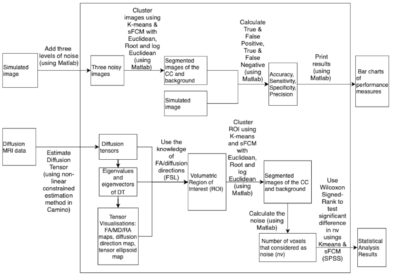
The step-by-step calculations for the following two simulation studies are summarised in a block diagram (Figure A1 in Appendix B).

3.1.1. Simulation Study 1

Tensors in the CC have small size, horizontal diffusion direction (i.e., the water diffuses between right and left hemisphere of the brain) and high FA. Regions nearby to the CC consist of other white matter (WM) tissues, grey matter (GM) and cerebrospinal fluid (CSF). Tensors in some WM regions have similar sizes and FA to that of the CC, whilst tensors in GM and CSF have larger sizes and smaller FA than that of the CC (since the diffusion is anisotropic in WM and isotropic in GM and CSF). Therefore, tensors are initially simulated from multiple regions, mimicking a real brain image, with differing FA and sizes of tensors around the CC (see Figure 1a).
Then, three levels of noise s d ( ( X j ) l s ) = 0.3 × 10 5 (noise1a), s d ( ( X j ) l s ) = 0.4 × 10 5 (noise2a) and s d ( ( X j ) l s ) = 0.5 × 10 5 (noise3a) are added to the simulated (original) region (see Figure 1b–d). The signal-to-noise ratios (SNR) of the three level of noises are 21, 18, and 15. The results of segmentation of the three noisy regions are shown in Figure 2. The figures visibly demonstrate that sFCM improved the segmentation by reducing the background noise as compared to K-means.
To provide more detailed comparisons, all of the performance measures considered for the six cases are shown in Figure 3. It can be seen that sCFM with each metric (Euclidean, log Euclidean, and root Euclidean) almost always outperformed K-means with the same metric for all performances measures; the only exceptions are the equality of sensitivity for log Euclidean at noise level 3a, and both root and log Euclidean at noise level 1a.
Furthermore, sCFM with root Euclidean or log Euclidean generally outperform sCFM with Euclidean. In detail: (i) at noise level 1a, root and log Euclidean produce the same results, and thus yield equality for all performance measures, and their measures all outperform Euclidean except for the (equality of) sensitivity; (ii) at noise levels 2a and 3a, root Euclidean has the highest accuracy, sensitivity, F-measure, and Gmean, whilst log Euclidean has the highest specificity and precision. Euclidean has the lowest values for accuracy, F-measure, specificity, and precision, but the same sensitivity as root Euclidean, and a higher Gmean than log Euclidean.

3.1.2. Simulation Study 2

In Simulation Study 1, multiple regions with increasing noise levels were used, which covers a low to moderate range of noise (since the detection of the regions becomes problematic when considering high levels of noise). In Simulation Study 2, consideration of robustness in the face of moderate to high levels of noise is enabled by simulating a homogenous region of the CC and a background only (as per the logical image mentioned earlier); this is because the CC is still visible in this case.
Initial tensors are simulated such that: the tensors have the same determinants (sizes), FA values, and eigenvalues, and they only differ in their orientation (i.e., the eigenvectors); the diffusion directions of the tensors in the simulated CC shape are parallel to y-axis, while the diffusion directions of other tensors are parallel to x-axis. Then, the three levels of noise chosen are: s d ( ( X j ) l s ) = 0.5 × 10 5 (noise1b), s d ( ( X j ) l s ) = 0.75 × 10 5 (noise2b), and s d ( ( X j ) l s ) = 0.1 × 10 4 (noise3b).
These are added to the simulated region (see Figure 4). The signal-to-noise ratio (SNR) of the three levels of noise are 13, 8, and 5. The results of the segmentation of the three noisy images are shown in Figure 5. When using Log Euclidean with noise3b (in Figure 5c), the CC is not visible. The performance measures were calculated and are shown in Figure 6. Similar to Simulation Study 1, it can be seen that root Euclidean generally provided the highest values of performance measures as compared to the other methods.
The findings indicated that: (i) at noise level 1b, all of the six methods yield the same results; (ii) at noise level 2b, sFCM yields the same results using log, root, and Euclidean (and hence the same values of all performance measures), whilst sFCM with each metric almost always outperforms K-means with the same metric (with exceptions that sFCM and K-means with the Euclidean metric have the same specificity and precision, and sFCM and K-means with root Euclidean have the same sensitivity); (iii) at noise level 3b, the log Euclidean metric fails to even detect the CC, whilst sFCM with root Euclidean outperforms sFCM with Euclidean, and sFCM with either metric (root or Euclidean) outperforms K-means with the same metric.
From both studies, it can be seen that the sFCM method improved the segmentation of the CC, almost always providing better performance measures than the corresponding K-means method, especially in noisy images. One can observe that root Euclidean with sFCM almost always outperformed Euclidean and log Euclidean in the segmentation of the CC. With the largest level of noise (i.e., noise3b in Study 2), log Euclidean failed to even detect the shape of CC even when the cluster size was increased. This is likely to be because it is highly affected by outliers, as shown by the following example.
Take three examples of tensors D 1 , D 2 , and D 3 from the CC region of a healthy brain, as follows:
D 1 = 10 8 × 0.1461 0.0329 0.0012 0.0329 0.0098 0.0066 0.0012 0.0066 0.0170
D 2 = 10 8 × 0.1683 0.0031 0.0226 0.0031 0.0169 0.0025 0.0226 0.0025 0.0070
D 3 = 10 8 × 0.1152 0.0669 0.0032 0.0669 0.0542 0.0118 0.0032 0.0118 0.0140
To calculate the log and root Euclidean distances between these tensors, the eigenvalues λ 1 , λ 2 and λ 3 of each tensor are needed (see Table 1 and Appendix A). The eigenvalues, together with the FA values are shown in Table 3, and then the distances between the tensors are shown in Table 4.
The distances between D 1 and D 2 , and D 1 and D 3 using log Euclidean are very large in comparison with the distance between D 2 and D 3 . This is due to the use of the log function and the smaller eigenvalue 0.000028 of D 1 in comparison with the other eigenvalues. All three tensors have high FA (see Table 3; recall FA ranges from 0 to 1), and hence all of them are expected to be part of the CC. When clustering, all the three tensors are part of the CC using the root Euclidean and Euclidean metrics, but D 1 is excluded from the CC using the log Euclidean metric. This explains the holes in the CC that appear using the log Euclidean metric. This example demonstrates that the distance between tensors with similar FA values can be very large when using the log Euclidean metric.

3.2. Real Brain Image Data Studies

In this section, the application in practice, using real brain image data, is considered, demonstrating that sCFM performs significantly better than K-means for the segmentation of the CC. Subsequently, using the same data set, a brief demonstration that the methods can be used effectively for classification as well as segmentation is provided. Furthermore, it is demonstrated (using sFCM, which ensures robustness to noise) that existing DTI indices (fractional anisotropy, mean diffusivity, and radial diffusivity), as well as the determinant, are all suitable DTI indexes that can be used to distinguish between healthy and SCA2 subjects and are sensitive to ageing effects.
The data consists of nine SCA2 subjects (six males and three females) and sixteen age-matched healthy subjects (nine males and seven females). This data is taken from [23]. On the same MRI scanner, the subjects have been imaged twice: 3.6 ± 0.7 years apart (SCA2 patients) and 3.3 ± 1.0 years apart (control subjects). For more details about the data and MRI acquisition procedures see [23]. In this work, diffusion weighted data is corrected for eddy current-induced distortions (using FSL). Then, the diffusion tensor imaging is fitted using a non-linear constrained estimation method [24,25] in Camino. Matlab and SPSS are used for segmentation and data analysis respectively. The block diagram of the calculations is presented in Figure A1 in Appendix B.

3.2.1. 3D Segmentation of the CC

A volumetric region of interest (ROI) from the middle of the brain is chosen as input to the K-means and sFCM (with parameters used p = 2 and q = 1.5 ) algorithms. The ROI is clustered into five clusters, with CC being one of those clusters, using the root Euclidean metric. To visualise the CC, the cluster labels are binarised (i.e., cluster labels for the CC cluster are all 1 and 0 is used for labels in the other four clusters). Examples of the results of the segmentation of the CC using K-means and sFCM are shown in Figure 7. To evaluate how much better sFCM is in reducing the noise around the CC as compared to K-means, the number of voxels (nv) that are considered as noise is calculated (i.e., the voxels around the CC that have the same cluster labels as the CC but are not actually part of the CC).
The Wilcoxon Signed-Rank test is used to test the significant difference in nv values produced by using K-means and sFCM. The results show that the nv values are significantly smaller using sFCM as compared to K-means (see Table 5) for both the baseline and post baseline data. This confirms that the use of sFCM instead of K-means significantly reduced the amount of noise in these images.

3.2.2. Generalisation to Classification of Brain Images

These new methods can be used for the more general problem of classifying a brain image into white matter, grey matter, and cerebrospinal fluid, using a whole axial slice of the brain image. Since the image contains both the brain and its background, the image is clustered into four clusters for white matter, grey matter, cerebrospinal fluid, and the background of brain (see Figure 8, where the background is shown in deep blue) using the root Euclidean metric. The CC is not segmented here, but is included as part of the white matter. To segment the CC, the cluster size needs to be 5 (as in Section 3.2.1); however, this demonstrates that sFCM can be used for classification purposes.

3.2.3. Clinical Applications of Segmentations with sFCM

In clinical studies, DTI indices, such as Fractional anisotropy (FA), mean diffusivity (MD), and Radial diffusivity (RD), are used in the comparison of healthy and non-healthy brain images (often manually segmented). The efficacy of the new methods presented in the paper is demonstrated by using one of our automatically created segmentations (via sFCM with root Euclidean) and demonstrating that these indices can distinguish between healthy and SCA2 subjects, and they are sensitive to ageing effects.
This reaffirms the results in the literature [12,13,15], but with the extra knowledge that the use of sFCM will have reduced the impact of noise. In addition to this, it can be seen that the determinant (DET) of the tensors, which is easy to compute, can also be used to distinguish between healthy and SCA2 subjects and is sensitive to ageing effects. That is, DET is shown to be a viable DTI index.
First, recall the definitions of the DTI indices, which are functions of the eigenvalues of the diffusion tensors. FA measures the deviations from isotropic diffusion of water inside a voxel in the brain, and it is a fraction with FA equal to 1 for diffusion that is highly anisotropic (i.e., water diffuses in one direction) and FA equal to 0 for isotropic diffusion (i.e., water diffuses in all directions). Let λ 1 , λ 2 and λ 3 be the eigenvalues of diffusion tensor D and assume that λ 1 is the largest eigenvalue. Then, FA [5] can be calculated as follows:
FA = ( λ 1 λ 2 ) 2 + ( λ 2 λ 3 ) 2 + ( λ 3 λ 1 ) 2 2 ( λ 1 2 + λ 2 2 + λ 3 2 ) .
MD measures the average water diffusivity in a voxel in the brain. It is calculated as follows [5]:
MD = λ 1 + λ 2 + λ 3 3 .
Radial diffusivity measures the perpendicular diffusion to the main diffusion of water. It is calculated as follows [5]:
RD = λ 2 + λ 3 2 .
These DTI indices, together with the DET are computed. The Mann–Whitney test is used to test the significant difference in FA, MD, RD, and DET between healthy and SCA2 subjects at the significance level 0.05. The results of FA, MD, RD, and DET are all significant at both baseline and post baseline. In detail:
  • FA values in SCA2 subjects are significantly lower than in healthy subjects (p-value at baseline = 0.0005 , p-value at post baseline = 0.0004 ).
  • MD values in SCA2 subjects are significantly increased as compared to healthy subjects (p-value at baseline = 0.018 , p-value at post baseline = 0.035 ).
  • RD values in SCA2 subjects are significantly increased as compared to healthy subjects (p-value at baseline = 0.0005 , p-value at post baseline = 0.0007 ).
  • DET values in SCA2 subjects are significantly larger than in healthy subjects (p-value at baseline = 0.001 , p-value at post baseline = 0.002 ).
These results show that FA, MD, RD, and DET distinguish well between healthy and SCA2 subjects. The rate of change can be calculated as follows:
Rate of change = data baseline data post baseline number of days in between
The rates of change of FA, MD, RD, and DET in SCA2 subjects are not significantly different from the rates of change in healthy subjects.
The Wilcoxon Signed-Rank test is used to test the significant difference in FA, MD, RD, and DET at baseline and post baseline. The results of FA, RD, and DET were all significant. However, MD values were not significantly different at baseline and post baseline. The details are as follows:
  • FA values at post baseline were significantly lower than at baseline (p-value = 0.0001 ).
  • RD values at post baseline were significantly increased as compared to RD values at baseline (p-value = 0.0004 ).
  • DET values at post baseline were significantly larger than at baseline (p-value = 0.003 ).
These results show that FA reduced while RD and size of tensors (DET) increased with age.

4. Conclusions and Discussion

Manual segmentation of the CC is often done slice by slice, and hence it is very time consuming and is also subject to intra and interobserver variability. In this paper, we presented an automatic and accurate method for segmentation of the CC that will save time and effort for radiologists by eliminating the need of manual segmentation. The method uses uncertainty information in the segmentation decisions by calculating the probabilities (membership values) of each voxel to belong to different clusters. The spatial contextual information is exploited.
We demonstrated that sFCM outperformed K-means with the same metric for segmentation of the CC and sFCM with the root Euclidean metric as the preferred option. In this paper, the method was extended to a matrix-type of data (covariance matrix data) and was used for DTI classification (to classify images into white matter, grey matter, and cerebrospinal fluid).
Further research about classification of different brain regions using this method will be carried out in future work. The CC in SCA2 subjects were compared with healthy subjects. We demonstrated that the determinant of diffusion tensors and DTI indices can be used to distinguish between SCA2 and healthy subjects and are sensitive to ageing effects. Hence, the determinant of diffusion tensors is useful for the detection of abnormalities in the CC and for surgical planning.
The non-Euclidean metrics used in sFCM were the log-Euclidean and root Euclidean metrics as their calculations are straightforward. It would be interesting to use other non-Euclidean metrics, although numerical algorithms may need to be used. For example, the Procrustes size-and-shape metric may provide new segmentation results.
A regularisation model was proposed for sFCM—currently, for the smooth part, the power parameter r 1 = 2 , and the regularisation parameter λ = 0 . For various structures in the brain, the regularisation model would still need to be carefully tuned. It would be interesting to explore segmentation results when varying the parameters in the model. An efficient way to determine the reference tensor with the expected diffusion behaviour is needed for practical users.
There are regions in the brain with more than one distinct fibre orientation captured in a single voxel. For example, two crossing fibres would need two diffusion tensors to model the diffusion behaviour at a single voxel. Tensor field segmentation becomes more challenging for the regions with crossing fibres. A basic and difficult question is how to measure the dissimilarity between a pair of tensors at one voxel and a pair of tensors at another voxel. To develop segmentation methods for DTI data containing crossing fibres is also of interest.

Author Contributions

Conceptualization, D.Z.; methodology, A.F., D.Z. and S.E.; software, S.E.; validation, A.F.; formal analysis, S.E.; investigation, S.E.; resources, A.F., D.Z. and S.E.; data curation, A.F., D.Z. and S.E.; writing—original draft preparation, S.E.; writing—review and editing, A.F., D.Z.; visualization, A.F., D.Z. and S.E.; supervision, A.F., D.Z.; project administration, D.Z.; funding acquisition, A.F. and D.Z. All authors have read and agreed to the published version of the manuscript.

Funding

This research was funded by the Higher Education Innovation Funding-UK and the EPSRC IAA (UK).

Data Availability Statement

The SCA2 image data used in this paper is freely available from [23].

Conflicts of Interest

The authors declare no conflict of interest. The funders had no role in the design of the study; in the collection, analyses, or interpretation of data; in the writing of the manuscript, or in the decision to publish the results.

Abbreviations

The following abbreviations are used in this manuscript:
DTdiffusion tensor
FCMfuzzy c-means
sFCMspatial fuzzy c-means
CCcorpus callosum
SCA2apinocerebellar ataxia 2
FAfractional anisotropy
MDmean diffusivity
RDradial diffusivity
AXaxial diffusivity
MOmode of anisotropy
WCSSwithin-cluster sum of squares
NBneighbouring voxels
TPtrue positive
TNtrue negative
FPfalse positive
FNfalse negative
WMwhite matter
GMgrey matter
CSFcerebrospinal fluid
SNRsignal-to-noise ratio

Appendix A. Background Definitions

The spectral decomposition of a symmetric positive definite matrix A is given by A = V Λ V where V is an orthonormal matrix and Λ is diagonal matrix of eigenvalues as follows:
V = v 1 v g
Λ = λ 1 0 0 0 λ 2 0 0 0 λ g
where λ i 0 , for i 1 , , g . Then, A to the power k, where k R , is obtained by:
A k = V Λ k V .
The exponential of A can be obtained by:
exp ( A ) = V exp ( Λ ) V .
The logarithm of A is given by:
log ( A ) = V log ( Λ ) V
where Λ entries are strictly positive eigen values.
Cholesky decomposition (factorization) of the positive semi-definite matrix A is given by A = L L T where L is a lower triangular matrix with nonnegative diagonal elements as follows:
L = chol ( A ) = a 11 0 0 a 21 a 22 0 0 a g 1 a g 2 a g g
where a i i 0 , for i = 1 g . Cholesky factorization is unique for positive definite matrices with a i i > 0 .

Appendix B. Block Diagrams for Simulation Studies and Real Data Applications

Figure A1. Block diagram for simulation studies and real data applications.
Applsci 11 07003 g0a1

References

  1. Hardan, A.; Minshew, N.; Keshavan, M. Corpus callosum size in autism. Neurology 2000, 55, 1033–1036. [Google Scholar] [CrossRef]
  2. Downhill, J.E., Jr.; Buchsbaum, M.S.; Wei, T.; Spiegel-Cohen, J.; Hazlett, E.A.; Haznedar, M.M.; Silverman, J.; Siever, L.J. Shape and size of the corpus callosum in schizophrenia and schizotypal personality disorder. Schizophr. Res. 2000, 42, 193–208. [Google Scholar] [CrossRef]
  3. Walterfang, M.; Fahey, M.; Abel, L.; Fietz, M.; Wood, A.; Bowman, E.; Reutens, D.; Velakoulis, D. Size and shape of the corpus callosum in adult Niemann-Pick type C reflects state and trait illness variables. Am. J. Neuroradiol. 2011, 32, 1340–1346. [Google Scholar] [CrossRef] [Green Version]
  4. Basser, P.J.; Jones, D.K. Diffusion-tensor MRI: Theory, experimental design and data analysis–a technical review. NMR Biomed. Int. J. Devoted Dev. Appl. Magn. Reson. Vivo 2002, 15, 456–467. [Google Scholar] [CrossRef] [Green Version]
  5. Le Bihan, D.; Mangin, J.F.; Poupon, C.; Clark, C.A.; Pappata, S.; Molko, N.; Chabriat, H. Diffusion tensor imaging: Concepts and applications. J. Magn. Reson. Imaging Off. J. Int. Soc. Magn. Reson. Med. 2001, 13, 534–546. [Google Scholar] [CrossRef]
  6. Dryden, I.L.; Koloydenko, A.; Zhou, D. Non-Euclidean statistics for covariance matrices, with applications to diffusion tensor imaging. Ann. Appl. Stat. 2009, 3, 1102–1123. [Google Scholar] [CrossRef] [Green Version]
  7. Zhou, D.; Dryden, I.L.; Koloydenko, A.A.; Audenaert, K.M.; Bai, L. Regularisation, interpolation and visualisation of diffusion tensor images using non-Euclidean statistics. J. Appl. Stat. 2016, 43, 943–978. [Google Scholar] [CrossRef] [Green Version]
  8. Ge, Y.; Law, M.; Johnson, G.; Herbert, J.; Babb, J.S.; Mannon, L.J.; Grossman, R.I. Preferential occult injury of corpus callosum in multiple sclerosis measured by diffusion tensor imaging. J. Magn. Reson. Imaging Off. J. Int. Soc. Magn. Reson. Med. 2004, 20, 1–7. [Google Scholar] [CrossRef]
  9. Gupta, R.K.; Saksena, S.; Hasan, K.M.; Agarwal, A.; Haris, M.; Pandey, C.M.; Narayana, P.A. Focal Wallerian degeneration of the corpus callosum in large middle cerebral artery stroke: Serial diffusion tensor imaging. J. Magn. Reson. Imaging Off. J. Int. Soc. Magn. Reson. Med. 2006, 24, 549–555. [Google Scholar] [CrossRef] [PubMed]
  10. Kubicki, M.; Styner, M.; Bouix, S.; Gerig, G.; Markant, D.; Smith, K.; Kikinis, R.; McCarley, R.W.; Shenton, M.E. Reduced interhemispheric connectivity in schizophrenia-tractography based segmentation of the corpus callosum. Schizophr. Res. 2008, 106, 125–131. [Google Scholar] [CrossRef] [PubMed] [Green Version]
  11. Schöls, L.; Bauer, P.; Schmidt, T.; Schulte, T.; Riess, O. Autosomal dominant cerebellar ataxias: Clinical features, genetics, and pathogenesis. Lancet Neurol. 2004, 3, 291–304. [Google Scholar] [CrossRef]
  12. Mandelli, M.L.; De Simone, T.; Minati, L.; Bruzzone, M.; Mariotti, C.; Fancellu, R.; Savoiardo, M.; Grisoli, M. Diffusion tensor imaging of spinocerebellar ataxias types 1 and 2. Am. J. Neuroradiol. 2007, 28, 1996–2000. [Google Scholar] [CrossRef] [Green Version]
  13. Hernandez-Castillo, C.R.; Galvez, V.; Mercadillo, R.; Diaz, R.; Campos-Romo, A.; Fernandez-Ruiz, J. Extensive white matter alterations and its correlations with ataxia severity in SCA2 patients. PLoS ONE 2015, 10, e0135449. [Google Scholar] [CrossRef]
  14. Mascalchi, M.; Toschi, N.; Giannelli, M.; Ginestroni, A.; Della Nave, R.; Nicolai, E.; Bianchi, A.; Tessa, C.; Salvatore, E.; Aiello, M.; et al. Progression of microstructural damage in spinocerebellar ataxia type 2: A longitudinal DTI study. Am. J. Neuroradiol. 2015, 36, 1096–1101. [Google Scholar] [CrossRef] [Green Version]
  15. Mascalchi, M.; Marzi, C.; Giannelli, M.; Ciulli, S.; Bianchi, A.; Ginestroni, A.; Tessa, C.; Nicolai, E.; Aiello, M.; Salvatore, E.; et al. Histogram analysis of DTI-derived indices reveals pontocerebellar degeneration and its progression in SCA2. PLoS ONE 2018, 13, e0200258. [Google Scholar] [CrossRef]
  16. Chuang, K.S.; Tzeng, H.L.; Chen, S.; Wu, J.; Chen, T.J. Fuzzy c-means clustering with spatial information for image segmentation. Comput. Med Imaging Graph. 2006, 30, 9–15. [Google Scholar] [CrossRef] [Green Version]
  17. Elsheikh, S.; Fish, A.; Chakrabarti, R.; Zhou, D. Cluster Analysis of Diffusion Tensor Fields with Application to the Segmentation of the Corpus Callosum. Procedia Comput. Sci. 2016, 90, 15–21. [Google Scholar] [CrossRef] [Green Version]
  18. Arsigny, V.; Fillard, P.; Pennec, X.; Ayache, N. Log-Euclidean metrics for fast and simple calculus on diffusion tensors. Magn. Reson. Med. Off. J. Int. Soc. Magn. Reson. Med. 2006, 56, 411–421. [Google Scholar] [CrossRef]
  19. Bezdek, J.C. Pattern Recognition with Fuzzy Objective Function Algorithms; Springer Science & Business Media: Boston, MA, USA, 2013. [Google Scholar]
  20. Wang, Z.; Vemuri, B.C. DTI segmentation using an information theoretic tensor dissimilarity measure. IEEE Trans. Med. Imaging 2005, 24, 1267–1277. [Google Scholar] [CrossRef]
  21. Lenglet, C.; Rousson, M.; Deriche, R. Segmentation of 3D probability density fields by surface evolution: Application to diffusion MRI. In Proceedings of the International Conference on Medical Image Computing and Computer-Assisted Intervention, Saint-Malo, France, 26–29 September 2004; pp. 18–25. [Google Scholar]
  22. Bekkar, M.; Djemaa, H.K.; Alitouche, T.A. Evaluation measures for models assessment over imbalanced data sets. J. Inf. Eng. Appl. 2013, 3, 27–38. [Google Scholar]
  23. Openneuro.org. Stanford Center for Reproducible Neuroscience. Available online: https://openneuro.org/datasets/ds001378/versions/00003 (accessed on 1 November 2019).
  24. Jones, D.K.; Basser, P.J. “Squashing peanuts and smashing pumpkins”: How noise distorts diffusion-weighted MR data. Magn. Reson. Med. Off. J. Int. Soc. Magn. Reson. Med. 2004, 52, 979–993. [Google Scholar] [CrossRef] [PubMed]
  25. Alexander, D.C.; Barker, G.J. Optimal imaging parameters for fiber-orientation estimation in diffusion MRI. Neuroimage 2005, 27, 357–367. [Google Scholar] [CrossRef] [PubMed]
Figure 1. The original tensors in comparison with the tensors having added the three levels of noise.
Applsci 11 07003 g001
Figure 2. Segmentation after adding three levels of noises.
Applsci 11 07003 g002
Figure 3. Bar charts of the performance measures for Simulation Study 1. Overall, sFCM yields higher values of performance measures as compared to K-means, whilst root Euclidean yields the highest performance measures. To enable better visualisation of the results, a scale of 45–100 for precision and F-measure and 80–100 for the rest of the measures is used.
Applsci 11 07003 g003
Figure 4. Original and noisy tensors before and after adding three levels of noise.
Applsci 11 07003 g004
Figure 5. Segmentation after adding three levels of noises.
Applsci 11 07003 g005
Figure 6. Bar charts of the performance measures. Root Euclidean using sFCM generally yields the highest values of performance measures. Using log Euclidean, the CC is not even detectable at noise level 3b (denoted here by a *). To enable better visualisation of the results, a scale of 45–100 for precision and F-measure and 80–100 for the rest of the measures is used.
Applsci 11 07003 g006
Figure 7. Segmentation of the CC for healthy and SCA2 brain images using K-means and sFCM.
Applsci 11 07003 g007
Figure 8. Classification of brain into white matter (green), grey matter (yellow), and cerebrospinal fluid (blue).
Applsci 11 07003 g008
Table 1. Distance D ( A j , A ¯ i ) using the Euclidean, log, and root Euclidean.
MetricDistance
Euclidean A j A ¯ i
Log Euclidean log ( A j ) log ( A ¯ i )
Root Euclidean A j 1 / 2 A ¯ i 1 / 2
Table 2. Weighted mean A ¯ using the Euclidean, log, and root Euclidean.
MetricMean
Euclidean i = 1 n w i j m A j i = 1 n w i j m
Log Euclidean exp i = 1 n w i j m log A i i = 1 n w i j m
Root Euclidean i = 1 n w i j m A i 1 / 2 i = 1 n w i j m i = 1 n w i j m A i 1 / 2 i = 1 n w i j m
Table 3. Eigenvalues of D 1 , D 2 , and D 3 ( × 10 8 ) .
Tensor λ 1 λ 2 λ 3 FA
D 1 0.15370.01920.0000280.936
D 2 0.17140.01710.00360.937
D 3 0.15880.02060.00400.919
Table 4. The distances between the tensors.
MethodDist ( D 1 , D 2 )Dist ( D 1 , D 3 )Dist ( D 2 , D 3 )
Euclidean3.3689 ×   10 19 2.2948 ×   10 18 1.5564 ×   10 18
Log Euclidean42.168151.41215.9165
Root Euclidean1.2426 ×   10 9 4.7398 ×   10 9 2.3534 ×   10 9
Table 5. Mean and standard deviation (Std) of nv.
MethodMean (nv)Std (nv)p-Value
K-means (baseline)18.869619.4593.0.00004
sFCM (baseline)2.95654.1939
K-means (post)31.652265.72850.00004
sFCM (post)3.60875.6387
Publisher’s Note: MDPI stays neutral with regard to jurisdictional claims in published maps and institutional affiliations.

