Minimizing the Total Weighted Waiting Times and Instability in a Rescheduling Problem with Dynamic Jobs Weight

Abstract

Thanks to smart technological tools, customers can at any moment create or modify their commands. This reality forced many production firms to become sensitive in rescheduling processes. In the literature, most of rescheduling problems consider classical efficiency measures. However, some existing works also consider stability as a measure for limiting the deviation from initial schedule. In this work, we aim to bridge the gap in existing works on rescheduling by investigating a new approach to measure simultaneously efficiency by the total weighted waiting times and stability by the total weighted completion time deviation. This combination of criteria is very significant in industrial and hospital environments. In this paper, a single machine rescheduling problem with jobs arriving over time is considered. A mixed integer linear programming (MILP) model is designed for this problem and an iterative predictive-reactive strategy for dealing with the online part. Numerical results show that, at each time the jobs are rescheduled, the low weight ones move forward. Consequently, a new concept consisting in increasing the jobs weight as function of time is established. The effect of this new conception is evaluated by the variation of the average flowtime. Eventually, the computing time of the MILP resolution is studied to explore its limitations.

1. Introduction

Through new technologies development, today’s industry is currently experiencing the 4th revolution, referred to as Industry 4.0. This reality has a significant impact on the industrial management processes [1,2,3]. Hence, the customers practices are changed, they can, at any moment, create or modify their commands through new technological tools, such as the laptop, the tablet computer, or the smart phone [4,5]. Indeed, these situations have an impact on the production scheduling [6,7]. In addition, production problems can also disrupt the already established sequence, for instance, the mechanical machine breakdowns, or the lack of raw materials, etc. These factors force many production firms to react for updating the existing schedule. Hence, the rescheduling is necessary to revise schedules in a cost-effective manner [8].

Rescheduling is the mechanism of updating an established production schedule as a response to disruptions [8]. Many types of disruptions have been studied, such as the arrival of new jobs [9,10], machine breakdowns [11,12,13], operational unit failures [14], job rejection [15], quality problems and shortage of raw materials [16,17]. Over the last few years, many researches dealt with this area and dedicated to it more attention. Indeed, rescheduling studies have considered many types of machine environments [18,19,20,21].

The classical efficiency criteria are often used for measuring the performance of the schedule, such as the Makespan [22,23,24,25], Makespan combined with tardiness [26], total completion times [27,28], total weighted completion times [29,30], total weighted tardiness [31], total tardiness [32], total flow time [33] and maximum lateness [34]. Different from existing works, this one investigates new performance measures. In terms of efficiency, the Total Weighted Waiting Times (TWWT) is considered as a criterion. The waiting time represents the duration that the job has waited in the system before being executed [35]. In some real-life environments, the TWWT is a very significant criterion. For instance, in production systems, it can represent the waiting time of a job in front of a workstation, considering the importance of the job as a weight. In the operating rooms scheduling, it represents the delay between the patient’s arrival and the starting time of his treatment, considering the patient emergency level as a weight. In Guo et al., the authors addressed a problem of rescheduling the jobs considering as an objective the maximum waiting time. The problem is inspired from quartz manufacturing industry. In which the waiting time is considered as the waiting for certain materials in oven before the reheating step, where both the rework flow and the regular production flows meet [36]. Thus, the authors studied and analyzed the complexity of a rescheduling problem on a single machine, to decide where to insert the rework jobs in the initial sequence of regular jobs, to minimize the maximum waiting time. Guo and Xie considered a problem of the total waiting time minimization on a single machine rescheduling environment. The authors formulated two mixed integer programming models [37]. The studied problem is also an illustration of quartz glass factory, where the waiting time represents the waiting of materials before the welding step. The minimization of the waits saves the energy consumption. In our study, the TWWT is considered as a criterion. This criterion has been discussed for the first time by Rinnooy Kan, in 1976 [38].

Even if the efficiency measures the performance of a scheduling system, it is not the only measure for dynamic rescheduling problems. Stability measure, limiting the deviation from the initial schedule is also studied in the literature [39,40,41]. During rescheduling event, this measure evaluates the impact of the movement of the jobs [42]. In real life applications, the changes of the sequence may generate supplementary costs, such as raw materials reordering costs and reallocation costs [43,44,45,46,47,48,49,50]. In this work, a new stability criterion is studied, it consists in measuring the difference between the sum of completion times of the jobs in the initial schedule and in the new one, assigning to each job a weight, referred to as the total weighted completion time deviation (TWCTD). The weights association makes difficult to disrupt the jobs with high weights. This is the case of an urgent patient in a hospital, for example.

Vieira et al. [8] and Herrmann [51] distinguished two basic rescheduling strategies. The first strategy is completely reactive, it is often referred to as dynamic scheduling strategy. In this strategy, the schedule is dynamically constructed by dispatching jobs when it is necessary. It uses locally the available information to decide which job to execute. Therefore, dispatching rules or other heuristics are used to prioritize jobs waiting to be processed on the machine [52,53]. The second is the predictive~-reactive rescheduling strategy, it consists in firstly generate an initial schedule and to update secondly this schedule, at each time a disruption occurs [54,55,56,57]. In our approach, the predictive–reactive rescheduling strategy is also adopted through firstly solving an initial problem with the objective of minimizing the TWWT. After the occurrence of a disruption, the objective becomes to minimize a new criterion combining simultaneously the schedule efficiency and the schedule stability, with the TWCTD as a stability measure. As in the majority of the rescheduling problems considering the efficiency and the stability [58,59], a relationship between both objective is established, by associating a coefficient for each measure (i.e., α efficiency + (1 − α) stability), referred to as the efficiency-stability coefficient. The influence of this coefficient on the system is later discussed. Considering simultaneously the schedule efficiency and schedule stability in the second objective function, plays a more significant role for reducing the actual costs in real applications. In the literature, some classical single machine scheduling models, uses rescheduling assumption to determine new schedules in response to disruptions. These previous models are only based on the classical measures Thus, several costs are disregard. Along with that, based on the numerical results observation, a new concept consisting in increasing the weight in function of time is introduced. This concept allows to avoid ignoring the jobs with low weights thanks to increasing their weights in function of time. The weight increasing effect is also discussed in the numerical results section.

This work investigates a single machine rescheduling problem, the disruptions are caused by new jobs arrival. The choice of the single machine environment is motivated by the fact that this environment represents several real-life cases, for example a single operating room in a hospital or a single workstation in a factory. Moreover, according to Pinedo, the single machine provides a basis for heuristics that are applicable to more complicated machine environments [60]. In practice, scheduling problems in more complicated machine environments are often decomposed into sub-problems that deal with single machines. Thus, a mixed integer linear programming model is implemented to describe this problem and an iterative methodology is proposed for dealing with the online part. This work is a contribution to operational research area. The main research objectives are:

-

Considering simultaneously the TWWT as the schedule efficiency and the TWCTD as the schedule stability. These two criteria are mixed in one performance measure.

-

Implementing for this specific problem, a mathematical model based on the MILP and an iterative predictive-reactive methodology for solving the online problem. In addition, testing the limitation of the MILP resolution in terms of number of jobs.

-

Establishing an innovative concept that consists in varying the jobs weight in function of time spent in the system, thus helping the low-weighted earliest operations to be executed.

The rest of paper is organized as follows. In Section 2, the literature review is discussed. In Section 3, we motivate our research work. The problem and the proposed methodology are described in Section 4. The mathematical model is then presented in Section 5. The numerical results are analyzed in Section 6. Finally, conclusions and perspectives are given in Section 7.

2. Literature Review

This section is dedicated to the literature review of rescheduling problem. Rescheduling literature is very rich. At those time, Vieira et al. [8], Ouelhadj and Petrovic [61] and, recently, Uhlmann and Frazzon [62], provided a detailed reviews on rescheduling problems. Indeed, rescheduling studies have considered many types of machine environments. For example, Da Silva et al. considered a dynamic rescheduling problem where the set of original jobs has been scheduled on a single machine when new customer orders arrive, requiring the execution of a new job or the cancellation of previously ordered one [18]. The authors proposed an approach that reconsiders the actual schedule, at each time a new event arrives. A mixed integer linear programming model is formulated with the aim of minimizing the Makespan. Angel-Bello et al. recently studied the makespan minimization in a single machine rescheduling problem with jobs arrival as a disruption [19]. The authors implemented two rescheduling strategies. The first one uses all the available jobs at the rescheduling point to obtain an optimal solution. The second one considers only the jobs that can be completed until the next re-optimization point. Alagöz and Azizoğlu studied, under machine eligibility constraints, a rescheduling problem in parallel machine environments [20]. The total flow time is considered as an efficiency criterion and the number of jobs that change the machine after rescheduling as stability criterion. The authors proposed several heuristics to provide approximate solutions. Gao et al. studied a flexible job shop rescheduling problem with new job insertion [21]. The authors considered multiple objectives to measure the performance of rescheduling: Makespan, average of earliness and tardiness, maximum machine workload and total machine workload. Four sets of heuristics are proposed for this problem and their effectiveness are studied. Most of these works, consider the classical efficiency criteria for measuring the performance of the schedule, such as the Makespan [22,23,24,25], Makespan combined with tardiness [26], total completion times [27,28], total tardiness [32], total flow time [33] and maximum lateness [34]. The majority of these criteria only consider the processing times to construct the schedule. In real applications, when new orders arrive, the priorities of these orders are also taken into account, such as, the customers priorities in the industrial manufacturing or the emergency levels in the operating room rescheduling. Some operations, despite their short duration, are more important than others since their high priorities or emergency levels. Therefore, it seems unrealistic to delay the short duration operations to insert new operations, only based on the durations. Thus, the TWWT is considered as an efficiency criterion on this work.

Even if the efficiency measures the performance of a scheduling system, it is not the only measure for dynamic rescheduling problems. Stability measure, limiting the deviation from the initial schedule is also studied in the literature. For instance, Akkan studied in 2015 a rescheduling problem considering simultaneously the schedule efficiency measured with the maximum tardiness and the schedule stability measured with the sum of absolute starting time deviations. This stability criterion calculates the sum of absolute difference between the jobs starting times before and after rescheduling [44]. The author proved that their algorithm improves the schedule stability without impacting T_max. Liu and Zhou studied a rescheduling problem on identical parallel machines and considered two conflicting rescheduling criteria: the total completion time as a measure of scheduling cost efficiency and the number of jobs assigned to different machines in the original schedule and newly generated schedule as a measure of stability cost [28]. Rahmani and Ramezanian considered a dynamic flexible flow shop scheduling that simultaneously measured the schedule efficiency by the total weighted tardiness and the schedule stability by the absolute deviation of completion times [43]. The considered stability criterion measures the difference between the completion time of the jobs before and after the rescheduling. Indeed, when the sequence is disrupted, the initial jobs completion times may change and will be replaced by real completion times obtained after the rescheduling. Moreover, there are also several works dealing with the stability measure in the rescheduling problems, such as the starting time deviation and the total deviation penalty [42], the starting time deviation [45], the amount of operations and the starting times operations have been altered [46], the absolute positional disruption, the positional disruption and the absolute completion time disruption [47], the total sequence disruption [48], the maximum time disruption (change of delivery times of jobs to customers) [49] and the rescheduling cost [50]. Most of these works consider the starting or the completion time deviation as a criterion to evaluate the schedule instability. However, the movement of the important orders is not considered in these stability measures. Assigning the weights to the stability criterion, penalizes more largely the movements of the important or the urgent operations. Thus, it will be difficult to change the position of the high priority operations. To the best of our knowledge, there is only few papers that consider the weights on the stability measures. To bridge the gap, this work investigates a new stability measure by considering the TWCTD as a stability criterion.

The predictive-reactive rescheduling strategy is the most used strategy to reschedule the jobs in response to disruptions [61]. The principle of this strategy is based on two steps. The first one is the predictive step. It consists in creating an initial schedule. The second one is the reactive step. It consists of revising the established schedule, at each time, a disruption occurs, in order to minimize its impact on the schedule performance [8]. Several researchers in the literature have adopted this strategy. For instance, Bahroun et al. recently implemented in a single machine rescheduling problem, a proactive–reactive strategy consisting in the first phase to use tentative information (release dates, processing times and due dates) to construct a set of feasible schedules [63]. Then, In the second reactive phase, the schedule is progressively built as the horizon rolls forward. Yang and Geunes treated a single machine rescheduling problem where they used a predictive–reactive strategy to handle the occurrence of uncertain future jobs. Their strategy consists to determine the amount of planned idle time for uncertain future jobs and their positions as a predictive step [64]. Then, when a disruption occurs, the schedule reacts through including the new jobs in the idle time. Wang et al. treated a predictive-reactive approach of surgery scheduling problem for a single surgical suite, subject to random emergency surgeries [65]. The authors generated a primary schedule to optimize the schedule efficiency. Then, a slack time is inserted to introduce an emergency surgery when it occurs. In this work, we have used Predictive-reactive rescheduling strategy but acting differently from previous works. Firstly, we solve an initial problem with the objective of minimizing the TWWT. After occurrence of a disruption, the objective becomes to minimize a new criterion combining simultaneously the schedule efficiency and the schedule stability, with the TWCTD as a stability measure. In addition, we have associated these two criteria by a coefficient α, for helping the decision maker to find an overhead between the two problem aspects.

Several authors have opted to model the problems of operating room rescheduling as machine rescheduling problems. For example, Stuart and Kozan studied a rescheduling problem of a day-to-day running of a day surgery unit. The authors have modeled their problem as a single machine scheduling problem, considering that the sequence-dependent processing time and due date [66]. They developed a branch and bound method to tackle the problem. Wang et al. addressed, in single surgical suite, a surgery scheduling problem, where each patient should be sequenced in the same order on three stages [65]. The authors considered the arrival of random emergency surgeries as a disruption. They modeled their system as a problem of no-wait permutation flow shop scheduling and designed a predictive reactive strategy to handle the system disruption. Our research motivation is also an inspiration of the operating room rescheduling case. In the following section, we briefly present our motivation.

3. Motivation

This research is inspired by real life systems. We have taken the motivation from hospital system situation. In following paragraph, we present an illustration of this situation.

The operating theater (OT) constitutes the largest hospital cost category by 33% among the hospital departments [67,68]. Therefore, operating room scheduling has been identified as a major challenge by hospital decision-makers. In addition, according to Cardoen et al., the long waiting lists are the most received heard complaints in the health services [69]. Thus, the minimization of the patient waiting time is so interesting research area. By acting on this issue, we can improve the patient satisfaction and reduce the hospital costs. In fact, two types of operations are distinguished. The first is the elective operations when all the information are already known in advance. The second is the emergency operations which can occur at any time due to the urgent patients’ arrival. These ones are uncertain and they are considered as a disruption for the already established schedule. On the other hand, the problem of a single operating room is usually studied in the literature since it can be extended to more complicated machine environment [60]. For example, Denton et al. studied a stochastic optimization model for daily of a single operating room scheduling, then the authors extended their study in two stage stochastic resource [70]. This justifies the fact that we have modeled the problem as a single machine rescheduling problem. In addition, the patients’ categories can be divided into five major groups according to their surgery priorities [71]. Thus, it is assumed for each job a weight representing its emergency level. In this study, the objective is to model the described practical example as a problem of a single machine rescheduling. We proceed in two phases. In the predictive phase (elective), the aim is to minimize the patient weighted waiting times as an efficiency criterion. Then, in the reactive phase (emergency), the aim is to minimize the efficiency criterion combined with a stability criterion, to reduce the deviation from the initial schedule. To the best of our knowledge, in the literature, there is not any contribution dealing with this practical example and simultaneously taking into account the two previous criteria. This described system can also be encountered in industrial system, as presented in [36], considering the waiting time as the waiting of materials before the reheating step in the oven and the arrival of new orders as a disruption. The weights can also be added for representing the customer priorities.

4. Problem Description and Strategy

4.1. Problem Description

In this paper, we study a single machine rescheduling problem with disruptions caused by the arrival of new jobs. The considered problem is solved in two phases. The phase before the disruptions concerns the TWWT minimization in a static single machine scheduling problem. The second phase aims to minimize, after each disruption, simultaneously, the TWWT of jobs and the TWCTD of uninitiated jobs. In the considered problem, for each job j is associated a weight w_j, a release date r_j and a processing time p_j. When the processing of a job j starts, it is processed without preemption to completion time C_j. In this phase of the problem (predictive phase), all the job information (p_j, r_j, w_j) is known in advance. Thus, the waiting time W_j of job j is defined as W_j = C_j − p_j − r_j (see Figure 1).

Efficiency criterion: The waiting time represents the period that the job waits, from its release date r_j, until the execution at the starting time S_j, i.e., W_j = S_j − r_j. Thus, W_j = C_j − p_j − r_j, knowing that S_j = C_j − p_j (see Figure 1).

In this system, it is supposed that N = {1, 2, …, n} is a set of jobs, which are already available for scheduling at the time t = 0. In the predictive phase, the objective is to determine an initial schedule with the objective of minimizing the Total Weighted Waiting Times, i.e., ${\displaystyle {\sum }_{j=1}^n{w}_j{W}_j}$. To solve this initial problem, a mathematical model is implemented. This problem can be represented by $1\left|r_j\right|{\displaystyle \sum w_j{W}_j}$ in the standard notation. During the initial schedule execution, a new job can arrive. Accordingly, this new job will be combined with uninitiated jobs to create a new set of jobs N′ = {1, 2, …, n′} and the existing schedule is updated. The new objective is to simultaneously optimizes the schedule efficiency measured with the original objective ${\displaystyle {\sum }_{j=1}^{n\prime }{w}_j{W}_j}$ and the schedule stability measured with the total weighted completion times deviations, as described hereafter.

Stability criterion: Let Co_j be the completion time of job j, calculated when this job is scheduled for the first time. When a disruption occurs, the schedule will modify. Then, the job j will finish at a new completion time C_j. Thus, the difference between Co_j and C_j is used to assess the instability cost. In addition, it is associated a weight w_j for each job j, which makes it difficult to deviate the important orders. Thus, the stability measure is calculated as ${\displaystyle {\sum }_{j=1}^{n\prime -z}{w}_j(C_j-C{o}_j)}$. TWCTD is referred to as the total weighted completion times deviation. In this approach, the instability penalty concerns only the jobs existing in the previous schedule (n′-z). We denoted by z the number of new arriving jobs, which are not concerned by the stability measure. However, once the new job is scheduled in its first sequence, it will be concerned by the stability criterion in the ulterior schedules. When w_j(C_j − Co_j) > 0, a deviation has produced. Then, an instability penalty is calculated.

Moreover, both objectives are associated with α the efficiency-stability coefficient. It has been introduced for helping the decision maker to find a trade-off between the two optimized aspects. Thus, we have associated α to the efficiency criterion and (1 − α) to the stability criterion. It is assumed that α is a real number between 0 and 1. Finally, we defined the new objective function which simultaneously measures the schedule efficiency and the schedule stability as $\alpha {\displaystyle {\sum }_{j=1}^{n\prime }{w}_j{W}_j}+(1-\alpha ){\displaystyle {\sum }_{j=1}^{n\prime -z}{w}_j(C_j-C{o}_j)}$. Thus, the dynamic rescheduling problem can be represented by: $1\left|r_i\right|\alpha {\displaystyle {\sum }_{}^{}{w}_i{W}_i}+(1-\alpha ){\displaystyle {\sum }_{}^{}{w}_i(C_i-C{o}_i)}$ in standard notation. The proposed predictive-reactive rescheduling strategy for handling the online part is described in Section 4.2.

4.2. Iterative Predictive-Reactive Strategy

The proposed predictive-reactive rescheduling strategy is divided in two phases. The predictive phase consists of solving a static scheduling problem. In this phase, it is assumed that all the jobs’ information is known in advance. The aim is to minimizes the TWWT of the jobs which represents a schedule efficiency measure. The reactive phase starts after the instauration of an initial schedule. It consists of going iteratively through the simulation horizon T. At each period, the process updates the schedule in response to a disruption caused by the new job arrival. In this phase, the strategy optimizes the schedule efficiency, but also the schedule stability by associating two criteria, the TWWT as an efficiency measure and the TWCTD as the stability measure. This strategy provides, at each rescheduling period, an optimal solution since the decisions are taken locally, unlike other rescheduling works that used a proactive approaches consisting in predicting the dates of the disruptions occurrences and taking the job into the consideration in the original schedule formulation [43].

The proposed strategy consists of going iteratively through the simulation horizon period by period. At each period, a job can arrive. The new arrived job is combined with the set of uninitiated jobs for rescheduling. To handle, at each period, the arrival of the new jobs, firstly, we have considered a finite time horizon [0, T], discretized into periods ∆t (see Figure 2). For discrete production, the discrete flow models are often considered as more realistic models. They are used for performance evaluation and to track individual parts, or in real time flow control [72]. Indeed, ∆t is the time period length, it also represents the time step. It is assumed that the occurrence of the jobs may be possible only at these times. Indeed, when a job arrives at time t, this date becomes its release date. It is also assumed that ∆t = 1 unit of time, the same time unit already in use for the jobs data p_j and r_j, to simplify the calculations.

We then defined θ(t) a binary variable, equals to 1 if a job occurs at time t and 0 otherwise. The generation of its values is explained in the section of numerical results. The Algorithm 1 below describes the iterative predictive-reactive strategy.

Algorithm 1. Rescheduling algorithm

Solve the initial problem LIST = {J1, …, Jn} For (t in 1 to T) If (θ(t) = 1) - Add new job(s) to LIST. - eschedule the new problem with jobs in LIST (fixing already executed jobs by comparing their starting time). - Memorize the solution. End If End For

The algorithm traverses iteratively the time horizon period by period step. Thanks to the state of θ(t), it checks whether a job arrives. If a job arrives, the algorithm updates the set of jobs LIST and reschedules the new set of jobs. Figure 3 summarizes the used predictive-reactive rescheduling strategy.

5. Mathematical Models

In this section, a MILP model is implemented, it is divided in two parts. In the first subsection, we describe the mathematical model before the disruption. In the second one, we describe the mathematical model after the disruption.

5.1. Mathematical Model before the Disruption

The proposed model is based on the sequence position formulation [73,74], it consists in assigning each job to a position. A bigM constraint is included, proposed by Kooli and Serairi, for making the model in a linear form [75]. The model parameters are given below:

N: The set of jobs {1, 2, …, n}.

K: The set of positions {1, 2, …, n}.

j: The index of job j =1, 2, …, n.

k: The index of the position k =1, 2, …, n.

p_j: The processing time of job j.

r_j: The release date of job j.

w_j: The weight of job j.

M: big value, $M={\displaystyle \sum _{j=1}^n{p}_j}+\max r_j$

The decision variables are defined as follows:

$$x_{jk}=\left\{\begin{array}{ll}1& ifjob\hspace{0.17em}j\hspace{0.17em}is\hspace{0.17em}assigned\hspace{0.17em}to\hspace{0.17em}{k}^{th}\hspace{0.17em}position\\ 0& otherwise\end{array}\right.$$

W_j: The waiting time of job j.

C_j: The completion time of job j.

S_k: The starting time of job in kth position.

Cp_k: The completion time of job in kth position.

The objective function: $Min\hspace{0.17em}{\displaystyle \sum _{j=1}^n{w}_j{W}_j}$ s.t:

$${\displaystyle \sum _{j=1}^n{x}_{jk}=1\forall k}\in K$$

(1)

$${\displaystyle \sum _{k=1}^n{x}_{jk}=1\forall j}\in N$$

(2)

$$S_k\ge {\displaystyle \sum _{j=1}^n{r}_j{x}_{jk}}\forall k\in K$$

(3)

$$S_{k+1}\ge S_k+{\displaystyle \sum _{j=1}^n{p}_j{x}_{jk}}\forall k\in 1\dots n-1$$

(4)

$$C{p}_k=S_k+{\displaystyle \sum _{j=1}^n{p}_j{x}_{jk}}\forall k\in K$$

(5)

$$C_j\ge C{p}_k-M(1-x_{jk})\forall j\in N,\forall k\in K$$

(6)

$$C_j\le C{p}_k+M(1-x_{jk})\forall j\in N,\forall k\in K$$

(7)

$$W_j=C_j-p_j-r_j\forall j\in N$$

(8)

$$S_k,\hspace{0.17em}C{p}_k,\hspace{0.17em}{W}_j,\hspace{0.17em}and\hspace{0.17em}{C}_j\ge 0\forall j\in N,\forall k\in K$$

(9)

$$x_{jk}\in \left\{0,1\right\} \forall j\in N,\forall k\in K$$

(10)

Constraint (1) consists in having only one job per position. Constraint (2) consists in having only one position per job. Constraint (3) consists in making the starting time of k^th position greater than or equal to assigned release date. Constraint (4) consists in making the starting time of (k + 1)th position greater than or equal to the previous position completion time. Constraint (5) specifies that the completion time of kth position is equal to the starting time of kth position plus the assigned processing time. Constraint (6) defines the completion time of job j, which is greater than or equal to the completion time of assigned position, where M must be sufficiently large. Accordingly, it is assumed that the value of M is a function of the total completion times and maximum value of the release dates, for considering the jobs availability. Thus, $M={\displaystyle {\sum }_{j=1}^n{p}_j}+\max r_j\hspace{0.17em}$. Constraint (7) is a cut that allows reducing the computing time. Constraint (8) defines the waiting time of the job j, according to its completion time, release date and processing time, Constraint (9) consists in making all variables greater than or equal to zero. Constraint (10) consists in having a binary decision variable.

Example 1.

In this example, the processing times p_j, the release dates r_j and the weights w_j for 5 jobs are given in

Table 1. Data of the initial problem.

Job	A	B	C	D	E
pj	1	2	2	3	4
rj	1	1	0	0	2
wj	5	1	4	2	3

. The weight values are between 1 and 5, they represent 5-emergency levels or 5 priority levels of customers. The processing times can represent the durations of operations or a product manufacturing time and follow a uniform distribution between 1 and 4, obtaining operations of 1 ut (10 min) to 4 ut (40 min). The release dates represent the availability of the jobs. In the initial problem, we assumed that r_j follow a uniform distribution between 1 and 2, in order to have an initial solution on which we generated the disruptions. More details about the instances’ generation are presented in Section 6.1.

The solution is given with the objective of minimizing the total weighted waiting times. Thus, the obtained optimal sequence is CAEDB and the obtained value is ${\displaystyle {\sum }_{j=1}^5{w}_j{W}_j=31}$. The optimal solution and its relative calculations are given in

Table 2. Optimal solution for the initial problem.

Job	C	A	E	D	B
pj	2	1	4	3	2
rj	0	1	2	0	1
wj	4	5	3	2	1
Cj	2	3	7	10	12
wjWj	0	5	3	14	9

.

5.2. Complexity and Lower Bound for the 1|r_j|Σw_jW_j

In this section, we present the complexity of the 1|r_j|Σw_jW_j problem and propose a lower bound.

Theorem 1.

1|r_j|Σw_jW_j is strongly NP-hard.

Proof of Theorem 1.

According to Rinnooy Kan, the Σw_jW_j criterion is equivalent to Σw_jC_j, because W_j = C_j-r_j-p_j and r_j and p_j are constants whatever the sequence [38]. Thus, $min{{\displaystyle \sum }}_{j=1}^n{w}_j(C_j-r_j-p_j)$ is equivalent to $min{{\displaystyle \sum }}_{j=1}^n{w}_j{C}_j+constant$. On the other hand, Lenstra et al. showed that 1|r_j|Σw_jC_j is strongly NP-hard [76]. Labetoulle et al. proved that this problem remains strongly NP-hard, even if the preemption is authorized [77]. Hence, the problem of 1|r_j|Σw_jW_j is strongly NP-hard.

According to Nessah et al., when all release dates are equal, wSPT rule (Weighted Shortest Processing Time) in which jobs are sorted in increasing order of p_i/w_i, optimally solves 1||Σw_jC_j problem [78]. However, wSPT rule cannot optimally solve the problem when the release dates are introduced. In the following, a lower bound for 1|r_j|Σw_jW_j is presented. □

Theorem 2.

The solution obtained with wSRPT is a lower bound for 1|r_j|Σw_jW_j.

Proof of Theorem 2.

Ahmadi obtains in 1990 a lower bound for 1|r_j|ΣC_j problem, by authorizing the preemption and using SRPT (Shortest Remaining Processing Time) rule to solve the problem [79]. In our case, we consider the problem with preemption, 1|r_j, pmtn|Σw_iW_j and we use wSRPT (Weighted Shortest Remaining Processing Time) to obtain a lower bound for 1|r_j|Σw_jW_j. Let us consider the example of Table 1, wSPT list is given by {A, C, E, D, B}.

Table 3. Solution obtained with wSRPT.

Job	C1	A	C2	E	D	B
Cj	1	2	3	7	10	12
wjWj	-	0	4	3	14	9

presents the sequence obtained with wSRPT, denoted by σ_WSRPT.

The obtained value using wSRPT is ${\displaystyle {\sum }_{j=1}^5{w}_j{W}_j=30}$, instead of 31 without preemption. Whatever the solution obtained by solving 1|r_j|Σw_jW_j problem, it must be greater than or equal to the solution obtained by σ_WSRPT. Thus, the solution obtained by σ_WSRPT is a lower bound for 1|r_j|Σw_jW_j problem. □

5.3. Mathematical Model after the Disruption

This second model is used after a disruption caused by z new jobs arrival. Thus, the new jobs have the same entry parameters as the first ones. For each job, we have r_j, w_j, p_j. The new parameters are:

n’ = n + z.

N’: The set of jobs {1, 2, …, n’}.

K’: The set of positions {1, 2, …, n’}.

j: The index of job j =1, 2, …, n’.

k: The index of position k =1, 2, …, n’.

α: The efficiency-stability coefficient.

Co_j: The original completion time of job j (obtained by the resolution of the initial problem).

The new objective function is given by: $Min\hspace{0.17em}\alpha {\displaystyle \sum _{j=1}^{n\prime }{w}_j{W}_j}+\left(1-\alpha \right){\displaystyle \sum _{j=1}^{n\prime -z}{w}_j(C_j-C{o}_j)}$.

The constraints (1) until (10) are also used for this new model. In this second case, it is supposed that a disruption occurs while the machine executes a job. Therefore, we noted by td the current time when a disruption occurs. Indeed, all jobs that started their execution before td must keep the same position. Thus, we denoted by xojk the variable assigning jobs to positions in the original schedule, which are memorized when the initial model is solved. Then, the constraint (11), which allows saving the same sequence is defined as:

$$if\hspace{0.17em}{S}_k<t_d{x}_{jk}=x{o}_{jk}\forall j\hspace{0.17em}\in N,\hspace{0.17em}\forall k\in K$$

(11)

Constraint (12) makes the completion time of a job greater than its original completion time since the original completion time have been obtained through minimization of the principal criterion TWWT only. The job and will not be moved forward after the rescheduling.

$$C_j\ge C{o}_j\forall j\in N\prime$$

(12)

Example 2.

In this example, the same initial problem is considered assuming that the jobs F and G arrive when the machine executes the schedule (see Figure 4).

The job F arrives at r_F = 2, with p_F =1 and w_F = 5. Coefficient α is given as α = 0.5. So, the optimal solution will be CAFEDB and the optimal value of the objective function is $\hspace{0.17em}\alpha {\displaystyle {\sum }_{j=1}^6{w}_j{W}_j}+\left(1-\alpha \right){\displaystyle {\sum }_{j=1}^5{w}_j(C_j-C{o}_j)}=24$. Optimal solution is given in

Table 4. Optimal solution after the disruption caused by job F arrival.

Job	C	A	F	E	D	B
pj	2	1	1	4	3	2
rj	0	1	2	2	0	1
wj	4	5	5	3	2	1
Cj	2	3	4	8	11	13
wjWj	0	5	5	6	16	10
wj(Cj-Coj)	0	0		3	2	1

.

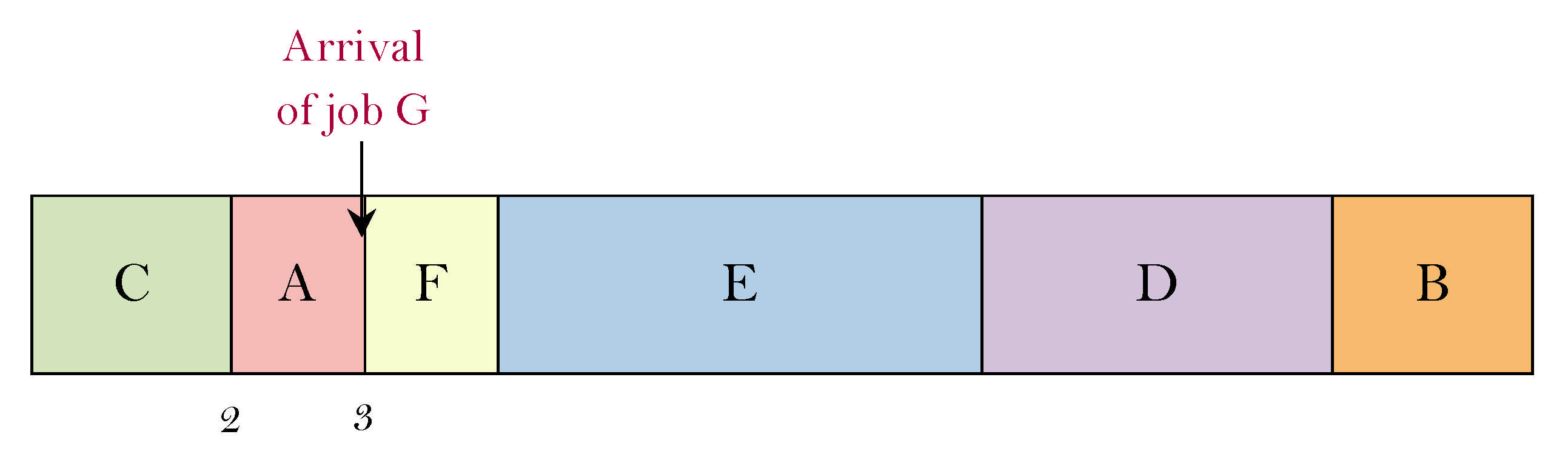
The job G arrives at r_G = 3, with p_G = 1 and w_G = 1. Coefficient α is set to α = 0.5 (see Figure 5).

The optimal solution becomes CAFEDBG and the optimal value is $\alpha {\displaystyle {\sum }_{j=1}^7{w}_j{W}_j}+\left(1-\alpha \right){\displaystyle {\sum }_{j=1}^6{w}_j(C_j-C{o}_j)}=29$. The new optimal solution is given in

Table 5. Optimal solution after disruption caused by job G arrival.

Job	C	A	F	E	D	B	G
pj	2	1	1	4	3	2	1
rj	0	1	2	2	0	1	3
wj	4	5	5	3	2	1	1
Cj	2	3	4	8	11	13	14
wjWj	0	5	5	6	16	10	10
wj(Cj-Coj)	0	0	0	3	2	1

.

6. Numerical Results

The proposed MILP model is programed on the solver FICO Xpress IVE. The simulations have been performed on a Core i7 2.90 GHz laptop. The model implementation has been designed accordingly to the chart presented on Figure 3. In the following section, a detailed explanation of the data generation.

6.1. Instances Generation

The study has been conducted on different instances. It allowed giving, at each rescheduling step, an optimal solution.

Table 6. Parameter values.

Parameters	Values
wj	~U (1, 5)
pjm	~U (1, 4) (ut)
T	48 (ut)

presents the used parameters.

The data that have been chosen can be adapted for real cases, either in a hospital or in an industrial environment. The unit of time (ut) is equivalent to a time duration which may correspond to a real situation. In our case, it is assumed that Δt = 1 ut and 1 ut corresponds to 10 min, i.e., every 10 min, an event may occur (arrival of a new order or arrival of a new urgent patient). Most important in our case, is to define the other problem data (p_j and r_j) with the same unit of time, in order to be closer to a fair situation. The simulation has been conducted over an 8 h time horizon (480 min) representing a hospital or a factory opening time. Hence, T = 8 h = 480 min = 48 ut. The weight values can represent the 5 customers priority or the five emergency levels. The processing times can represent the durations of chirurgical operations or product manufacturing times. It is assumed that it follow a uniform distribution between 1 and 4, obtaining operations of 1 ut (10 min) to 4 ut (40 min). The values of the variable θ(t) are randomly generated using the Bernoulli distribution, giving, at each time t, a value one with probability p_θ and zero with probability 1 − p_θ. By definition, p_θ ϵ [0,1]. It represents the appearance frequency of a job at each step. We start by testing a small appearance frequency, p_θ = 0.2, since under 0.2 there is not enough disruptions. We have tested then with a medium appearance frequency, p_θ = 0.5. Then, we have varied p_θ up to 0.7 until the MILP becomes unable to solve the problem in a reasonable time. Thus, four main studies are established. At first, the impact of the efficiency-stability coefficient α on the schedules. Secondly, the impact of the weight increasing effect on the system. Then, a comparative analysis of the proposed method with other heuristics and dispatching rules. Finally, the computing time of the MILP resolution on different instances for exploring its limitations according to jobs number.

6.2. Impact of the Efficiency-Stability Coefficient α on the Schedules

In this study, the value of α is varied from 0.5 to 1 to study its impact on the optimal schedule. It is assumed that the TWWT is a principal criterion and the TWCTD is a secondary one. Thus, the values of α inferior to 0.5 are not tested. If α becomes too small, the schedule efficiency will be negligible and the situation will be unrealistic in real-life problems. The study has been conducted and analyzed for 10 different instances, generated accordingly to the parameters presented in Section 5.1. We present, in the following example, the results obtained on the instance presented in Table 1.

Example 3.

After resolution of the initialproblem (seeTable 2), it is assumed that new jobs occur disrupting the system. A total of 20 jobs are treated online. The obtained results are given in

Table 7. Influence of α on the optimal schedules.

α	(1)	(2)	(3)	(1)	(2)	(3)	(1)	(2)	(3)	(1)	(2)	(3)
	2nd Schedule			3rd Schedule			4th Schedule			5th Schedule
1	42	11	42	49	17	49	63	29	63	84	47	84
0.9	42	6	38.4	49	12	45.3	63	24	59.1	84	42	79.8
0.8	42	6	34.8	49	12	41.6	63	24	55.2	84	42	75.6
0.7	42	6	31.2	50	9	37.7	66	15	50.7	90	24	70.2
0.6	42	6	27.6	51	7	33.4	69	9	45	96	12	62.4
0.5	42	6	24	52	6	29	69	9	39	99	9	54
	6th Schedule			7th Schedule			8th Schedule			9th Schedule
1	95	49	95	102	56	102	119	64	119	143	76	143
0.9	95	42	89.7	102	49	96.7	119	57	112.8	143	69	135.6
0.8	95	42	84.4	102	49	91.4	119	57	106.6	143	69	128.2
0.7	101	24	77.9	113	31	88.4	127	45	102.4	151	57	122.8
0.6	107	12	69	120	20	80	142	24	94.8	172	30	115.2
0.5	110	9	59.5	123	17	70	139	24	81.5	169	30	99.5
	10th Schedule			11th Schedule			12th Schedule			13th Schedule
1	153	84	153	163	84	163	170	89	170	175	94	175
0.9	153	77	145.4	163	77	154.4	170	82	161.2	175	87	166.2
0.8	153	77	137.8	163	77	145.8	170	82	152.4	175	87	157.4
0.7	161	65	132.2	171	65	139.2	178	70	145.6	183	75	150.6
0.6	188	32	125.6	198	32	131.6	209	35	139.4	218	38	146
0.5	185	32	108.5	195	32	113.5	206	35	120.5	215	38	126.5
	14th Schedule			15th Schedule			16th Schedule			17th Schedule
1	183	94	183	187	98	187	191	101	191	197	107	197
0.9	183	87	173.4	187	91	177.4	191	94	181.3	197	100	187.3
0.8	183	87	163.8	187	91	167.8	191	94	171.6	197	100	177.6
0.7	191	75	156.2	195	79	160.2	199	82	163.9	205	88	169.9
0.6	226	38	150.8	230	42	154.8	234	45	158.4	240	51	164.4
0.5	223	38	130.5	230	39	134.5	237	39	138	249	42	145.5
	18th Schedule			19th Schedule			20th Schedule			21th Schedule
1	206	116	206	210	119	210	216	125	216	226	144	226
0.9	206	109	196.3	210	112	200.2	216	118	206.2	226	128	216.2
0.8	206	109	186.6	210	112	190.4	216	118	196.4	226	128	206.4
0.7	217	88	178.3	221	92	182.3	231	97	190.8	238	125	204.1
0.6	252	51	171.6	256	55	175.6	266	60	183.6	270	94	199.6
0.5	261	42	151.5	268	42	155	284	48	166	288	82	185
(1): TWWT (2): TWCTD (3): The value of the objective function

.

In Table 7, p_θ = 0.5 (20 jobs appeared in a time horizon of 48 ut). At each disruption, the jobs are rescheduled and three values are extracted, the value of TWWT, the value of TWCTD and the value the objective function combining TWWT and TWCTD thanks to α. We have also numbered the schedules with their step numbers.

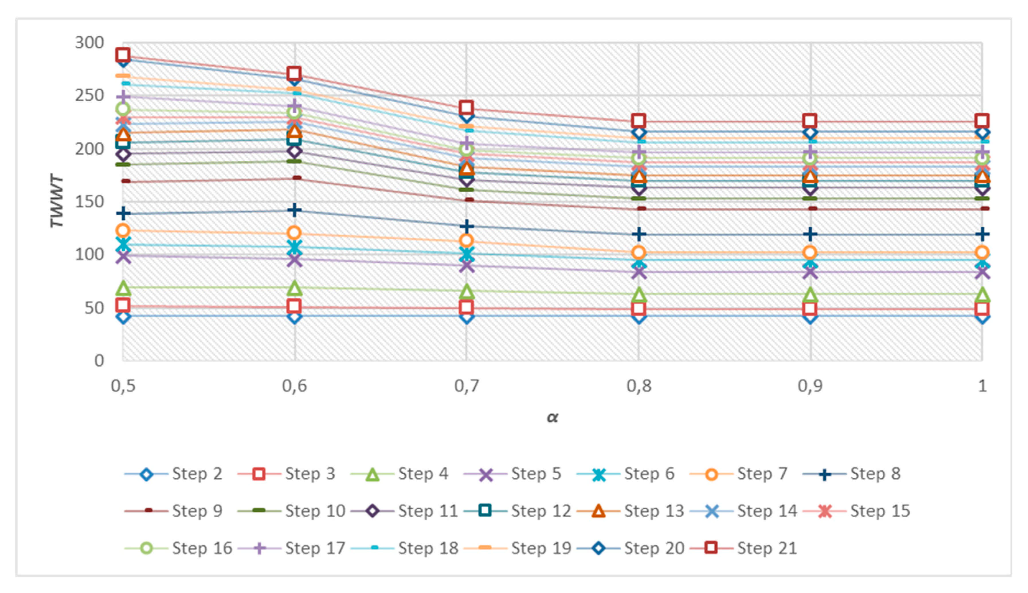
When α = 1, the objective function only considers the efficiency criterion, TWWT. In this case, when the release dates are equal, wSPT-rule is optimal for this problem. Otherwise, the jobs have been scheduled according to its weight and its processing time.

When α decreases, the schedule stability is more considered. Hence, a diminution of a stability criterion TWCTD values is observed, as well as an increase on the values of TWWT. This increase becomes larger in the last steps when the number of jobs is larger (see Figure 6).

The more disruptions, the higher the value of TWWT. In fact, the increase of TWWT in the last steps signifies that there are some jobs that stay for a long time in the system. This increase becomes large when α decreases. To illustrate this phenomenon, we present hereafter the first five jobs disposition in the schedule (see

Table 8. The first five jobs disposition.

α	Initial Schedule	(1)	(2)	2nd Schedule	(1)	(2)	3rd Schedule	(1)	(2)
1	C-A-E-D-B	31	-	C-F-A-E-D-B	42	11	C-F-A-G-E-D-B	49	17
0.9				C-A-F-E-D-B	42	6	C-A-F-G-E-D-B	49	12
0.8				C-A-F-E-D-B	42	6	C-A-F-G-E-D-B	49	12
0.7				C-A-F-E-D-B	42	6	C-A-F-E-G-D-B	50	9
0.6				C-A-F-E-D-B	42	6	C-A-F-E-D-G-B	51	7
0.5				C-A-F-E-D-B	42	6	C-A-F-E-D-B-G	52	6
α	4th schedule	(1)	(2)	5th schedule	(1)	(2)
1	C-F-A-G-H-E-D-B	63	29	C-F-A-G-H-I-E-D-B	84	47
0.9	C-A-F-G-H-E-D-B	63	24	C-A-F-G-H-I-E-D-B	84	42
0.8	C-A-F-G-H-E-D-B	63	24	C-A-F-G-H-I-E-D-B	84	42
0.7	C-A-F-E-G-H-D-B	66	15	C-A-F-E-G-H-I-D-B	90	24
0.6	C-A-F-E-D-G-H-B	69	9	C-A-F-E-D-G-H-I-B	96	12
0.5	C-A-F-E-D-G-H-B	69	9	C-A-F-E-D-G-H-B-I	99	9
(1): TWWT (2): TWCTD

).

The increase of the TWWT at each rescheduling step is due to the low-weight jobs. These jobs move forwards after each disruption, since the new arriving jobs are included in the middle of the sequence, when they have a high weight.

However, when α decreases, the stability criterion is more considered. Thus, the existing jobs make less movement, so as not to disrupt the previous sequence. Therefore, the new arriving jobs are placed lastly which also impacts the value of TWWT in the case they have a high weight. This explains the increase of the TWWT with the small α values.

Remark 1. 

The high weight jobs are always prioritized. Consequently, the jobs with low weights are delayed, even if they arrive early (the case of job B in the example). In fact, the low-weight jobs move forwards at every rescheduling step. There are few chances for these jobs to be executed. To deal with this problem, an innovative concept is conceived. It consists in increasing the jobs weight in function of the time. This is the purpose of Section 5.3.

To analyze the behavior of the criteria with respect to the number of jobs, we studied the variation of the final values of TWWT, TWCD and the objective function for different values of α and p_θ. Ten different instances have been generated, according to the parameters of Section 5.1. Each instance starts by 5 initial jobs. Then, it will be disrupted by the new jobs’ arrival, with an appearance frequency respectively equal to 0.2, 0.5 and 0.6. Averages are presented in

Table 9. Averages of TWWT, TWCTD and objective function, for different values of α and p_θ.

	pθ = 0.2			pθ = 0.5			pθ = 0.6
α	(1)	(2)	(3)	(1)	(2)	(3)	(1)	(2)	(3)
0.5	60.9	9.4	35.15	240.4	61.7	151.05	305.3	79.4	192.35
0.6	59.3	11	39.98	228.2	72.8	166.04	283.6	93.4	207.52
0.7	59.2	12.4	45.16	218.5	91	180.25	277	115.6	228.58
0.8	58.5	14.5	49.7	207.8	106.9	187.62	265.5	137.1	239.82
0.9	58.4	15.3	54.09	206.8	108.2	196.94	265.3	137.9	252.56
1	58.4	16.8	58.4	205.5	119.5	205.5	261.2	154.6	261.2
(1): Average TWWT (2): Average TWCTD (3): Average of the objective function

.

The increase of α helps the TWWT, since its average value decreases with α. However, the average of TWCTD increases with α since the stability has less priority. This behavior is more observed when p_θ increases, i.e., when the number of appearing jobs increases. In the case when the system is more disrupted by the new jobs arrivals, the possibility of having high weight jobs increases, as well as the possibility to delay the low weight jobs. Hence, the increase of their weights in function of time is judicious. Other tests have been performed with p_θ exceeding 0.6, but the MILP fails to solve the problem in a reasonable time.

6.3. The Weight Increasing Effect

As mentioned above, the jobs with low weights are always placed in the last place in the sequence. Thus, it is consistent to proceed with dynamic weights. Thus, the weights become in function of time, release date r_j and the weight index ρ. The proposed formula is given by: $w_{jt}=\hspace{0.17em}{w}_j{(t-r_j+1)}^{\rho }$. ρ allows regulating the weight increasing effect. It is assumed that its value is between 0 and 1 for obtaining relatively small augmentation of the weight values. The case when ρ = 0 signifies that the jobs’ weights are static and no variation of the weight occurs over the time. Otherwise, when ρ = 1, the weight variation becomes too large and may impact the schedule efficiency. Choosing a value of ρ that exceeds 1 becomes unrealistic. Therefore, the selected range for ρ is [0,1]. Thanks to this new formula, the weight becomes in function of the time t. $(t-r_j+1)$ is the difference between the current time and the release date of the job j. If t = r_j, we would obtain a weight equal to zero, which is not the aimed effect. So, we have added plus one. Hence, the new objective function will be:

$$Min\hspace{0.17em}\alpha {\displaystyle \sum _{j=1}^{n\prime }{w}_{jt}{W}_j}+\left(1-\alpha \right){\displaystyle \sum _{j=1}^{n\prime -z}{w}_{jt}(C_j-C{o}_j)}$$

This new weight expression helps the low weight earliest jobs to not wait too long time in the system, through increasing their weights in function of the time. The dates of jobs arrival are defined by their release dates r_j and the dates of their execution by their completion times C_j. Thus, to discuss the trade-off involved while increasing the weight in function of time, we analyzed two criteria. The first one is the Mean Flow Time (MFT), $MFT=\raisebox{1ex}{$1$}\!\left/ \!\raisebox{-1ex}{$n\prime $}\right.{\displaystyle \sum _{j=1}^{n\prime }(C_j-r_j)}$, which measures the sum of the jobs flowtimes divided by n’. The flow time of a job measures the duration between its release date and its completion time, $F_j=C_j-r_j$. The second one is the standard deviation of the flowtime. It assesses the deviations of the jobs’ flowtimes from the MFT.

Table 10. The variation of MFT and standard deviation in function of ρ and α.

	α = 0.5		α = 0.6		α = 0.7		α = 0.8		α = 0.9		α = 1
ρ	MFT	Std Dev	MFT	Std Dev	MFT	Std Dev	MFT	Std Dev	MFT	Std Dev	MFT	Std Dev
0	7.8	6.5	7.8	6.5	7.8	6.5	7.8	6.5	7.8	6.5	7.9	6.59
0.1	7.8	6.5	7.8	6.5	7.8	6.5	7.8	6.5	7.8	6.5	7.8	6.5
0.2	7.8	6.5	7.8	6.5	7.8	6.5	7.8	6.5	7.8	6.5	7.8	6.5
0.3	7.8	6.5	7.8	6.5	7.8	6.5	7.8	6.5	7.8	6.5	7.8	6.5
0.4	7.8	5.87	7.8	5.87	7.8	5.87	7.8	5.87	7.8	5.87	7.8	5.87
0.5	8	5.21	8	5.21	8	5.21	8.1	5.5	8.1	5.5	8.1	5.5
0.6	8	5.21	8	5.21	8	5.21	8	5.21	8.1	5.5	8.1	5.5
0.7	8	5.21	8	5.21	8	5.21	8	5.21	8	5.21	8.1	5.5
0.8	8.2	5.09	8.2	5.09	8.2	5.09	8.2	5.09	8.2	5.09	8.2	5.09
0.9	8.2	5.09	8.2	5.09	8.2	5.09	8.2	5.09	8.2	5.09	8.2	5.09
1	8.2	5.09	8.2	5.09	8.2	5.09	8.2	5.09	8.2	5.09	8.2	5.09
MFT: Mean Flowtime, Std dev: Standard deviation of flowtimes

presents the obtained results for the same instance as the one studied in Section 5.2. The variation of ρ is from 0 to 1 and α from 0.5 to 1.

As can be seen, the increase of ρ increases the value of MFT. However, the standard deviation of the flowtimes decreases. This means that the dispersion around the MFT decreases. In other words, the values of F_j approximate to each other. Thus, the increase of ρ helps the low weight jobs to be scheduled.

On the other hand, the increase of α makes it difficult to decrease the standard deviation of the flowtimes. For example, the standard deviation of the flowtimes with ρ=0.6 is equal to 5.5 when α = 1, instead of 5.21 when α = 0.5. When α decreases, the stability criterion is more considered. Systemically, the new arriving jobs are placed at the end of the schedule, so as not to disrupt the established schedule. As well, the low-weight earliest jobs are systematically executed. Otherwise, if the value of α increases, the efficiency criterion is more considered, the system then will be more disrupted. In this case, a high value of ρ is needed. In conclusion, if α increases, the weight index ρ must also increase, to help the low weight jobs to be scheduled.

To analyze the overheads of the weight index, the variation of the objectives’ values is studied for different values of ρ. Thus, for each value of ρ, the final value of TWWT, TWCTD and the objective function, with w_j, as well as the percentage deviation of the objective function from the static weights case are presented. The study is performed on the same instance, to ensure comparability of results. It is also assumed that α = 0.8. In addition, different values of p_θare experimented. The results are presented in

Table 11. Variation of TWWT, TWCTD and objective function in function of ρ, with different values of p_θ.

	pθ = 0.2				pθ = 0.5				pθ = 0.6
ρ	(1)	(2)	(3)	(4)	(1)	(2)	(3)	(4)	(1)	(2)	(3)	(4)
0	62	8	51.2	0%	226	128	206.4	0%	349	210	321.2	0%
0.1	62	8	51.2	0%	268	104	235.2	14%	377	185	338.6	5%
0.2	62	8	51.2	0%	277	87	239	16%	416	151	363	13%
0.3	62	8	51.2	0%	297	59	249.4	21%	477	110	403.6	26%
0.4	62	8	51.2	0%	362	53	330.2	60%	517	84	430.4	34%
0.5	62	8	51.2	0%	393	43	323	56%	625	72	514.4	60%
0.6	68	6	55.6	9%	443	39	362.2	75%	727	52	592	84%
0.7	68	6	55.6	9%	493	23	399	93%	809	37	654.6	104%
0.8	68	6	55.6	9%	513	17	413.8	100%	848	25	683.4	113%
0.9	68	6	55.6	9%	513	17	413.8	100%	848	25	683.4	113%
1	68	6	55.6	9%	516	16	416	102%	848	25	683.4	113%
(1): TWWT (2): TWCTD (3): The value of the objective function (4): percentage deviation

.

The increase of the weight index ρ helps the system stability since the value of TWCTD decreases. The earliest jobs must keep the same position to be executed. However, the TWWT increases with ρ, since the stability becomes of more priority. An increase in the objective function value is also observed, larger when p_θ = 0.6. In this case, the manager must make a decision about the use of the weight index or not. Other tests have been performed with p_θ exceeding 0.6, but the MILP fails to solve the problem in a reasonable time.

6.4. Comparative Analysis

As mentioned in the introduction section, some papers consider different dispatching rules and heuristics to implement the reactive approach for rescheduling the jobs in response to disruptions. Some frequently used dispatching rules and heuristics are mentioned in [80]. Among them, we select FIFO (first in first out) to compare with the proposed MILP, since it is commonly used in industrial companies, when not any rescheduling strategy is implemented [43]. In addition, it is also interesting to compare with some heuristic considering the jobs’ weights. In [81], the authors compared their proposed heuristics based on MILP with wSPT, since they also considered the jobs’ weights in a flowshop rescheduling problem. Therefore, we adapted these two heuristics, FIFO and wSPT, to match our problem. Ten different instances are tested. Each instance starts with 5 initial jobs, then it will be disrupted, at each step, by the arrival of a new job with the appearance frequency p_θ respectively equal to 0.2, 0.6 and 0.7. Averages are presented in

Table 12. Comparison of the results for different solving methods.

		MILP				wSPT				FIFO
pθ (TNAJ)	α	(1)	(2)	(3)	(4)	(1)	(2)	(3)	(4)	(1)	(2)	(3)	(4)
0.2 (10 jobs)	0.5	60.9	9.4	35.15	0.59	67.4	22.7	48.1	0.08	104.8	0	52.4	0.06
	0.75	59.2	12.4	47.5	0.62	67.4	22.7	56.225	0.08	104.8	0	78.6	0.06
	1	58.4	16.8	58.4	0.76	67.4	22.7	61.9078	0.08	104.8	0	104.8	0.06
0.6 (28 jobs)	0.5	305.3	79.4	192.35	247.8	286.7	162.9	224.8	0.08	596	0	298	0.07
	0.75	277.3	121.7	238.5	242.1	286.7	162.9	255.75	0.09	596	0	447	0.08
	1	261.3	154.6	261.2	235.6	286.7	162.9	286.7	0.1	596	0	596	0.08
0.7 (33 jobs)	0.5	770.42	212	491.21	1746.98	758	479.2	618.6	0.28	1523.8	0	761.9	0.11
	0.75	665.28	379.71	593.89	9530.24	758	479.2	688.3	0.28	1523.8	0	1110.6	0.12
	1	646.42	445.85	646.42	1606.10	758	479.2	758	0.29	1523.8	0	1523.8	0.10
(1): TWWT (2): TWCTD (3): Objective function (4): Computing time (in seconds) TNAJ: Total Number of Appearing jobs

.

The proposed MILP always provides better solution than wSPT and FIFO. wSPT which consists in sequencing the jobs by increasing order of p_i/w_i misses some optimal solutions since, in the presence of the release dates, this heuristic becomes not able to optimally solve the problem. In addition, it does not take into account the stability aspect. However, FIFO which consists in placing, at each rescheduling step, the new job in the last position, provides bad solutions. Even if FIFO heuristic gives stable sequences, it is weak in terms of efficiency since it does not consider the weights to construct the schedules. Indeed, when α increases, the schedule efficiency becomes more important. In this case, FIFO solution moves away from MILP solution, this gap becomes wider when the number of jobs is important. Figure 7 depicts this behavior.

In terms of computation time, the two heuristics, wSPT and FIFO, are very fast compared to the MILP method. Using this latter heuristic, a break is observed when p_θ = 0.7. In the following, a thorough study of the computing time is presented.

6.5. Computing Time Study

To analyse the maximum time spent in an iteration, in this study, we tested the maximum duration of an iteration (MDI) for the model resolution on different instances. The study has been performed on the solver FICO Xpress IVE, on a laptop of a Core i7 2.90 GHz. Ten different instances per problem size are tested. These are generated randomly, using the values of Section 5.1. Then, the maximums, the minimums, the averages and the standard deviations of MDI in seconds are calculated. We have tested sets of instances containing respectively 5 and 7 initial jobs. Then, over a horizon of T = 48 ut, we have disrupted these jobs by the arrival of new ones. α is given by 0.8. Different values of p_θ are tested (0.2; 0.5; 0.6; 0.7) to analyze its impact on the MDI. The obtained results are given in

Table 13. Maximum duration of an iteration (MDI).

Initial Jobs	pθ (TNAJ)	Min MDI (s)	Max MDI (s)	Avg MDI (s)	Std Dev MDI (s)
5	0.2 (10 jobs)	0.06	0.08	0.07	0.009
	0.5 (24 jobs)	0.38	0.42	0.4	0.01
	0.6 (28 jobs)	12.87	562.72	232.78	234.02
	0.7 (33 jobs)	56.34	3562.34	1107.67	1666.78
7	0.2 (10 jobs)	0.09	0.11	0.10	0.006
	0.5 (24 jobs)	0.56	0.82	0.63	0.10
	0.6 (28 jobs)	35.49	593.09	306.20	261.02
	0.7 (33 jobs)	-	-	-	-
TNAJ: Total Number of Appearing Jobs

.

The set of jobs that must be executed, at each iteration, increases too much with p_θ, as well as the average of the MDI. This later increases also with the set of initial jobs. Thus, the average of MDI depends on both, the appearance frequency of the jobs and the set of initial jobs. If these ones become large, the average and the standard deviation of the MDI increase. This matter makes it difficult to estimate the necessary computing time that the MILP needs for solving the problem.

In the dynamic environments, the decision makers must establish a planning after each disruption. This one should be constructed as soon as possible, in preference before the occurrence of another disruption. In our case, according to the discretization that we have assumed, the arrival of a new job can be possible at each Δt. So, if the MDI exceeds Δt, it is considered as an unacceptable time. Based on the assumption assuming that Δt is equivalent to 10 min (600 s) and according to Table 13, the proposed MILP model is effective in solving the problems made up of 7 initial jobs subjected to disruptions which occur at each period with an appearance frequency up to 0.6. It is averagely equivalent to 35 jobs in total. We have also performed the problems for 7 initial jobs with p_θ = 0.7 (40 jobs). The program ran for 12 h. Then, we have interrupted the simulation.

7. Conclusions and Perspectives

In this paper, a new optimization criterion is proposed to evaluate the performance of the schedules on a single machine rescheduling problem. This new criterion combines simultaneously the total weighted waiting time as a schedule efficiency and the total weighted completion time deviation as a schedule stability. This association of criteria has never been studied in the literature before and it can be a very helpful and significant criterion in industrial and hospital environments. A MILP model is proposed and an iterative predictive reactive strategy is established for dealing with the online part. In dynamic environments, the rescheduling is often used to organize the production activities. In such situations, the customer priority has a major importance, since it defines which order to prioritize. Therefore, it was consistent to consider this factor on the performance measure. Thus, the weights are considered in the efficiency and stability criterion. However, by testing our approach, we have observed that the low weighted operations may be constantly postponed by the occurrence of new high weighted operations, the solution proposed to overcome this drawback consists in varying the weight of operations in function of the time spent in the system. In this case, the challenge will be how to regulate the weight variation so as not to impact the schedule efficiency. The established study demonstrates a large percentage deviation of the objective function from the case of the static weights, but the proposed conception helps the low weighted operations to be executed. The model resolution allows us to conclude that:

-

The increase of the TWWT at each rescheduling step is due to the low-weight jobs. These jobs move forwards after each disruption since the new arriving jobs are included in the middle of the schedule.

-

Increasing the weight in function of the time helps the low weight earliest jobs to be executed. However, the values of the weight index must be increased for the high values of α.

-

Analyzing the maximum duration of iteration, the computing time depends on both the set of initial jobs and the appearance frequency of the jobs.

This work can be of great interest for the decision makers that manage rescheduling systems in hospital or industrial environments. It can help them to provide, at each rescheduling step, an optimal schedule for a single machine problem. The main limitation of this work is the number of the jobs. Firstly, we have considered only one job arrives per period. Secondly, the MILP is limited to averagely solve 35 jobs in a horizon of 48 ut (equivalent to 8 h). At those time, even before COVID-19 disaster, the pressure on healthcare services is continuously increasing. In fact, the hospital decision makers must quickly establish a planning in response to the emergency patients’ arrival, even if several ones arrive at the same time. Thus, the execution time is also an interesting debate. Heuristics wSPT and FIFO have proved their speed to cope with this kind of problem, but their efficiency is weak compared the MILP resolution. Therefore, one of the main short-term prospects is to design efficient heuristics and metaheuristics to browse even more jobs in a reasonable time, as well as a comparison of the proposed approximate methods with other existing heuristics. We will also consider multi machines problems at middle-term research objective.