Fibers Effects on Contract Turbulence Using a Coupling Euler Model

Abstract

Fiber additive will induce the rheological behavior of suspension, resulting in variation in velocity profile and fiber orientation especially for the non-dilute case. Based on the fluid-solid coupling dynamics simulation, it shows that the fiber orientation aligns along the streamline more and more quickly in the central turbulent region as the fiber concentration increases, especially contract ratio Cx > 4. However, fibers tend to maintain the original uniform orientation and are rarely affected by the contract ratio in the boundary layer. The fibers orientation in the near semi-dilute phase is lower than that in the dilute phase near the outlet, which may be the result of the hydrodynamic contact lubrication between fibers. The orientation distribution and concentration of the fibers change the viscous flow mechanism of the suspension microscopically, which makes a velocity profile vary with the phase concentration. The velocity profile of the approaching semi-dilute phase sublayer is higher than that of the dilute and semi-dilute phases on the central streamline and in the viscous bottom layer, showing weak drag reduction while the situation is opposite on the logarithmic layer of the boundary layer. The relevant research can provide a process strategy for fiber orientation optimization and rheological control in the industrial applications of suspension.

1. Introduction

Fiber suspensions are widely used in many fields, such as wood pulp used in the modern papermaking industry. Main components of the mixture are water and the fibers. Previous studies have indicated that the addition of fibers can change the transport properties of the flow field, and in turn influence the fibers orientation and distribution, which will ultimately affect the quality of finished products. Related studies focus on the pipe and channel flow more than the contraction.

Contract flow is mainly used to accelerate the flow rate, such as jet nozzle and the headbox. The headbox is the key part of the modern paper machine, which can produce high intensity micro-turbulence to effectively disperse the fibers and determine their distribution along the horizontal and longitudinal direction of paper. Thus, it can prevent the fiber from settling and flocculating to improve the strength of the paper sheet. The internal flow field in the headbox is similar to the turbulent contraction. The contraction ratio C_x is an important parameter of the contract field, which is the ratio of the local average velocity to the inlet average velocity. In view of the complexity of the fluid-solid coupling mechanism between the carrier fluid and the fibers, some simulations have been made in many researches. Harris et al. [1], Ullmar et al. [2,3] and Zhang [4] studied the fiber orientation distribution in the dilute turbulent contraction. It is found that the anisotropy of fibers orientation is mainly determined by the contraction ratio rather than the Reynolds number. Increasing contraction ratio would increase fiber alignment significantly and vice versa. Because the turbulent effect is not taken into account in their studies, the relationship between the orientation anisotropy of the fibers and the turbulence pulsation of the flow field is not known clearly.

Olson et al. [5] thought that fibers orientation depends on the combined effect of fibers motion and turbulence. Ignoring the influence of the latter is the reason why the theoretical prediction of fiber orientation alignment is higher than the experimental measurements. Then Olson et al. [6] used the Euler model to predict the fiber orientation distribution. When the contraction ratio grew from 5 to 50, the fiber alignment increases obviously. The fibers orientation distribution changed slightly with inlet velocity. Parsheh et al. [7,8] analyzed the effects of four kinds of wall shapes on the anisotropy of fiber orientation by ignoring the interaction between fibers and fluids. It was shown that the anisotropy of fibers orientation varied with the contract shape and was dominated by the rotating Peclet number. When the contract ratio and Peclet number are both large, the turbulence effect can be ignored. Otherwise, turbulence has a great influence on fiber orientation. Lin et al. [9] used slender body theory to simulate fiber orientation distribution. Then Lin et al. [10] obtained the orientation angle of a single fiber by the analytical and numerical method and concluded that contraction ratio had an important effect on fiber orientation distribution. Yang [11] gave the optimal contract wall for desired fibers orientation in dilute suspension by the one-way coupling RSM method.

The existing methods mainly consider the effect of the carrier fluid on the fibers (e.g., Olson [5,6,12], Gillissen [13] and Johnson etc. [14]). In fact, the effect of additive on the turbulence varies with its concentration and scale (e.g., Lin etc. [10,15,16,17] and Yang etc. [18]). Therefore, the coupling numerical simulation will contribute to a further research about the orientation characteristics of the fiber under the different additive concentration. It’ll also achieve a better control over flow behaviors during the fiber-reinforced materials production.

2. Coupling Models and Methods

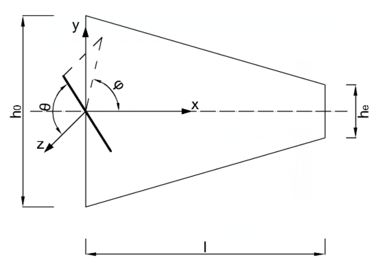
In order to understand the interaction mechanism between the fluid-solid phases of fibers suspension, the variation of fiber orientation and flow velocity profile with the additive concentration nL³ and the contract ratio Cx is mainly studied in the contract turbulence.

2.1. Models

Based on Parsheh’s experiment [7] the two-dimensional model of axisymmetric contraction is shown in Figure 1. The coordinate origin is located at the inlet of the flow field. The contraction length l is 550 mm, inlet height h₀ is 179.2 mm, outlet height h_e is 16 mm and the maximum contraction ratio C_max is about 11.2. The angle between the projection of the fiber orientation P on the x-y plane and the X-axis is ϕ. The angle between fiber orientation P and Z-axis is θ. X-axis is along the flow direction; Y-axis is vertical to the flow direction and Z-axis is the span direction of the flow.

2.2. Mathematical Description of Fibers Orientation Distribution

There are two premises to assure that the suspension flow can be regarded as a single continuum medium: (1) The size of the added particles would be much smaller than the characteristic scale of the flow field and the suspension is quasi-uniform; (2) The Reynolds number of the particles, characterized by the relative velocity of the particles in the flow field, should be small enough to satisfy the quasi-Newtonian fluid.

Therefore, the flow behavior of the fiber suspension can be described by using Euler method. The orientation state of abundant suspended fibers in the dilute flow is described by a Fokker-Plank type function $f(t,x,\varphi )$, which is the probability of a fiber orienting p occurring at time t and placement x. Considering the turbulent effect according to the Reynolds average idea, Equation (1) is given for a 2D steady incompressible flow and its detailed derivation is shown in the literature [18].

$$\frac{{\partial }^2\overline{f}}{{\partial }^2\varphi }=H\frac{\partial \overline{f}}{\partial \varphi }+R\overline{f}+B\frac{\partial \overline{f}}{\partial x}+G\frac{\partial \overline{f}}{\partial y}$$

(1)

where the coefficients in the Equation (1) can see Equations (2)~(5):

$$B=\frac{{\sin }^2(2\varphi )}{4D_r}\overline{u},$$

(2)

$$G=\frac{{\sin }^2(2\varphi )}{4D_r}\overline{v}$$

(3)

$$H=-\frac{{\sin }^2(2\varphi )}{2D_r}\left(\frac{\partial \overline{u}}{\partial x}\sin (2\varphi )+\frac{\partial \overline{v}}{\partial x}{\sin }^2\varphi -\frac{\partial \overline{u}}{\partial y}{\cos }^2\varphi \right)$$

(4)

$$R=-\frac{{\sin }^2(2\varphi )}{4D_r}\left(\frac{\partial \overline{u}}{\partial x}\cos (2\varphi )+\frac{1}{2}(\frac{\partial \overline{u}}{\partial y}+\frac{\partial \overline{v}}{\partial x})\sin (2\varphi )\right)$$

(5)

Here p is a fiber’s unit orientation vector along the coordinate axes (see Figure 1), i.e., $p={\left(\cos \varphi ,\sin \varphi \right)}^T$. ϕ is an orientation angle of fibers; $D_r={\left[a{\left(\upsilon /\epsilon \right)}^{1/2}+bL{\left(\upsilon \epsilon \right)}^{-1/4}\right]}^{-1}$, is the rotational diffusion rate of fibers; $\upsilon$ is the kinematic viscosity; $\epsilon$ is the turbulent dissipation rate. u, v are the x-component and y-component of flow velocity V respectively.

2.3. Numerical Solution

Equation (1) is similar to the conventional convection-diffusion equation with the convection terms just for the position space and the diffusion terms for the orientation angle space. A difference scheme is adopted like $f_k^{i,j}=f(x_{ij},{\varphi }_k)$.

For the convenience of numerical calculation, the variables in the calculation region, such as 0 ≤ x ≤ M, 0 ≤ y ≤ N, −π/2 ≤ ϕ ≤ π/2, are firstly discretized, like x₀ = 0, x_{i =} x_i−1 + Δx_i, i = 1, 2, …, I, I + 1; y₀ = 0, y_j = y_j−1 + Δy_j, j = 1, 2, …, J, J + 1; ϕ₀ = −π/2, ϕ_k = kΔϕ, k = 1, 2, …, K, K + 1. If a discrete method with high order accuracy is used for the derivative of orientation angle ϕ, it’ll introduce too many angle quantities and make the solution harder. Hence the semi-discrete approximation form is adopted for Equation (1) here and the original partial differential equation can be transformed into an ordinary differential equation with respect to ϕ. Moreover, the fourth-order Runge-Kutta method is suitable for ordinary differential equations, which can improve the accuracy of orientation derivative approximation.

To do this, set $F=\partial \overline{f}/\partial \varphi$ and the original equation can be written as:

$$f^{\prime }=F,f(x_i,y_j,{\varphi }_0)=1/\pi$$

(6)

$$F^{\prime }=Z(x,y,\varphi ,f,F)=R_k^{i,j}{f}_k^{i,j}+H_k^{i,j}{F}_k^{i,j}+B_{{}_k}^{i,j}\frac{{\overline{f}}_{k-1/2}^{i,j}-{\overline{f}}_{k-1/2}^{i-1,j}}{\Delta x_i}+G_k^{i,j}\frac{{\overline{f}}_{k-1/2}^{i,j}-{\overline{f}}_{k-1/2}^{i,j-1}}{\Delta y_j}$$

(7)

Based on the fourth-order Runge-Kutta format, we have:

$$f_{k+1}^{x,y}=f_k^{x,y}+\frac{\Delta \varphi }{6}(K_1+2K_2+2K_3+K_4)$$

(8)

$$F_{k+1}^{x,y}=F_k^{x,y}+\frac{\Delta \varphi }{6}(L_1+2L_2+2L_3+L_4)$$

(9)

where

$$K_1=F_k^{i,j},\begin{array}{ccc}& & \end{array}{L}_1=Z(x_i,y_j,f_k^{i,j},F_k^{i,j})$$

(10)

$$K_2=F_k^{i,j}+\frac{\Delta \varphi }{2}{L}_1\begin{array}{ccc}& & \end{array}{L}_2=Z(x_{i+1/2},y_{j+1/2},f_k^{i,j}+\frac{\Delta \varphi }{2}{K}_1,F_k^{i,j}+\frac{\Delta \varphi }{2}{L}_1)$$

(11)

$$K_3=F_k^{i,j}+\frac{\Delta \varphi }{2}{L}_2\begin{array}{ccc}& & \end{array}{L}_3=Z(x_{i+1/2},y_{j+1/2},f_k^{i,j}+\frac{\Delta \varphi }{2}{K}_2,F_k^{i,j}+\frac{\Delta \varphi }{2}{L}_2)$$

(12)

$$K_4=F_k^{i,j}+\Delta \varphi L_3\begin{array}{ccc}& & \end{array}{L}_4=Z(x_{i+1},y_{j+1},f_k^{i,j}+\Delta \varphi K_3,F_k^{i,j}+\Delta \varphi L_3)$$

(13)

The solution of equations f satisfies the condition ${\displaystyle \oint f}\left(x,p\right)dp=1$ and the periodic condition $\overline{f}\left(\varphi \right)=\overline{f}\left(\varphi +\pi \right)$.

2.4. Coupling Equations of Fiber Suspension Flow

According to the volume concentration nL³ or volume fraction Φ_c of the additive, the suspension flow may be divided into a dilute phase, a semi-dilute phase and a dense phase. It is generally believed that the distance D between fibers is much larger than the fiber length L to meet the condition of nL³ << 1 or Φ_c << a_r⁻² and there is almost no contact between the fibers in the dilute phase. In a semi-dilute phase, the distance D between the fibers is less than L but is much larger than fiber diameter d, that is, D ≤ L & D >> d. Although there are little physical contacts among fibers to meet nL³ >> 1 and nL²d < 1 or a_r⁻² << Φ_c << a_r⁻¹, the fibers are mainly affected by the hydraulic action within a range of fiber length. In the case of a dense phase, the distance D between fibers is a multiple of the fiber diameter d to meet nL²d > 1 or Φ_c >> a_r⁻¹. Here a_{r =} L/d, is the aspect ratio of fibers. n is the number density of fibers.

A coupling Reynolds stress model is needed to reflect the interaction mechanism between the fluid-solid phase of dilute as Equation (14) [19]. Thus compared with Newtonian fluid, the Reynolds average series equation for the suspension will produce the fiber additional stress terms. The concrete forms of the terms are given in detail by Yang etc. [18] and can be found in the Equations (15)–(25). Then the effects of fiber concentration on the carrier fluid were investigated by solving these equations.

$${\tau }_f={\mu }_f(<pppp>-\frac{I}{3}<pp>):E$$

(14)

$$\frac{\partial {\overline{V}}_i}{\partial t}+{\overline{V}}_j\frac{\partial {\overline{V}}_i}{\partial x_j}=(\cdots )+Q_i^V$$

(15)

$$Q_i^V=\frac{{\mu }_f}{\rho }\frac{\partial }{\partial x_j}\left((\overline{a_{ijmn}}-\frac{I_{ij}}{3}\overline{a_{mn}})\frac{\partial {\overline{V}}_m}{\partial x_n}\right)$$

(16)

$$\frac{D\overline{({V^{\prime }}_i{V^{\prime }}_j)}}{Dt}=(\cdots )+Q_{ij}^R+S_{ij}^R$$

(17)

$$Q_{ij}^R=\frac{{\mu }_f}{2\mu }\{\frac{\partial }{\partial x_k}\left((\overline{a_{jkmn}}-\frac{I_{jk}}{3}\overline{a_{mn}})\upsilon \frac{\partial \overline{{V^{\prime }}_i{V^{\prime }}_m}}{\partial x_n}\right)+\frac{\partial }{\partial x_k}\left((\overline{a_{ikmn}}-\frac{I_{ik}}{3}\overline{a_{mn}})\upsilon \frac{\partial \overline{{V^{\prime }}_j{V^{\prime }}_m}}{\partial x_n}\right)\}$$

(18)

$$S_{ij}^R=-\frac{{\mu }_f}{\mu }\left({\displaystyle \sum _k(\overline{a_{ikmn}}-\frac{I_{ik}}{3}\overline{a_{mn}})}\frac{2\epsilon }{3}{\delta }_{im}{\delta }_{nk}{\delta }_{ij}\right)$$

(19)

$$\frac{\partial k}{\partial t}+{\overline{V}}_k\frac{\partial k}{\partial x_k}=(\cdots )+Q^k+S^k$$

(20)

$$Q^k=\frac{{\mu }_f}{2\mu }\frac{\partial }{\partial x_k}\left((\overline{a_{ikmn}}-\frac{I_{ik}}{3}\overline{a_{mn}})\upsilon \frac{\partial \overline{{V^{\prime }}_i{V^{\prime }}_m}}{\partial x_n}\right)$$

(21)

$$S^k=-\frac{{\mu }_f}{\mu }\left({\displaystyle \sum _{i,k}(\overline{a_{ikmn}}-\frac{I_{ik}}{3}\overline{a_{mn}})}\frac{\epsilon }{3}{\delta }_{im}{\delta }_{nk}\right)$$

(22)

$$\frac{D\epsilon }{Dt}=(\cdots )+\frac{{\mu }_f}{\mu }\left(Q^S+S^S\right)$$

(23)

$$\begin{array}{l}{Q}^S=2\upsilon \frac{{\partial }^2}{\partial x_j\partial x_k}\left({\displaystyle \sum _{i,n}(\overline{a_{ijmn}}-\frac{I_{ij}}{3}\overline{a_{mn}})\frac{\epsilon }{3}{\delta }_{im}{\delta }_{nk}}\right)-\upsilon \frac{\partial }{\partial x_j}\left({\displaystyle \sum _{i,n}(\overline{a_{ijmn}}-\frac{I_{ij}}{3}\overline{a_{mn}})\frac{\partial }{\partial x_k}(\frac{\epsilon }{3}){\delta }_{im}{\delta }_{nk}}\right)\\ -\upsilon {\displaystyle \sum _{i,n}\frac{\partial (\overline{a_{ijmn}}-\frac{I_{ij}}{3}\overline{a_{mn}})}{\partial x_k}}\frac{\partial }{\partial x_k}(\frac{\epsilon }{3}){\delta }_{im}{\delta }_{nj}\end{array}$$

(24)

$$S^S=-{\displaystyle \sum _{i,n}(\overline{a_{ijmn}}-\frac{I_{ij}}{3}\overline{a_{mn}})\frac{{\epsilon }^2}{3k}}{C}_{2\epsilon }\rho {\delta }_{im}{\delta }_{nj}$$

(25)

where: <pppp> and <pp> are the fourth order and second order tensor of averaged fibers orientation respectively $\langle pp\rangle ={\displaystyle \int ppf\left(p,t\right)}dp$, $\langle pppp\rangle ={\displaystyle \int ppppf\left(p,t\right)}dp$; a_ijmn and a_ij are the compents of <pppp> and <pp> respectively. ρ is the density of carrier fluid; τ_f is the fibers additional stress; Here μ is the dynamic viscosity, $\upsilon$ = μ/ρ; μ_f is the additive dynamic viscosity coefficient, ${\mu }_f=\pi n{L}^3\mu \zeta g\left(\xi \right)/6$; $\xi ={[\ln (2a_r)]}^{-1}$;$g(\xi )=\left(1+0.64\xi \right)/\left(1-1.5\xi \right)+1.659{\xi }^2$. E is the strain rate of carrier fluid; V_i is the velocity component of flow field; I_ij is the compent of identity matrix I; $\overline{A}$ is a mean part of the physical quantity A; $A^{\prime }$ is a fluctuating part of A; $(\cdots )$ denotes the terms of original Reynolds equation; k is the turbulent kinetic energy; $\epsilon$ is the turbulent dissipation rate; $C_{2\epsilon }=1.92$.

2.5. Main Numerical Step for Coupling Simulation

The fluid-solid coupling Euler model with fiber additional stress terms can achieve the numerical solutions of the whole computational domain by using the turbulence solver of Fluent. The main calculation steps are as follows:

(1)

Equations (15), (17), (20) and (23)with $Q_i^V=Q_{ij}^R=S_{ij}^R=Q^k=S^k=Q^S=S^S=0$, are solved to get ${\overline{V}}_i$, $\overline{{V^{\prime }}_i{V^{\prime }}_j}$, k and ε of Newtonian fluid.

(2)

Equation (1) is solved by Equations (6)~(13) to get f(x,φ).

(3)

Substitute f(x,φ) into $a_{ijmn}={\displaystyle \int p_i{p}_j}{p}_m{p}_{n}f(x,\phi )d\phi$, $a_{ij}={\displaystyle \int p_i{p}_j}f(x,\phi )d\phi$ to get a_ijmn and a_ij.

(4)

Calculate μ_f with the fiber geometry and concentration parameters.

(5)

Substitute μ_f, a_ijmn, a_ij, ${\overline{V}}_i$, $\overline{{V^{\prime }}_i{V^{\prime }}_j}$, k ε etc. to Equations (15), (17), (20) and (23) with Equations (16), (18), (19), (21), (22), (24) and (25) and update ${\overline{V}}_i$, $\overline{{V^{\prime }}_i{V^{\prime }}_j}$, k and ε of suspension flow after iterative calculation.

(6)

Iteration ends if convergence, otherwise return to step (2) through (5).

3. Validation

The fibers has a nominal length of 3.2 mm, a diameter of 57 um and a volume concentration nL³ of 0.0053 here by Parsheh’s experimental data [7], which is a dilute suspension. It is assumed that the initial condition of fiber distribution is uniform. a₁₁₁₁ is the component of the fourth order tensor <pppp> of averaged fibers orientation and it is an index of fiber orientation alignment. The data of the mean flow field is calculated from the Reynolds Stress Model (RSM) on the inlet conditions as

Table 1. Parameters of carrier fluid.

ε0 (m2/s3)	k0 (m2/s2)	u0 (m/s)	a	b
3.05 × 10−3	1.034 × 10−3	0.4375	8.0	1.2

, and the parameter subscript “0” represents the inlet conditions.

Under the same flow conditions, the one-way coupling and the two-way coupling model are used respectively and then simulation results of mean velocity in the x direction and the orientation distribution a₁₁₁₁ are compared with those of Parsheh et al. [8] in Figure 2.

The simulation results are almost consistent with Parsheh’s. The mean flow is approximately one-dimensional potential one at the central area of the contraction in Figure 2a. When C_x is 2.8, the relative velocity profile is in good agreement with the experimental measured value. When the contraction ratio is 9.0, the simulated data is slightly higher than the experimental value. That’s because the velocity calculation is more easily affected by the grid difference precision when the contraction ratio C_x is large. The overall error between them is no more than 5%, which meets the calculation accuracy.

As shown in Figure 2a,b, the fiber orientation tends to be consistent rapidly with the increase of contraction ratio C, especially above C_x > 2. When C_x < 2, fibers present a local random distribution. This is mainly because the suspended fibers are orientated by turbulent effect and tensile effect in the contraction flow. When the effect of the former is higher than or equal to that of the latter in the flow field, the fiber orientation distribution will be more uniform. On the contrary it will show obvious alignment.

At the same time, simulation shows that there is no significant difference in fiber orientation distribution between one-way coupling and two-way coupling calculation, which indicates that the influence of additional fiber stress term can be ignored for extremely dilute fiber suspended flow, and the unidirectional coupling method can satisfy the calculation accuracy.

4. Results and Discussion

As is known above, the orientation distribution of suspended fibers is easily affected by the local flow in the field with a large contact ratio. The concentration of fibers would affect the distributions of fibers orientation as illustrated in the figures below.

4.1. Effect of Fibers Concentrations on Fibers Orientation

The orientation alignment index $a_{1111}$ is simulated for the suspension of Table 1 by using the coupling RSM model. Six groups of volume concentration parameters including dilute phase ($n{L}^3<<1$) and semi dilute phase ($n{L}^3>>1$ and $n{L}^{2}d<1$) were used. The impact of fibers concentration on fibers orientation is illustrated as Figure 3 and Figure 4 below.

It is showed from the Figure 3 that the fiber orientation aligns along the streamline more and more quickly with the increasing fiber concentration though almost all of the fibers at different concentration have a higher aligning orientation at the outlet. One of the more interesting findings is that the fibers orientations of nL³ = 0.3 and nL³ = 1.2 are not only slightly lower than that of the semi dilute phase nL³ = 4.8 and nL³ = 12 but also slightly lower than that of the dilute phase nL³ = 0.0053 and nL³ = 0.075 near the center streamline. However, the fibers orientations are all close to the even distribution near the wall in Figure 3. It may be inferred that whether the orientation of the suspended fibers is uniform or aligned depends largely on the local flow structure. Moreover, the probability distribution of fiber orientation in a dilute phase is more dependent on the velocity gradient structure of the flow field than that in a semi-dilute phase. With the increase of the contraction ratio, its distribution in the semi-dilute phase shows a certain degree of viscous hysteresis, whose pattern is obviously different from that of velocity field.

From Figure 4, there is little difference between the probability density distribution f(φ) of the orientation angle φ = 0°and φ = 90°near the inlet no matter the fibers concentration. However, with the increase of contract ratio, the higher the concentration is, the more obviously φ = 0°is dominant. At the same time, the probability f(φ) of fibers orientation φ = 60° and φ = 90° decreases sharply in the semi dilute phase, which indicates that the fibers tend to be oriented along the flow direction due to the tensile effect of local flow in the field with large contract ratio.

Based on the near wall velocity, the boundary layer thickness of the case is estimated to be about 1.38 mm. Then the boundary layer grid is divided accordingly. The rest area is a turbulence central region. In the turbulent boundary layer, the fiber orientation alignment index a₁₁₁₁ is shown in the Figure 5.

It is generally believed that the viscous bottom layer is located at the wall distance $0<y^{+}<40$; The corresponding region $y^{+}<5$ is the linear bottom layer, where its velocity presents a linear distribution along the normal direction of the wall. It can be seen from the Figure 5 that the semi-dilute phase is the dividing line. When nL³ > 1, it is more difficult for the fibers to align with the increase of phase concentration in $y^{+}<5$. However, when nL³ < 1 fibers will approach the homogeneous orientation of 1/π more easily with the decrease of phase concentration.

When $40<y^{+}<300$, the flow is in the logarithmic layer where its velocity presents a logarithmic distribution along the normal direction of the wall. The average viscous shear stress in the layer is very small, so the flow is almost controlled by the turbulent shear stress. When the contraction ratio C_x < 2, the turbulent effect is greater than the tensile effect in the boundary layer, and a₁₁₁₁ behaves in a trend of increasing at first and then decreasing along the boundary layer thickness. However, when C_x > 2, a₁₁₁₁ shows a slight upward trend and remains in the range of 0.32~0.40 on the whole, which was close to the uniform orientation.

It can be explained that the viscous damping reduces tangential velocity pulsation and the wall also prevents normal velocity pulsation at the viscous bottom of turbulent boundary so that fibers in this layer are easy to maintain their original orientation. Accordingly, in the influence of the boundary layer the fiber orientation tends to be uniform. Therefore the orientation of fibers near the wall is not easily aligned.

Different from in the turbulent boundary layer, fiber orientation alignment generally increases gradually in the turbulent central region along the direction from the wall to the central streamline, especially when C_x > 4, as shown in Figure 6. When C_x < 4, the evolution curves of a₁₁₁₁ under different phase concentrations is compared. It can be found, obviously, that the higher the phase concentration is, the easier the fibers are to align. The alignment orientation of fiber has the regular characteristics of the fluid viscous interaction and local turbulence structure. At C_x > 4, when the tensile effect of the contracting precedes its turbulent effect gradually, a₁₁₁₁ increases quantitatively with the increasing of C_x. However, the fibers under the semi-dilute concentration nL³ = 0.3 and nL³ = 1.2 have a lower alignment than those of the dilute phase nL³ = 0.0053 and the semi-dilute phase nL³ = 4.8 and nL³ = 12 when C_x = 9.0.

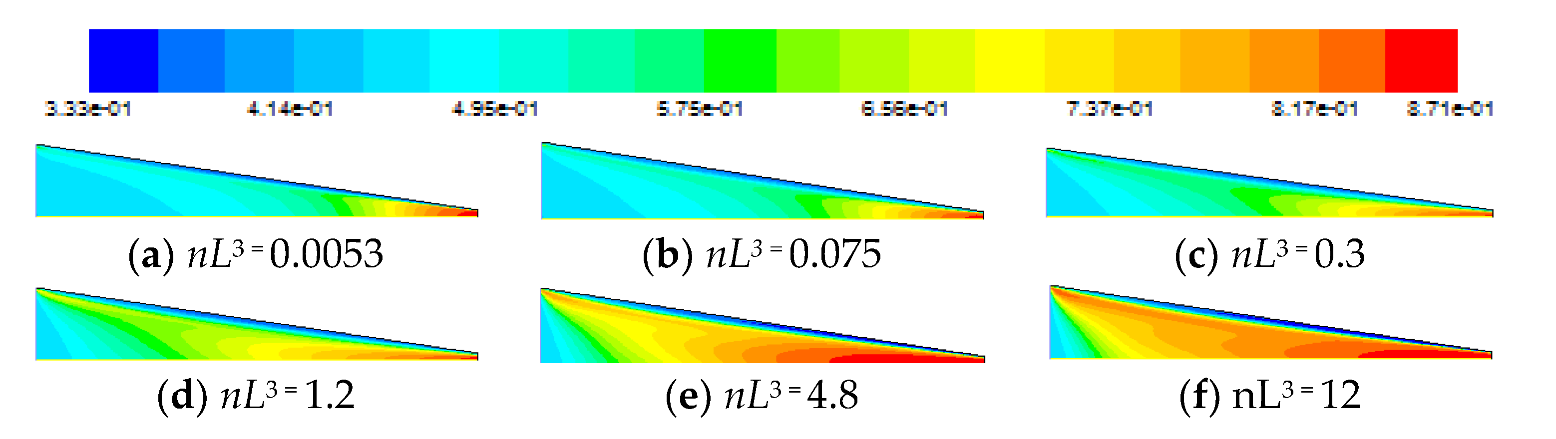
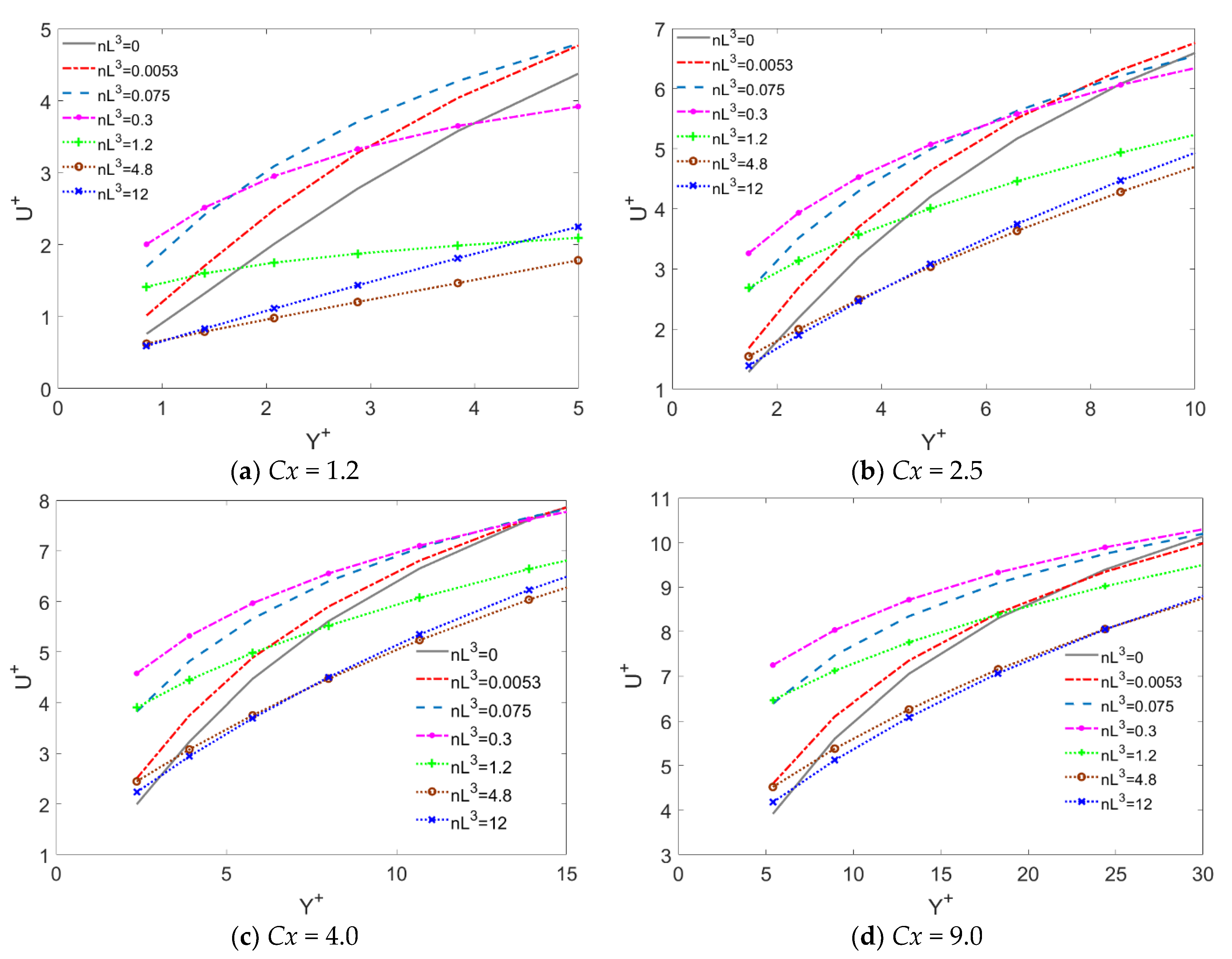
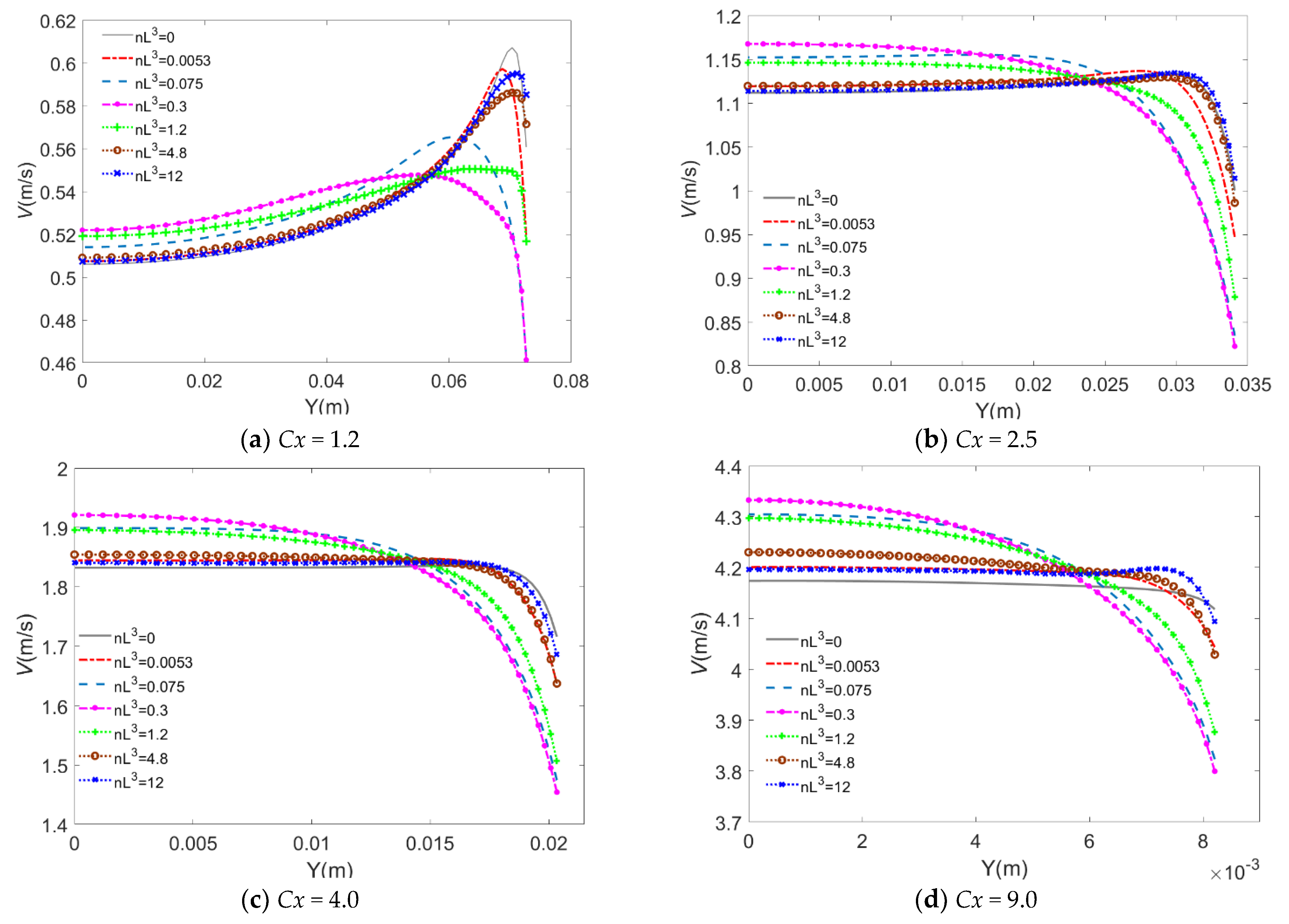
4.2. Effect of Fibers Concentrations on Suspension Flow

A wall is the main source of vorticity and turbulence in the boundary layer. The flow is basically laminar at the viscous bottom layer near the wall, so the fluid viscosity plays a decisive role in the flow transport. As shown in Figure 7 nL³ = 0.0053, nL³ = 0.075 and nL³ = 0.3 in dilute phase not only have higher wall velocity profile than that in semi-dilute phase nL³ = 1.2, nL³ = 4.8 and nL³ = 12, but also higher than that in Newtonian flow field as C_x increases. But in the complete turbulent layer and blending region, things are not the same. Turbulence is dominant in the complete turbulent layer. In the Blending region, the effects of fluid viscosity and turbulence are equivalent. The phase concentrations nL³ = 0.0053, nL³ = 4.8 and nL³ = 12 have higher wall velocity profiles than the adjacent semi-dilute phases nL³ = 0.075, nL³ = 0.3 and nL³ = 1.2. as C_x increases in the Figure 8. At the same time, the thickness of boundary layer decreases with the increase of wall shear velocity.

In the central region of turbulence, the velocity profile gradually changes from concave surface to convex surface with the increase of C_x due to the influence of contract wall, shown as Figure 9. Near the center streamline, the velocity profile of nL³ = 0.3, nL³ = 0.075 and nL³ = 1.2 is higher than that of nL³ = 0.0053, nL³ = 4.8 and nL³ = 12, but it is the opposite in the area near the wall. This may be related to the evolution of fiber orientation distribution in the flow field. When C_x > 2, fibers in the turbulent central region that are subjected to tensile effect of contract flow strongly behave the obvious alignment while fibers are randomly oriented in the boundary layer. The fibers aligned along the streamlines take advantage of the additional term of Equation (14) to make the calculated average velocity of the flow slightly higher than the original flow field without the additional term. This additional viscous action mechanism changes the velocity profile of the local suspension flow, which behaves with a certain drag reduction trend on the central turbulent region.

5. Conclusions

In order to understand the effect of fiber concentration on the average flow and fiber orientation distribution in the turbulent contraction, a coupling Euler model was used for numerical simulation. In view of the relative independence of displacement and angle space calculation, a semi-discrete approximation form is adopted to simplify the Fokker-Plank type function of fiber orientation angle. At the same time, the explicit fourth-order Runge-Kutta method is introduced to greatly reduce the iterative calculation cost. The velocity profile and fiber orientation distribution of suspension flow can be obtained under different fiber concentrations based on the Reynolds stress model solver of Fluent software.

Due to the local tensile effect in the turbulent contraction whose contract ratio C_x > 4, the higher fibers concentration is, the easier it is to move in clusters and earlier align with the flow direction when the fiber concentration exceeds the semi-dilute phase. Fibers in near semi-dilute suspension have more orientations than those in the dilute suspensions because there is hydraulic disturbance and lubrication within the range of fiber length for semi-dilute suspension.

From the mechanism of two-way coupling RSM, the fiber’s concentration mainly affects the additional stress of suspension through the additional viscosity term, and then affects the orientation diffusion of the fibers through the flow field, and finally determines the orientation distribution of fibers. Hence the addition of fibers changes the viscosity of the flow field and affects the momentum and mass transport mechanism of the suspension flow. The results of a two-way coupling simulation are basically consistent with the theory and functions of the model here, which can provide a process strategy for fiber orientation optimization and rheological control in the industrial applications of suspension such as paper making and textile.

References

1. Harris, J.B.; Pittman, J.F.T. Alignment of slender rod-like particles in suspension using converging flow. Trans. Inst. Chem. Eng. 1976, 54, 73. [Google Scholar]
2. Ullmar, M.; Norman, B. Observation of Fiber Orientation in a Headbox Nozzle at Low Consistency; TAPPI Conference Papers; TAPPI: Peachtree Corners, GA, USA, 1997; p. 865. [Google Scholar]
3. Ullmar, M. On Fiber Orientation Mechanism in a Headbox Nozzle. Licentiate Thesis, Royal Institute of Technology, Stockholm, Sweden, 1998. [Google Scholar]
4. Zhang, X. Fibre Orientation in a Headbox. Master’s Thesis, The University of British Columbia, Vancouver, BC, Canada, 2001. [Google Scholar]
5. Olson, J.A. The Motion of Fibre in turbulent flow, stochastic simulation of isotropic homogeneous turbulence. Int. J. Multiph. Flow 2001, 27, 2083–2103. [Google Scholar] [CrossRef]
6. Olson, J.A.; Frigaard, I.; Chan, C.; Hämäläinen, J.P. Modeling a turbulent fibre suspension flowing in a planar contraction: The one-dimensional headbox. Int. J. Multiph. Flow 2004, 30, 51–66. [Google Scholar] [CrossRef]
7. Parsheh, M.; Brown, M.L.; Aidun, C.K. On the orientation of stiff fibres suspended in turbulent flow in a planar contraction. J. Fluid Mech. 2005, 545, 245–269. [Google Scholar] [CrossRef]
8. Parsheh, M.; Brown, M.L.; Aidun, C.K. Variation of fiber orientation in turbulent flow inside a planar contraction with different shapes. Int. J. Multiph. Flow 2006, 32, 1354–1369. [Google Scholar] [CrossRef]
9. Lin, J.; Liang, X.; Zhang, S. Fibre Orientation Distribution in Turbulent Fibre Suspensions Flowing through an Axisymmetric Contraction. Can. J. Chem. Eng. 2011, 89, 1416–1425. [Google Scholar] [CrossRef]
10. Lin, J.; Shen, S.; Ku, X. Characteristics of Fiber Suspension Flow in a Turbulent Boundary Layer. J. Eng. Fibers Fabr. 2013, 8, 17–29. [Google Scholar] [CrossRef]
11. Wei, Y. Optimal contract wall for desired orientation of fibers and its effect on flow behavior. J. Hydrodyn. 2017, 29, 495–503. [Google Scholar]
12. Olson, J.A.; Kerekes, R.J. The motion of fibres in turbulent flow. J. Fluid Mech. 1998, 377, 47–64. [Google Scholar] [CrossRef]
13. Gillissen, J.J.J.; Boersma, B.J.; Mortensen, P.H.; Andersson, H.I. The stress generated by non-Brownian fibers in turbulent channel flow simulation. Phys. Fluids 2007, 19, 1–8. [Google Scholar] [CrossRef]
14. Johnson, T.; Röyttä, P.; Mark, A.; Edelvik, F. Simulation of the spherical orientation probability distribution of paper fibers in an entire suspension using immersed boundary methods. J. Non-Newton. Fluid Mech. 2016, 229, 1–7. [Google Scholar] [CrossRef]
15. Lin, J.Z.; Zhang, L.X.; Zhang, W.F. Rheological Behavior of Fiber Suspensions in a Turbulent Channel Flow. J. Colloid Interface Sci. 2006, 296, 721–728. [Google Scholar] [CrossRef] [PubMed]
16. Lin, J.Z.; Zhang, S.L.; Olson, J.A. Effect of Fibers on the Flow Property of Turbulent Fiber Suspensions in a Contraction. Fibers Polym. 2007, 8, 60–65. [Google Scholar] [CrossRef]
17. Lin, W.; Shi, R.; Lin, J. Distribution and Deposition of Cylindrical Nanoparticles in a Turbulent Pipe Flow. Appl. Sci. 2021, 11, 962. [Google Scholar] [CrossRef]
18. Yang, W.; Zhou, K.; Zhao, Z.L.; Wan, Z.H. Study on the two-way coupling turbulent model and rheological properties for fiber suspension in the contraction. J. Non-Newton. Fluid Mech. 2017, 246, 1–9. [Google Scholar] [CrossRef]
19. Batchelor, G.K. Slender-body theory for particles of arbitrary cross-section in stokes flow. J. Fluid Mech. 1970, 44, 419–440. [Google Scholar] [CrossRef]
Figure 1. Two-dimension model of contraction.
Applsci 11 07126 g001
Figure 2. Comparison of consequences at the center streamline by Parsheh’s experiments, one-way and two-way simulation.
Applsci 11 07126 g002
Figure 3. a1111 distribution in the contract flow at different nL3.
Applsci 11 07126 g003
Figure 4. Probability distribution f(φ) of fibers orientation angleφ varying with nL3 in the contraction where (a) nL3 = 0.0053, (b) nL3 = 0.075, (c) nL3 = 0.3, (d) nL3 = 1.2, (e) nL3 = 4.8, (f) nL3 = 12.
Applsci 11 07126 g004
Figure 5. a1111 varying with Y+ from the wall to the boundary layer at different nL3.
Applsci 11 07126 g005
Figure 6. a1111 varying with Y from the central streamline to near-wall area at different nL3.
Applsci 11 07126 g006
Figure 7. U+ varying with Y+ from the wall to the viscous bottom layer at different nL3.
Applsci 11 07126 g007
Figure 8. U+ varying with Y+ from the wall to the boundary layer at different nL3.
Applsci 11 07126 g008aApplsci 11 07126 g008b
Figure 9. a1111 varying with Y from the central streamline to near-wall area at different nL3.
Applsci 11 07126 g009