An Algorithm for Solving Robot Inverse Kinematics Based on FOA Optimized BP Neural Network

Abstract

The solution of robot inverse kinematics has a direct impact on the control accuracy of the robot. Conventional inverse kinematics solution methods, such as numerical solution, algebraic solution, and geometric solution, have insufficient solution speed and solution accuracy, and the solution process is complicated. Due to the mapping ability of the neural network, the use of neural networks to solve robot inverse kinematics problems has attracted widespread attention. However, it has slow convergence speed and low accuracy. This paper proposes the FOA optimized BP neural network algorithm to solve inverse kinematics. It overcomes the shortcomings of low convergence accuracy, slow convergence speed, and easy to fall into local minima when using BP neural network to solve inverse kinematics. The experimental results show that using the trained FOA optimized BP neural network to solve the inverse kinematics, the maximum error range of the output joint angle is [−0.04686, 0.1271]. The output error of the FOA optimized BP neural network algorithm is smaller than that of the ordinary BP neural network algorithm and the PSO optimized BP neural network algorithm. Using the FOA optimized BP neural network algorithm to solve the robot kinematics can improve the control accuracy of the robot.

1. Introduction

Solving the problem of robot inverse kinematics is the basis of robot trajectory planning and motion control. Inverse kinematics is the mapping from Cartesian space to joint space [1,2]. Its essence is to obtain the value of each joint variable from the position and posture of the end of the robot. Traditional methods for solving robot inverse kinematics include geometric [3,4], algebraic [5,6,7], and iterative [8,9] methods. The geometric method has strict requirements on the configuration of the robot, poor versatility, certain limitations, and the modeling and solving process is more complicated. The algebraic method can obtain closed solutions of simple mechanisms. However, it is difficult to obtain closed solutions of complex mechanisms. This method involves a quantity of coordinate transformations in the solution process, and the solution accuracy is relatively low. The iterative method solves the problem through repeated iterations. This method requires numerous calculations and is difficult to meet the requirements of real-time control.

In view of the shortcomings of traditional methods, more and more intelligent algorithms are widely used in robot control, such as neural network algorithms [10,11], genetic algorithms [12,13,14,15], and particle swarm algorithms [15,16,17,18]. Artificial neural network has powerful approximation ability when solving the problem of nonlinear mapping. Taking a large number of positive kinematics information of the robot as samples, through the training and learning of the BP neural network, the mapping from the Cartesian space to the joint space is realized. As a result, complicated calculation and derivation processes are avoided. The trained neural network has a fast calculation speed and can meet the requirements of real-time control.

In [19], Karlik and Aydin proved that the double hidden layer BP neural network structure has advantages in solving the inverse kinematics of the manipulator. However, the traditional BP neural network has the disadvantages of large output error, easy to fall into a local extreme value, and slow convergence speed. In [15], Mustafa et al. designed two scenarios of randomly selected points and following a specific trajectory in the robot workspace, compared four different optimization algorithms, and proved the effectiveness of the QPSO algorithm to solve the inverse kinematics of a 4-DOF serial robot. Ozgoren [20] used the analytical method to solve the inverse kinematics of the redundant manipulator and optimized it accordingly, but the solution process was complicated, and the solution accuracy was not high.

In [21], Dereli et al. proposed global-local best inertia PSO algorithm and proved the effectiveness of the PSO algorithm in solving the optimal solution of redundant robots. Ren and Ben-Tzvi [22] proposed a series of improved GANs that use limited data to approximate the real model, effectively solving the inverse kinematics problem of high-dimensional nonlinear systems. Dereli and Köker [23] proposed using the firefly algorithm to solve the inverse kinematics of a 7-DOF robot, but the population size has a great influence on the speed and quality of the solution. In [24], Zhou et al. proposed an intelligent algorithm that initializes the inverse kinematics solution with extreme learning machine and optimizes it with a genetic algorithm based on sequence mutation. This algorithm improves the efficiency of the solution while ensuring accuracy.

Fruit fly optimization algorithm has few applications in the field of robot kinematics [25,26,27,28]. The FOA algorithm has the characteristics of simple operation and fast convergence speed. This paper uses the FOA algorithm to optimize the threshold and weight of the BP neural network to improve the convergence speed and output accuracy of the neural network. The optimized neural network is used to solve the inverse kinematics of the robot shown in Figure 1, and compared with the ordinary BP neural network algorithm and the PSO optimized BP neural network algorithm. The robot structure shown in Figure 1 is a part of the service robot. It can be installed on a mobile chassis with laser radar [29] and equipped with robotic arms to form a complete service robot.

This paper proposes an FOA optimized BP neural network algorithm to improve the accuracy of solving robot inverse kinematics. This paper is organized as follows: In Section 2, the robot kinematics model is established. In Section 3, the FOA optimized BP neural network algorithm is introduced. The distance and direction of the individual in the FOA algorithm are regarded as the threshold and weight of the neural network for iterative optimization. In Section 4, the proposed FOA optimized BP neural network is compared with the ordinary BP neural network and the PSO optimized BP neural network, and the error of the inverse kinematics of the robot is compared. In Section 5, the results show that the FOA optimized BP neural network algorithm can improve the accuracy of solving robot inverse kinematics.

2. Robot Kinematics

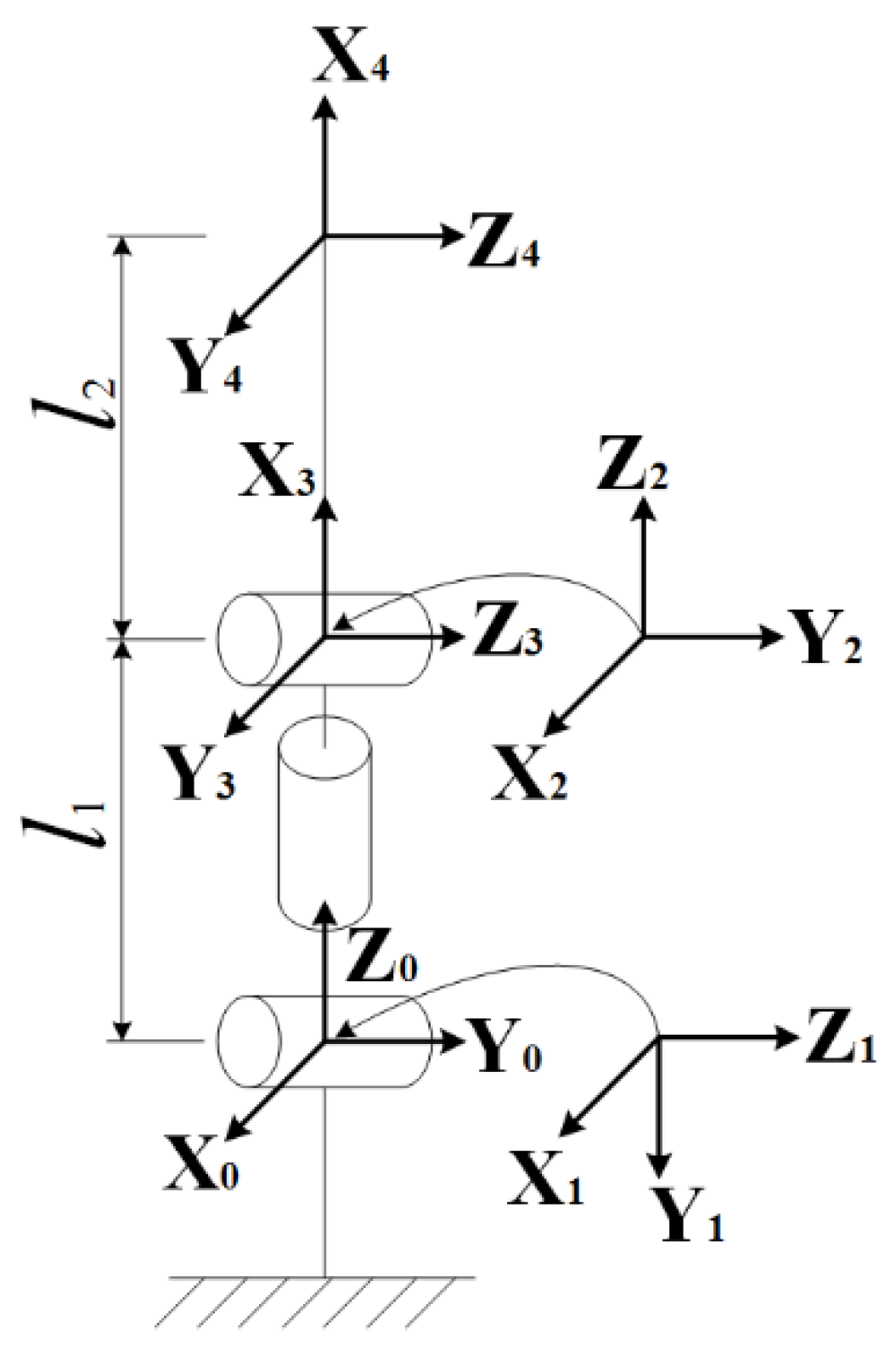
The robot torso coordinate system is established according to the D-H method, as shown in Figure 2.

The system has four linkages and five coordinate systems. Here, α_i, a_i, $d_i$, and ${\theta }_i$ respectively represent the connecting rod torsion angle, connecting rod length, connecting rod offset, and joint angle. According to the built robot kinematics model,

Table 1. Link parameters of the robot.

i	αi−1 (rad)	ai−1 (mm)	di (mm)	θi (rad)
1	−π/2	0	0	θ1
2	π/2	0	l1	θ2
3	−π/2	0	0	θ3 − π
4	0	l2	0	0

shows the link parameters of the robot.

After defining the linkage coordinate system and the corresponding linkage parameters, the kinematic equation can be established. The D-H transformation matrix ${}_i{}^{i-1}T$ can be obtained by right multiplying the following four transformation matrices:

$$\begin{array}{ll}{}_i{}^{i-1}T& =R_x({\alpha }_{i-1})D_x(a_{i-1})R_z({\theta }_i)D_z(d_i)\\ & =\left[\begin{array}{cccc}c{\theta }_i& -s{\theta }_i& 0& a_{i-1}\\ s{\theta }_{i}c{\alpha }_{i-1}& c{\theta }_{i}c{\alpha }_{i-1}& -s{\alpha }_{i-1}& -s{\alpha }_{i-1}{d}_i\\ s{\theta }_{i}s{\alpha }_{i-1}& c{\theta }_{i}s{\alpha }_{i-1}& c{\alpha }_{i-1}& c{\alpha }_{i-1}{d}_i\\ 0& 0& 0& 1\end{array}\right]\end{array}$$

(1)

where ${}_i{}^{i-1}T$ is the D-H transformation matrix transformed from coordinate system i to i − 1, $R_x({\alpha }_{i-1})$ is the rotation matrix representing a rotation of α_i−1 around the X axis, $D_x(a_{i-1})$ is the translation matrix representing a translation of a_i−1 along the X axis, $R_z({\theta }_i)$ is the rotation matrix representing a rotation of ${\theta }_i$ around the Z axis, $D_z(d_i)$ is the translation matrix representing a translation of $d_i$ around the Z axis, $c{\theta }_i$ is short for $\cos {\theta }_i$, $s{\theta }_i$ is short for $\sin {\theta }_i$, etc. The transformation matrices of each link determined by the link parameters are multiplied to obtain the position and posture of the center point of the robot’s chest in the base coordinate system:

$${}_4{}^{0}T={}_1{}^{0}T{}_2{}^{1}T{}_3{}^{2}T{}_4{}^{3}T=\left[\begin{array}{cc}{}_4{}^{0}R{}_{3\times 3}& {}_4{}^{0}P{}_{3\times 1}\\ 0& 1\end{array}\right]=\left[\begin{array}{cccc}{r}_{11}& r_{12}& r_{13}& p_x\\ r_{21}& r_{22}& r_{23}& p_y\\ r_{31}& r_{32}& r_{33}& p_z\\ 0& 0& 0& 1\end{array}\right]$$

(2)

where ${}_4{}^{0}R{}_{3\times 3}$ is the rotation transformation matrix transformed from coordinate system 4 to 0, ${}_4{}^{0}P{}_{3\times 1}$ is the position vector transformed from coordinate system 4 to 0, $r_{ij}$ is the element of ${}_4{}^{0}R{}_{3\times 3}$, and $p_x$, $p_y$, $p_y$ is the component of the translation vector ${}_4{}^{0}P{}_{3\times 1}$.

The rotation matrix ${}_4{}^{0}R{}_{3\times 3}$ can be described by rotating around the axis of a fixed reference coordinate system, as shown in Formula (3):

$${}_4{}^{0}R{}_{XYZ}(\gamma ,\beta ,\alpha )=\left[\begin{array}{ccc}c\alpha c\beta & c\alpha s\beta s\gamma -s\alpha c\gamma & c\alpha s\beta c\gamma +s\alpha s\gamma \\ s\alpha c\beta & s\alpha s\beta s\gamma +c\alpha c\gamma & s\alpha s\beta c\gamma -c\alpha s\gamma \\ -s\beta & c\beta s\gamma & c\beta c\gamma \end{array}\right]$$

(3)

where ${}_4{}^{0}R{}_{XYZ}(\gamma ,\beta ,\alpha )$ is the equivalent rotation matrix that rotates $\gamma$, $\beta$, and $\alpha$ around the X, Y, and Z axes of the fixed reference coordinate system.

Equivalently derived X-Y-Z fixed angle from the rotation matrix:

$$\begin{array}{l}\beta =\mathrm{Atan}2(-r_{31},\sqrt{r_{11}^2+r_{21}^2})\\ \alpha =\mathrm{Atan}2(r_{21}/c\beta ,r_{11}/c\beta )\\ \gamma =\mathrm{Atan}2(r_{32}/c\beta ,r_{33}/c\beta )\end{array}$$

(4)

where $\mathrm{Atan}2(y,x)$ is the arctangent function of a two-parameter variable.

These equations can provide the pose of the robot relative to the world coordinate system. The forward kinematics equation of the robot can be expressed as:

$${\mathrm{F}}_{\mathrm{forword} \mathrm{kinematics}}({\theta }_1,{\theta }_2,{\theta }_3) = (p_x,p_y,p_z,\alpha ,\beta ,\gamma )$$

(5)

As shown in Equation (5), the end pose of the robot can be obtained through the joint variables of the robot. However, in practical applications, it is often necessary to obtain the joint angles of the robot through the end pose of the robot, so the robot inverse kinematics is solved by the formula:

$${\mathrm{F}}_{\mathrm{inverse} \mathrm{kinematics}}(p_x,p_y,p_z,\alpha ,\beta ,\gamma ) = ({\theta }_1,{\theta }_2,{\theta }_3)$$

(6)

In order to avoid the complicated process of solving robot inverse kinematics, this paper proposes an FOA optimized BP algorithm. The BP neural network is used to fit Equation (5). The fruit fly optimization algorithm is used to optimize the initial weights and thresholds of the BP neural network to improve the global optimization ability of the neural network. The data set is used to continuously train the FOA optimized BP neural network to find the optimal neural network. Finally, the optimal network is used to solve the robot inverse kinematics. The model of the algorithm is shown in Figure 3.

3. Algorithm Principle

3.1. BP Neural Network Algorithm

In 1985, the scholars Rumelhart and McCelland proposed a multi-layer feedforward artificial neural network using the error back propagation algorithm, namely BP neural network [30]. The ordinary BP neural network contains two parts: the forward propagation of the signal and the back propagation of the error. The actual output is calculated from the input to the output, and weights and thresholds are corrected from the output to the input. A single basic artificial neuron model is shown in Figure 4.

Among them, $x_j(j=1,2,\cdots ,N)$ is the input of the j-th node, $w_{ij}$ is the weight, ${\theta }_i$ is the threshold, and $y_i$ is the output of neuron i. The output $y_i$ can be expressed as:

$$y_i=f({\mathrm{net}}_i)=f({\displaystyle \sum _{j=1}^N{w}_{ij}{x}_j+{\theta }_i})$$

(7)

Among them, the f function is the activation function, and the most commonly used form is the Sigmoid function, and its expression is Formula (8):

$$f(x)=\frac{1}{1+e^{-ax}},a\in \mathrm{C}$$

(8)

If the net activation f is positive, the neuron is in an excited state. Otherwise, the neuron is in a suppressed state.

This paper uses the BP algorithm to solve inverse kinematics. A neural network structure is established, and the input layer has six input signals, corresponding to $p_x$, $p_y$, $p_z$, $\alpha$, $\beta$, $\gamma$. The output layer has three output signals, respectively, corresponding to the robot’s three joints ${\theta }_1$, ${\theta }_2$, ${\theta }_3$.

According to Kolmogorov’s theorem, a BP neural network with one hidden layer can complete any n-dimensional to m-dimensional mapping [31]. Increasing the number of layers of the neural network can improve the accuracy. However, it will complicate the neural network and extend the training time. Using two hidden layers can make the mapping effect of the neural network better, and increasing the number of neurons in the hidden layer can improve the accuracy. In the BP neural network, the number of neurons in each layer has a great influence on the network performance. According to Equation (6), after experiments and comparisons, this paper chooses a network structure containing two hidden layers. The first hidden layer has 24 neurons, and the second hidden layer has 43 neurons. The designed BP neural network topology is shown in Figure 5.

Figure 5 shows the topology of the designed BP neural network. The layers are fully interconnected, and there is no interconnection between the same layers.

The core of the BP neural network algorithm is to solve the minimum value of the error function. BP neural network adjusts the weights and thresholds of each layer according to the error gradient descent method. There are weaknesses, such as slow convergence, low learning efficiency, weak generalization ability, and easy to fall into local minimums. Therefore, the optimization algorithm is combined for improvement.

3.2. Fruit Fly Optimization Algorithm

The scholar Pan Wenchao proposed a fruit fly optimization algorithm after long-term observation of fruit flies [32]. Compared with other organisms, fruit flies have a particularly sensitive sense of vision and smell. During their activities, fruit flies perceive the taste of food through smell, and use their unique vision to move in the direction where other fruit flies gather.

The fruit fly optimization algorithm is to find the global optimum through the foraging evolution of Drosophila fruit flies. Foraging for fruit flies is divided into two procedures. The first procedure is relying on a strong sense of smell to initially locate the food source and quickly approach the food source; the second procedure is discovering where food and companions gather through vision and fly in that direction. The basic optimization process of the fruit fly optimization algorithm is the fruit fly population starts from a given initial position, and performs an olfactory search according to the given flight direction and step distance. Then, the approximate direction of the optimal solution and the distance between the fruit fly and the optimal solution are preliminarily determined by the concentration, and finally the position of the optimal solution is reached through visual search. The fruit fly optimization algorithm has a good global optimization ability, and can meet the optimization problems in different fields.

According to the foraging process of fruit flies, the fruit fly algorithm performs optimization according to the following necessary steps:

• Set the size of the fruit fly population and initialize the position of the fruit fly population randomly;
• Set the direction and distance for individual fruit flies to search randomly through smell:

  $$\begin{array}{l}{X}_i=X_{axis}+\mathrm{RandomValue}\\ Y_i=Y_{axis}+\mathrm{RandomValue}\end{array}$$

  (9)
• The location of the food is unknown. First, calculate the distance D(i) from the origin, and use the reciprocal of the distance D(i) as the taste concentration judgment value S(i):

  $$\begin{array}{l}D(i)=\sqrt{X_i^2+Y_i^2}\\ S(i)=1/D(i)\end{array}$$

  (10)
• Substitute S(i) into the taste concentration judgment function fitness, the taste concentration Smell(i) at the individual position of the fruit fly can be obtained:

  $$Smell(i)=\mathrm{Fitness}(S(i))$$

  (11)
• Find the fruit fly with the best taste concentration Smell in the population:

  $$[bestSmell,bestindex] = \mathrm{minimum}(Smell)$$

  (12)
• Keep the X and Y coordinates of the best individual fruit fly, and the best taste concentration value;
• Repeat steps (2) to (5) for iterative optimization, and judge whether the taste concentration of the current iteration is better than that of the previous iteration, and if so, proceed to the next iteration after step (6).

3.3. FOA Optimized BP Algorithm

In order to make up for the shortcomings of the BP algorithm, this paper uses the FOA algorithm to optimize the parameters of the BP algorithm and improve the generalization ability and output accuracy of the BP algorithm. The algorithm flow is shown in Figure 6.

According to Equation (6), $p_x, p_y, p_z, \alpha , \beta , \gamma$ are input, and ${\theta }_1, {\theta }_2, {\theta }_3$ are output. A BP neural network structure is constructed with six inputs and three outputs. The input and output samples are normalized. The initial weight and initial threshold of the neural network are randomly generated. In the FOA optimized BP neural network algorithm, the initial weights and initial thresholds are used as the initial position of the fruit fly. The seven steps of the fruit fly optimization algorithm are followed, the value of the corresponding fitness calculated, and then the optimal weight and threshold are found through iteration. Among them, the fitness function is represented by the variance function of the joint angle output by the BP and the expected joint angle, expressed as:

$$J(k) = \frac{1}{N}{\displaystyle \sum _{i=1}^N{({\theta }_i(k) - {\theta }_i)}^2}$$

(13)

where N represents the number of training samples, ${\theta }_i(k)$ represents the output of the i-th sample at the k-th iteration, and ${\theta }_i$ represents the expected output value of the i-th sample.

The optimal weights and thresholds found by the fruit fly optimization algorithm are used as the initial weights and initial thresholds of the BP algorithm to train the neural network. Finally, the trained neural network is used to solve the inverse kinematics. In the FOA optimized BP algorithm, the fruit fly population size is set to 30 and set up to 50 iterations.

The FOA optimized BP algorithm uses the FOA algorithm to find the global optimum, and the BP algorithm to find the local optimum. The algorithm’s convergence speed, generalization ability, and convergence accuracy are improved.

4. Simulation and Discussion

In the simulation experiment, based on the Monte Carlo method, 2000 sets of samples are generated in the robot workspace, of which 1950 sets are used as training samples and 50 sets are used as test samples. The robot end position coordinates and fixed angle samples in the training samples are used as the input of the BP neural network, and the joint angle samples of the robot are used as the output of the BP neural network. Then, theFOA algorithm is used to optimize the convergence of the network, and the weights and thresholds of the BP neural network are returned. The training samples are brought into the FOA optimized BP algorithm to train the network. Finally, the test samples are brought into the trained network for testing, and the joint variables of the robot outputted by the test samples are obtained.

The FOA optimized BP algorithm contains two hidden layers. The first hidden layer has 24 neurons and the second hidden layer has 43 neurons. The number of fruit flies is set to 30, and the number of iterations is set to 50. In order to intuitively reflect the effect of the algorithm proposed in this article, the FOA optimized BP algorithm is compared with the ordinary BP algorithm and the PSO optimized BP algorithm. In the PSO optimized BP algorithm, the number of particles is set to 30, and 50 iterations are set. The learning factor $c_1=c_2=2$, and the inertia factor $w=0.95$, are used.

After the simulation, the robot joint variables output by the three algorithms are compared with the expected values in the test samples.

Table 2. The range of joint error and the range of MSE.

Joint Error and MSE	BP	PSO-BP	FOA-BP
$\Delta {\theta }_1(°)$	−0.1530–0.1775	−0.07472–0.07594	−0.02583–0.03612
$\Delta {\theta }_2(°)$	−0.2723–0.2977	−0.1570–0.2022	−0.04686–0.1271
$\Delta {\theta }_3(°)$	−0.11206–0.2087	−0.07277–0.1599	−0.02986–0.03678
MSE	6.400 × 10−6–1.983 × 10−3	6.390 × 10−6–1.116 × 10−3	2.870 × 10−7–3.258 × 10−4

shows the maximum error range and the overall mean square error (MSE) range of each joint in the 50 groups of samples.

From the results in Table 2, it can be seen that the maximum error range of the joint variables output by the ordinary BP algorithm is [−0.2723, 0.2977], and the range of MSE is [6.400 × 10⁻⁶, 1.983 × 10⁻³]. The maximum error range of the joint variables output by the PSO optimized BP algorithm is [−0.1570, 0.2022], and the range of MSE is [6.390 × 10⁻⁶, 1.116 × 10⁻³]. The maximum error range of the joint variables output by the FOA optimized BP algorithm is [−0.04686, 0.1271], and the range of MSE is [2.870 × 10⁻⁷, 3.258 × 10⁻⁴]. Figure 7, Figure 8 and Figure 9 show the comparison of the errors of each joint output by the three algorithms for 50 sets of samples. Figure 10 is a comparison of the MSE output by the three algorithms.

It can be seen from Figure 7, Figure 8 and Figure 9 that the output error of the ordinary BP algorithm is the largest, and the output error of the FOA optimized BP algorithm is the smallest. The error distribution of the FOA optimized BP algorithm is relatively uniform. From Figure 10, it can be seen that the MSE output by the FOA optimized BP algorithm is much smaller than the MSE output by the other two algorithms.

It can be seen that when solving the robot inverse kinematics, the error of the FOA optimized BP algorithm is smaller than that of the ordinary BP algorithm and PSO optimized BP algorithm, and the MSE is also significantly reduced. The FOA optimized BP algorithm can improve the accuracy of solving inverse kinematics. The effectiveness of the FOA optimized BP algorithm in solving the inverse kinematics of the robot is verified.

5. Conclusions

This paper proposes an FOA optimized BP algorithm to solve the robot inverse kinematics. The nonlinear mapping ability of the BP neural network was used to avoid the complicated derivation process of solving robot inverse kinematics. Using the characteristics of the fruit fly optimization algorithm, the convergence accuracy, convergence speed, and generalization ability of BP algorithm were improved. The proposed FOA optimized BP algorithm can significantly improve the problems of complex calculations, large calculations, and difficult-to-guarantee accuracy in other robot inverse kinematics solving methods. The experimental results prove that the error of the FOA optimized BP algorithm is obviously smaller than that of the ordinary BP algorithm and the PSO optimized BP algorithm. After obtaining a large amount of experimental data, the positioning accuracy of the robot can be improved, which has important application value.