Featured Application
This work was supported by the National Nature Science Foundation of China (No. 52075468; No. 52005428); General project of Natural Science Foundation of Hebei Province (No. E2020203052; No. 2021203099); Youth Fund Project of a scientific research project of Hebei University (No. QN202013).
Abstract
Magnetic liquid double suspension bearing (MLDSB) is composed of an electromagnetic system and hydrostatic system and its bearing capacity and stiffness can be greatly improved. It is very suitable for occasions of medium speed, heavy load, and starting frequently. Due to the gyroscopic effect and interference between the supporting system, the space state of the rotor can be affected and the operation stability of the MLDSB can be reduced greatly. Therefore, the coupling features of the multi-degree of freedom (multi-DOF) system are analyzed and a decoupling controller is designed and verified in the paper. Firstly, the paper introduces the structural characteristics, stress forms, and control regulation mechanism. Then, the mathematical transfer function of the multi-DOF supporting system is established and the coupling principle is revealed. The state feedback decoupling controller is designed by means of a state feedback decoupling, and its decoupling effect is analyzed by the Simulink module. Finally, the single-DOF decoupling system is independently controlled by the use of the root locus method. The coupling characteristics between channel x and channel y are tested experimentally, and the decoupling controller is added and its effect tested. The results show that the state feedback decoupling controller can effectively reduce the coupling degree in the multi-DOF system and convert the multi-DOF coupling problem into a single-DOF independent control problem. The coupling effect of channel x and channel y is reduced by using the decoupling controller, with the subsequent displacement characteristic of the rotor increased, and then the operation stability of the MLDSB is improved greatly. This paper can enrich the support system of the MLDSB and provide a theoretical reference for stability control.
1. Introduction
The high-pressure desalination pump is the core power equipment that provides the reverse osmosis pressure and the flow in the reverse osmosis desalination process. As the “heart” of the reverse osmosis desalination project, it directly affects the energy consumption and operational reliability of the reverse osmosis desalination process. The reverse osmosis desalination process is shown in Figure 1.
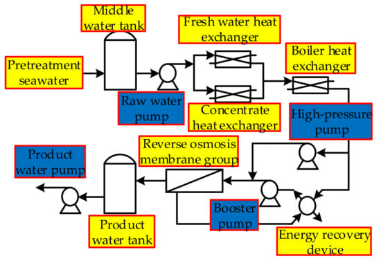
Figure 1.
Process of reverse osmosis seawater desalination.
With the rapid development of the social economy and the continuous increase of population, the lack of freshwater resources has become more and more serious, forcing seawater desalination projects to gradually develop in the direction of high power and large-scale [1].
The bearing system is a key core component to ensure the supporting performance and operational stability of the seawater desalination high-pressure pump, which directly affects the operation status, maintenance period, and service life. At present, the high-pressure pumps of medium and large seawater desalination projects are all multi-stage centrifugal pumps, which are supported by sliding bearings that use seawater as the lubricating medium. However, due to the low viscosity and special physical and chemical properties of seawater, it is difficult to form the lubricating film of seawater-lubricated friction bearings, and the supporting capacity and stiffness of liquid film are poor, which has become one of the common problems in this field [2].
To sum up, based on former research and experience, the theory of electromagnetic levitation was introduced into the seawater lubricated bearing to form a magnetic liquid double suspension bearing (MLDSB), which is suitable for a seawater desalination high-pressure pump.
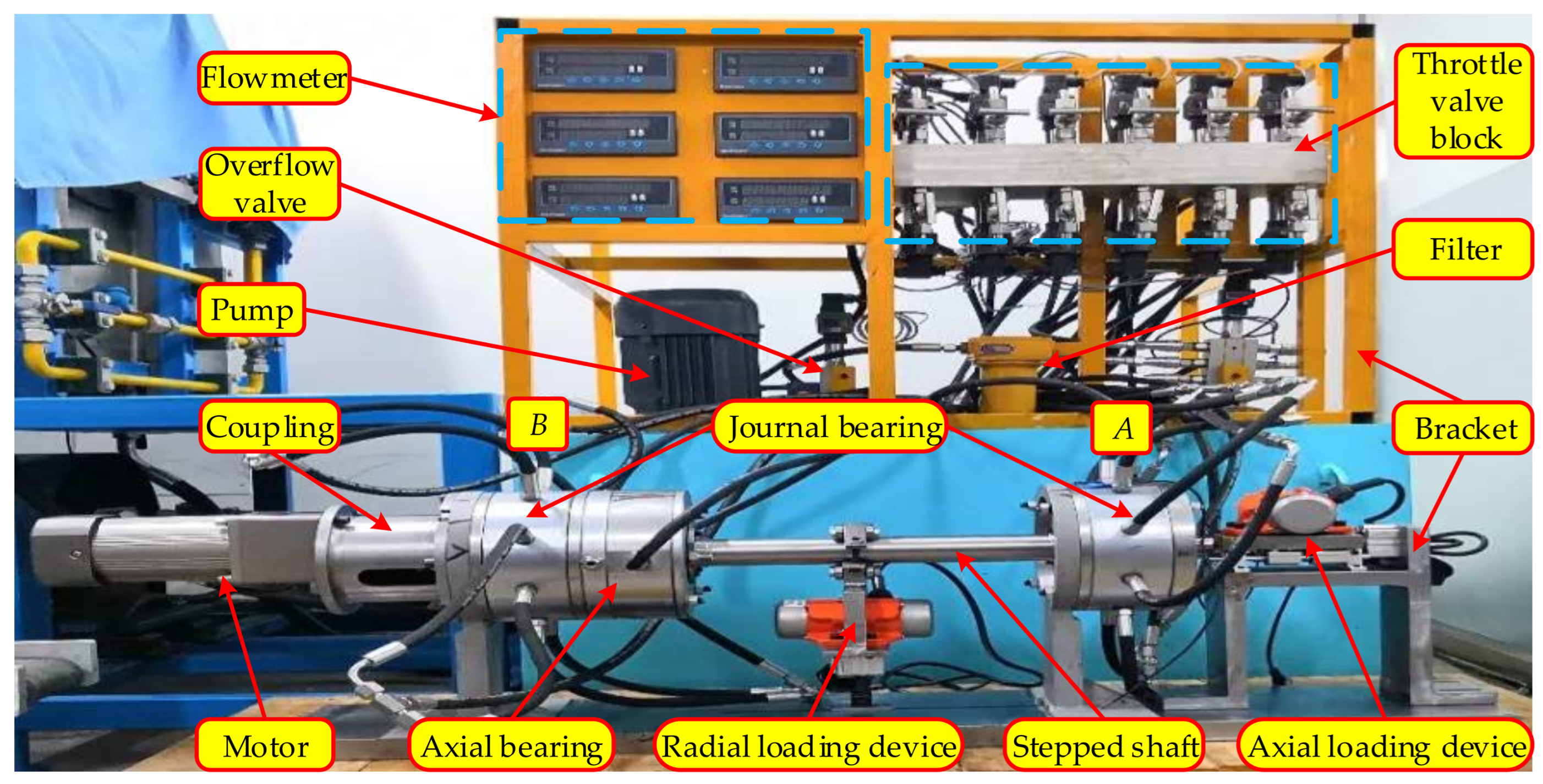
The MLDSB Experimental Table shown in Figure 2, includes the axial loading rig, radial loading rig, radial unit, composite unit, and coupling, etc.

Figure 2.
Magnetic liquid double suspension bearing (MLDSB) experimental table.
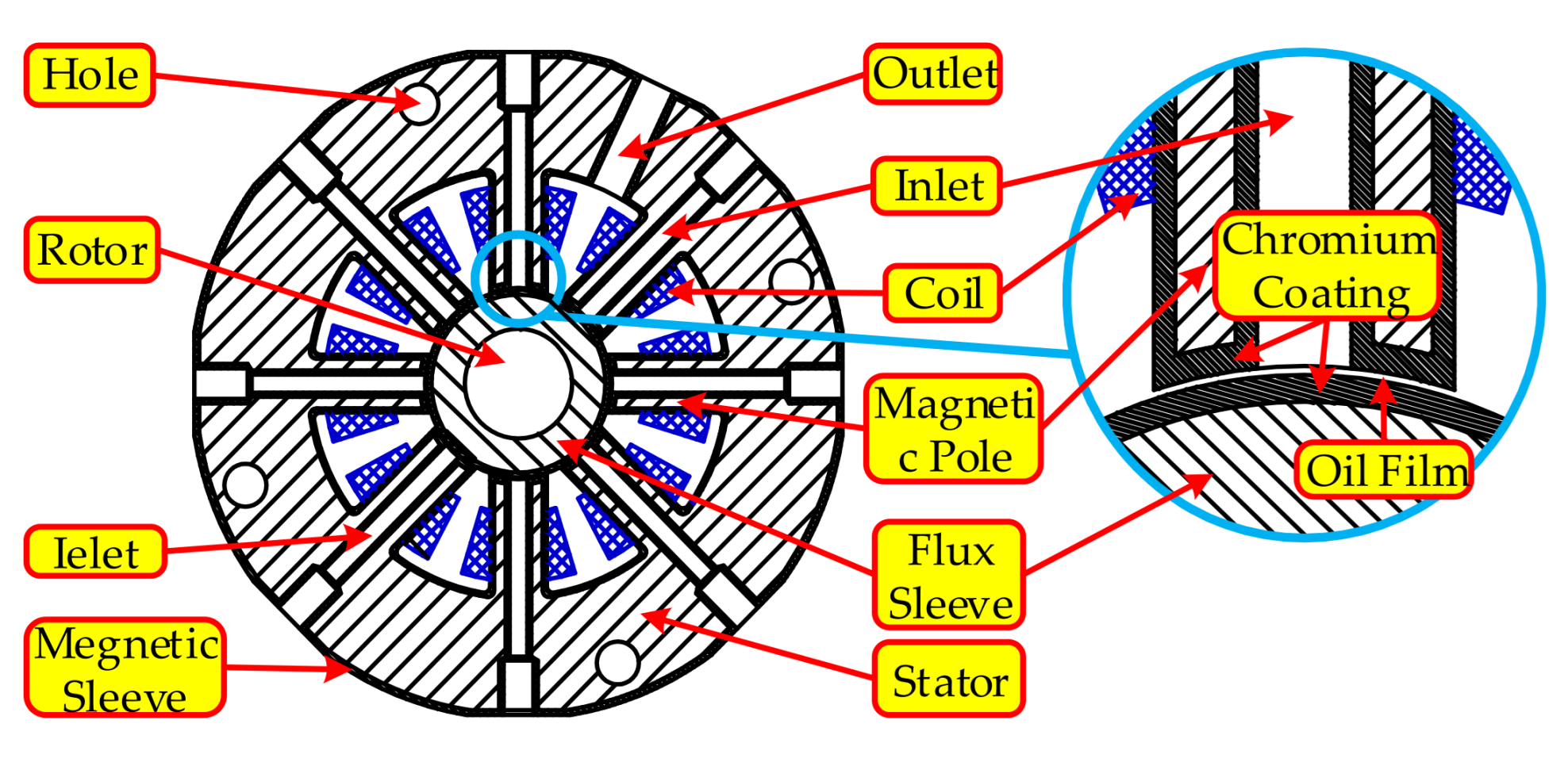
The MLDSB is mainly composed of a stator, coil, rotor, magnetic sleeve, and other components. The stator has eight circumferential magnetic poles. The coil that is arranged on the magnetic pole can make the magnetic pole produce electromagnetic force after electrifying, and the oil between the supporting cavity and magnetic conducting sleeve provide hydrostatic force [3]. The structure of the radial unit is shown in Figure 3 and Figure 4.
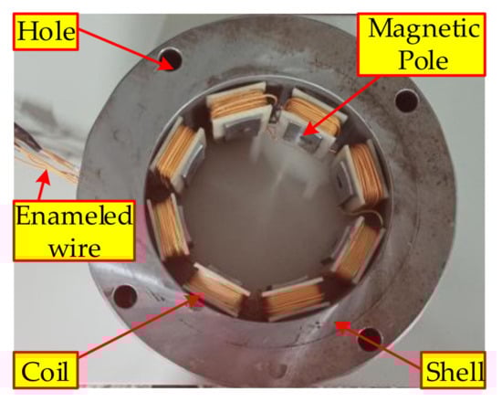
Figure 3.
Photo of the radial unit.
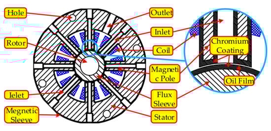
Figure 4.
Structure of the radial unit.
Due to the coupling between each magnetic pole and between the hydrostatic system and the electromagnetic system, the stability and reliability of the MLDSB can be reduced greatly [4].
As one of the most popular research topics, multi-DOF coupling characteristics of electromagnetic bearings have been studied deeply by researchers in many countries obtaining valuable results.
Focusing on the problem of electromagnetic force coupling between two DOF of a four-pole permanent magnet offset radial magnetic bearing, the causes of coupling were studied, and the feedforward decoupling control strategy and the decoupling algorithm of the feedforward compensator for the permanent magnet offset radial magnetic bearing was reviewed in the literature [5]. The comparison between the electromagnetic force and the control current before and after decoupling shows that the proposed feedforward compensation decoupling algorithm was feasible.
The literature [6] proposed a feedforward decoupling control strategy of radial four degrees of freedom for the rigid rotor system of the electromagnetic bearing. The simulation and experimental results showed that the proposed feedforward decoupling controller can decouple the original radial coupling of the rigid rotor system of the electromagnetic bearing from a four-DOF system to a four single-DOF system.
The literature [7] proposed a method based on inverse system decoupling that improved the two-DOF control. The results showed that the control algorithm can make the flywheel rotor suspend more stable and effectively suppress its vibration.
In the literature [8], complete decoupling control of the current loop cannot be achieved when the parameters are mismatched, and the decoupling effect of the current loop was not good. A control strategy of introducing a disturbance observer on the basis of deviation decoupling control was presented. The results showed that the current loop can be completely decoupled.
To sum up, the research achievements of domestic and foreign scholars are mainly focused on the coupling effect of electromagnetic or static pressure. At present, there is no research report on the decoupling control of the MLDSB with a multi-DOF. Decoupling control is the basic premise and inner core of the stable support and operation of the MLDSB. Therefore, this paper intends to establish the dynamic function of a multi-DOF supporting system, reveal the spatial coupling laws, and design a decoupling controller that will provide a theoretical reference for the stability study of the MLDSB.
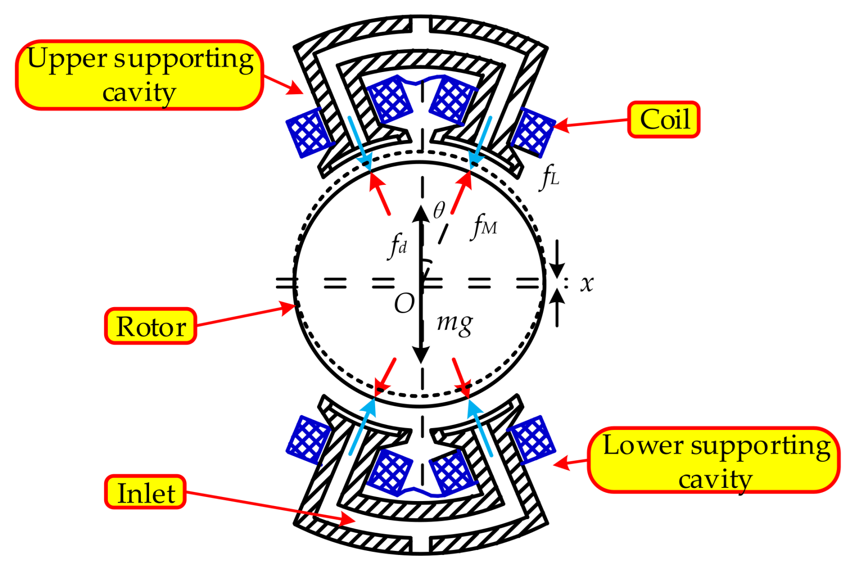
2. Regulating Principle of the Single-DOF Supporting System
The adjustment principle of the radial single-DOF supporting system is shown in Figure 5. At the initial equilibrium state, the upper/lower supporting pockets adopt a constant pressure supply model and the upper/lower electromagnetic coils adopt a differential current control model. So the electromagnetic force of the upper/lower adjacent opposite poles is the same, and then the gravity of the rotor can be balanced by the hydrostatic force of the upper/lower adjacent pockets. The two adjacent magnetic poles/pockets are called the supporting unit [9].
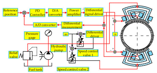
Figure 5.
Regulating principle of the radial single-DOF system.
The single-DOF supporting system of the MLDSB is composed of two upper and lower supporting units and the rotor. The structure diagram is shown in Figure 6.
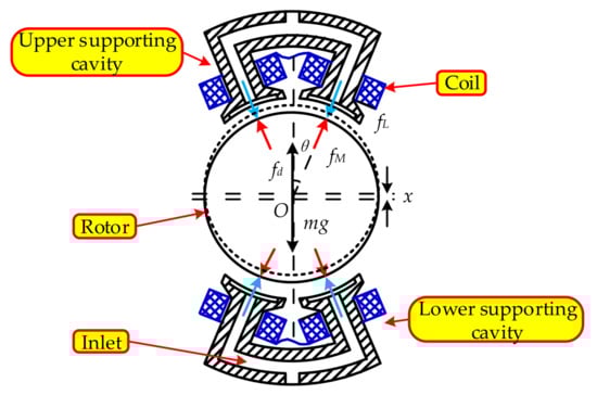
Figure 6.
Structure diagram of the single-DOF system.
According to the Maxwell attraction formula, the electromagnetic force can be obtained as follows [10].
where, fM,1 is electromagnetic force of upper pole, the unit is N. fM,2 is electromagnetic force of lower pole, the unit is N. k is current constant, the unit is H·m, and . μ0 is air permeability, the unit is H/m. N is turns of coil, the unit is dimensionless. As is magnetic’s area, the unit is m2. i0 is bias current, the unit is A. h0 is thickness of oil film, the unit is m. l is thickness of coating, the unit is m. x is displacement of rotor, the unit is m. θ is angle, the unit is °.
According to the Navier-Stokes equation, the hydrostatic supporting force can be obtained as follows [11].
where, fL,1 is hydrostatic force of upper supporting cavity, the unit is N. fL,2 is hydrostatic force of lower supporting cavity, the unit is N. k1 is stiffness factor, the unit is L/min/V. u0 is flow of lower supporting cavity, the unit is m3/s. Ab is extrusion area, the unit is m2. Rh,1 is liquid resistance of upper supporting cavity, the unit is kg/(m4·s), and . Rh,2 is liquid resistance of lower supporting cavity, the unit is kg/(m4·s), and . μ is viscosity, the unit is Pa·s. is flow coefficient, the unit is dimensionless. Ae is supporting area, the unit is m2.
The Taylor expansion of resultant force on the rotor at x = 0, , i0 = 0, u0 = 0 is shown as follows.
where, kx is displacement stiffness coefficient, the unit is dimensionless. kv is velocity stiffness coefficient, the unit is dimensionless. ku is voltage stiffness coefficient, the unit is dimensionless. ki is current stiffness coefficient, the unit is dimensionless.
3. Mathematical Model of the Multi-DOF Supporting System
3.1. Dynamic Equation of the Multi-DOF Supporting System
In order to study the supporting characteristics of the multi-DOF system, the following assumptions are made [12,13,14,15]:
- (1)
- The flow condition of the lubrication is laminar and the inertia force is ignored.
- (2)
- The viscosity-pressure characteristics of the lubrication are ignored due to the low pressure.
- (3)
- The winding magnetic flux leakage is ignored and the flux is evenly distributed in the magnetic circuit.
- (4)
- The magnetoresistance in the iron core and rotor is ignored, and the magnetic potential only acts on the air gap.
- (5)
- The hysteresis and eddy of magnetic materials are ignored.
- (6)
- The supporting surface is assumed to be a rigid body.
- (7)
- The gravity of the rotor is ignored.
- (8)
- The rigid rotor is geometrically symmetrical uniform, Jx = Jy = Jr.
- (9)
- The rotor is in the rotation center, the bearing force is zero, and there is no interference between the DOF supporting system.
- (10)
- The installation error of the sensor is not considered.
- (11)
- The stiffness of the base is relatively large, and there is no deformation or movement.
The rotor’s force model of the MLDSB is established as shown in Figure 7.
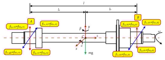
Figure 7.
Force diagram of the rotor.
The fixed coordinate system Cxyz is established, and the origin is the mass center of the rotor. According to Figure 7, the expression of the mechanical relationship is assumed as follows.
where, the meanings of subscripts x, y, L, M, A, and B are x direction, y direction, hydrostatic force, electromagnetic force, bearing A, and bearing B respectively.
The displacement on the sensors at the left and right ends is converted to the mass center C, and the displacement xc and yc are approximately shown as follows.
where, l is length of the rotor, the unit is mm. la, lb is distance of center and left-unit, distance of center and right-unit respectively, the unit is mm. xc, yc is displacement of the mass center, the unit is mm. xA, yA is displacement of the right unit, the unit is mm. xB, yB is displacement of the left unit, the unit is mm.
where, θx is angle at plane yz, the unit is °. θy is angle at plane xz, the unit is °.
The torque of the rotor is shown as follows.
where, Jr is inertia moment of the rotor around the x and y-axis, the unit is kg·m2. Ja is inertia moment of the rotor around the z-axis, the unit is kg·m2.
According to Equations (1)–(7), the force equation of the rotor can be obtained as follows.
3.2. Selection of Design Parameters
The design parameters of the MLDSB are shown in Table 1.

Table 1.
Design parameters of the MLDSB.
3.3. Coupling Relationship Analysis
When the rotor is in the rotation center, the initial gap is δ0. According to the geometric relation, the gap at any time is shown as follows.
where, is initial gap, the unit is m. is gap of bearing A in x-direction, the unit is m. is gap of bearing B in x-direction, the unit is m. is gap of bearing A in y-direction, the unit is m. is gap of bearing B in y-direction, the unit is m.
So
According to Equations (7)–(10), there is interference between the x and y direction of the left unit and right unit. In other words, there is a coupling effect between the spatial positions and postures which can affect the operation stability of the MLDSB. There is no coupling between the axial direction and radial direction. Additionally, there is a space position coupling between the radial direction and rotation direction.
4. Decoupling Control of the Multi-DOF System
4.1. Design of the Decoupling Device
The electromagnetic force and hydrostatic force of each supporting system are controlled by the dual input differential method, and the inputs can be combined as shown in Equation (11).
where Ii is the input current, Ui is the input voltage.
The state variable can be selected as follows.
The output variable can be selected as follows.
According to Equations (1)–(10), the state space equation can be obtained as follows.
The state feedback decoupling strategy is a decoupling method that combines the state feedback control law with the α inverse decoupling theory. Namely, the control law is shown as follows.
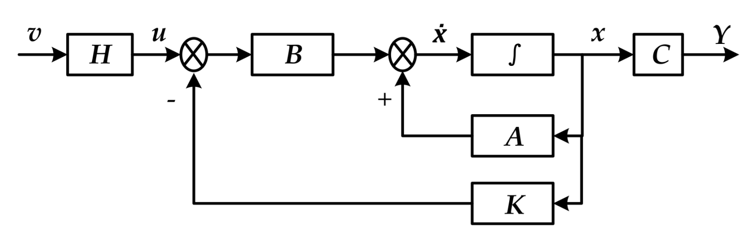
The specific structure is shown in Figure 8.

Figure 8.
Block diagram of state feedback decoupling method.
The state-space expression after construction is shown as follows.
where x is n × 1 state vector, u is l × 1 input vector, y is m × 1 output vector, A is n × n state matrix, B is n × l input matrix, C is m × n output matrix.
In the α-order inverse decoupling theory, the desired closed-loop matrix GL(s) is set to the diagonal form, so that the output matrix Y is the α-order integral of the input matrix X with respect to time as shown in Equations (17) and (18).
According to Equation (14), the target of multi-DOF decoupling is to transform G(s) into the decoupled diagonal matrix form by selecting the feedback matrix K and feedforward matrix H based on the α-order inverse decoupling theory.
In the α-order inverse decoupling theory, non-singular matrices E and F are defined to solve K and H, and its expressions are defined as follows.
where, α = (αi) is the decoupling order constant. The solution idea of α is as follows.
- (1)
- For G(s), the output equation can be seen from the state-space equation as follows.where Y contains i output components and C contains the i row vectors.
- (2)
- Take the derivative of both ends of the above equation with respect to time t, and substitute the state equation into Equation (21).
If ciB ≠ 0, set αi = 1, the following equation will be found:
Similarly, if ciAB ≠ 0, set αi = 2, continue to derivative until ciAαi−1B ≠ 0. Arrange Equation (23), and the decoupling order constant can be defined as follows.
Respectively replace A, B, and C with Az, Bz, and Cz, and get αi = 2. Combining Equations (18) and (19), it can be shown as follows.
Thus, the following equation can be obtained.
Combined with Equation (19), the control law coefficient relation can be obtained as follows.
Because E is a nonsingular matrix, and its inverse is also a nonsingular matrix, therefore, the 2nd and 3rd of the time domain decoupling constraints are proven. With the above proof, it can be obtained that the system can be decoupled in the time domain, and the transformation matrix and state feedback control law matrix are brought in and the decoupling effect is as follows.
4.2. Design of the Controller
The fundamental idea of the system controller is to make the closed-loop pole of the system at the desired point by adjusting the open-loop zero pole of the system to achieve the performance indexes related to the system [16].
The main principle of applying the root locus method to the system correction is that the closed-loop leading poles of the system are first set so that the closed-loop dynamic performance of the system can be approximated by the second-order system with closed-loop leading poles [17,18].
Therefore, before the introduction of a lead corrector, the time domain performance index of the system must be transformed into an equation with leading poles. After the introduction of a lead corrector, the calibrated system is made to work at the desired dominant pole, while other poles of the system exist away from the imaginary axis of the s-plane or close to a certain zero of the system [19,20,21].
It is assumed that the expected time-domain index for the MLDSB is as follows.
According to Equation (29), the expected dominant pole sd after correction can be obtained as follows:
Establish the mathematical model of the lead correction link.
According to the root trajectory diagram method, the zero poles of the lead correction link respectively are Zc = 2273, Pc = 1.1 × 10⁴. According to the system gain calculation method, the system gain is K = 5.5 × 10⁷. The corrected root locus is shown in Figure 9.
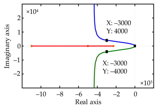
Figure 9.
Root locus after correction.
The root locus passes through the closed-loop leading pole sd, and is able to meet system requirements.
5. MATLAB\Simulink Simulation
Based on the Simulink development platform, the MLDSB is taken as the controlled object, and the block diagram using the state feedback approach is shown in Figure 9. The matrix-vector modem is adapted in gains, and the solution methods of matrix A, B, C, K, and H are shown in Equations (11)–(27). To observe the decoupling effect, the double differential module is added after decoupling [22,23].
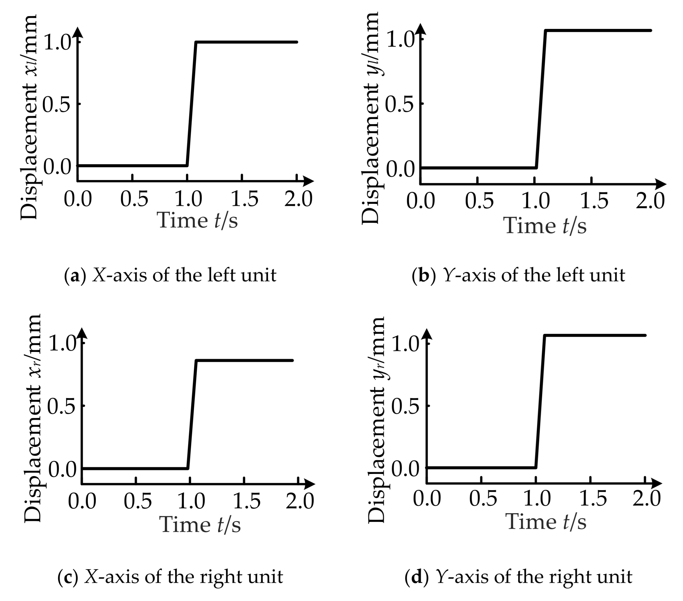
According to Figure 10, taking the step signal as an example at the initial stage (V = 1 A, t = 1 s), the simulation curves are shown in Figure 11.
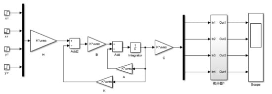
Figure 10.
Simulink block diagram.

Figure 11.
Displacement of the rotor under a step signal.
According to Equation (28), the diagonal element of the output is 1/s2, and its output matrix is a negative identity matrix after two differentials. According to Figure 10, it can be observed that each channel of the system is given at 1 s, after the step signal was given, each position was adjusted to 1 mm after about 0.08 s.
After comparison, the results were consistent with the theoretical calculation results.
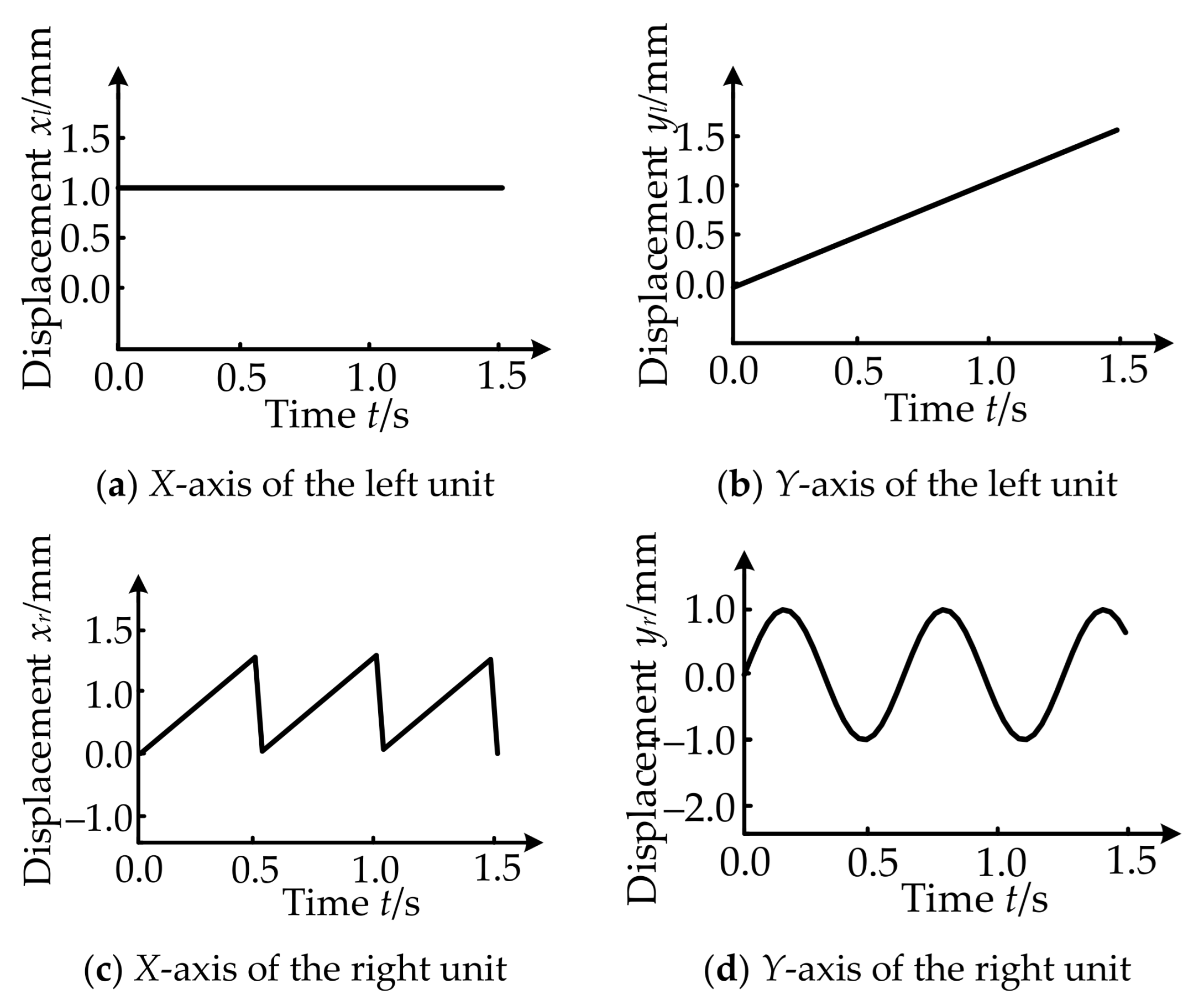
The decoupling simulation of the system requires that the system has the ability to distinguish between output signals when the input terminal gives different signals, so it is necessary to determine the decoupling effect by different waveforms given at the input terminal of the different channels in the system. The signal input is shown in Figure 12.
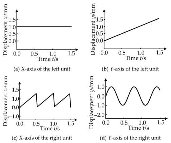
Figure 12.
Input signal.
The output response of the decoupled system is shown in Figure 13.

Figure 13.
Displacement of the rotor under the input signal.
It can be seen from Figure 13 that after different input signals are input into different channels, the corresponding channels can produce relative output changes which have a slight influence on the remaining channels. In other words, the decoupling between the displacement changes and the input signals of the multi-DOF system of the MLDSB can be achieved.
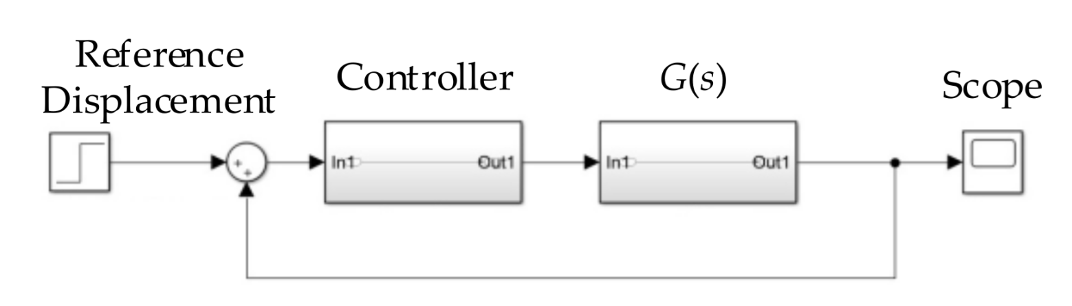
The block diagram after adding displacement feedback is shown in Figure 14.
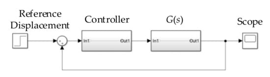
Figure 14.
Control block diagram.
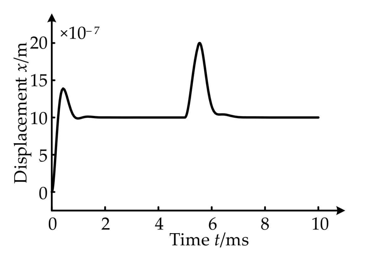
By setting the reference displacement to 10 μm and external interference to 200 N, the above block diagram is simulated. The output response curve of the displacement of the single-DOF system is shown in Figure 15.

Figure 15.
Output response curve of the rotor.
According to Figure 14, the system tends to stabilize at the desired displacement of 10 μm at 0.1 ms after loading. With a load interference force of 200 N after 5 ms, the rotor of the system changes by 10 μm, which is much less than the gap of 30 μm. When the external disturbance disappeared, the output response of the rotor displacement is reduced to the expected value. The change conforms to the expected conditional value.
6. Experimental Result of Decoupling
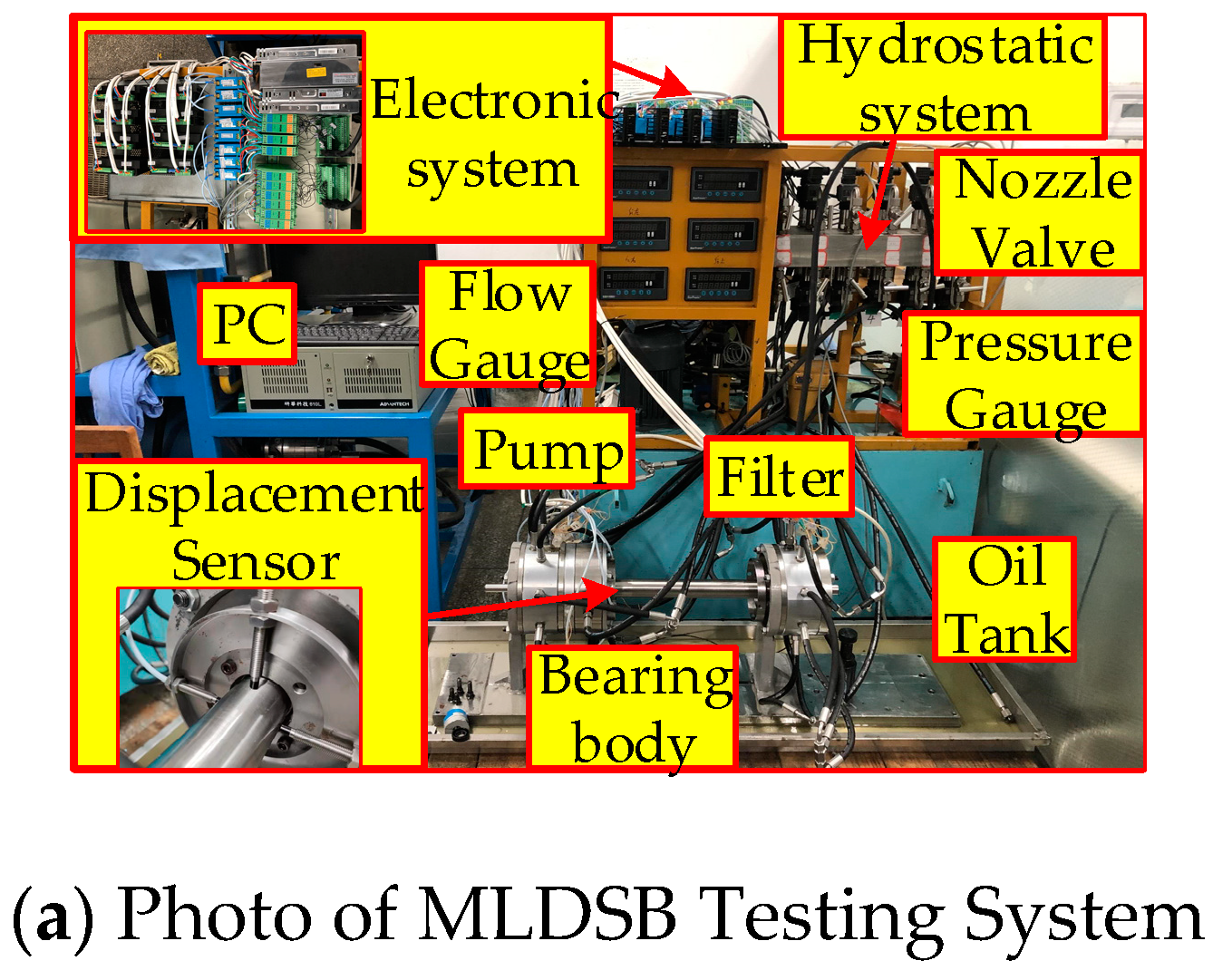
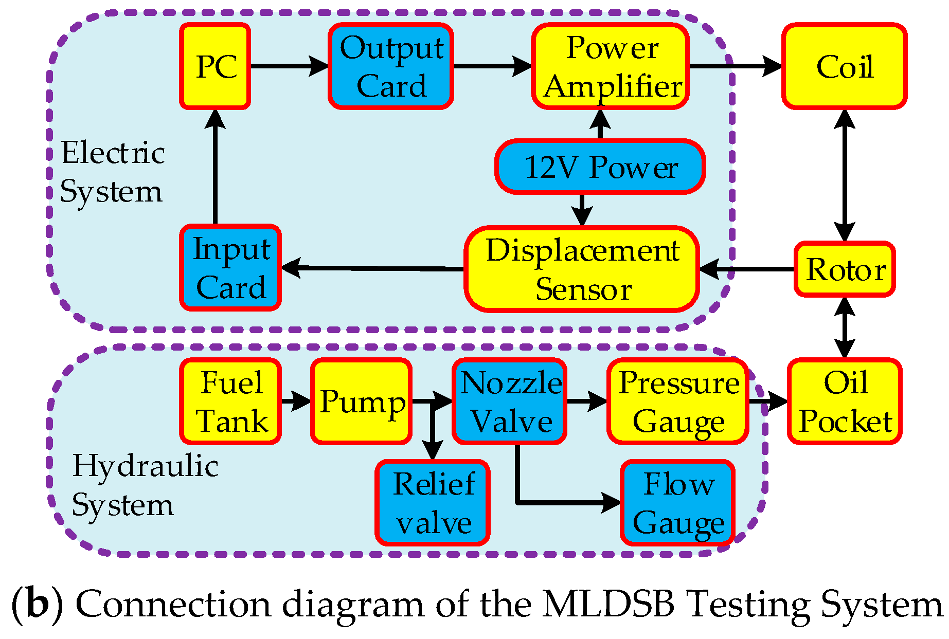
6.1. Brief Introduction of the MLDSB Testing System
The MLDSB Testing System is composed of the electronic control system, hydrostatic system, and bearing body as shown in Figure 16.
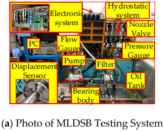
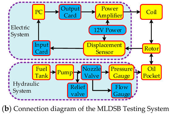
Figure 16.
MLDSB Testing System.
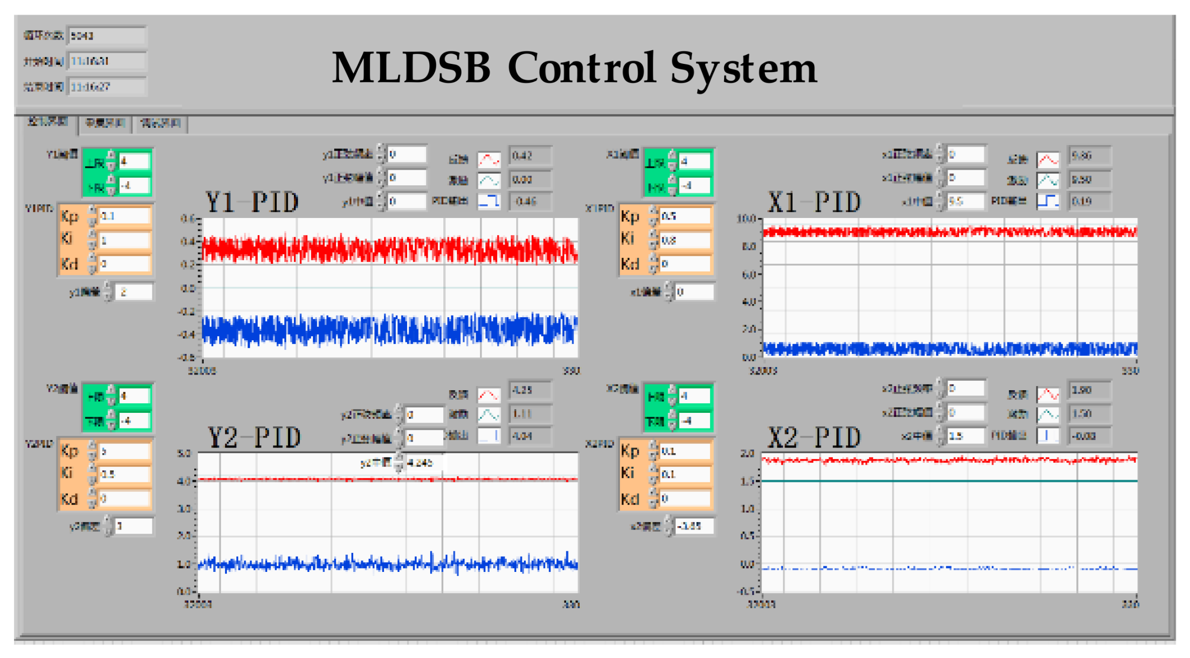
The MLDSB Testing System uses LabVIEW software to process the acquired signals, and the PC Collecting Interface is shown in Figure 17.
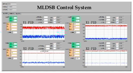
Figure 17.
PC Collecting Interface of the MLDSB Testing System.
The hydrostatic system is a constant pressure supporting model, and its flow is adjusted by a needle valve. The electronic control system is a closed-loop position control system, and its current is adjusted by a PID controller.
The component’s parameters of the MLDSB Testing System are shown as follows.
- (1)
- Hydraulic pump, model TGPVL4-200SH, manufacturers for Taixing Hongsheng Hydraulic Co., Ltd., Taixing, China. Pressure 14 MPa, flow 16 L/min, rotation speed 1450 r/min.
- (2)
- Relief valve, model DBD-H-6-P-10-B-NG10, manufacturers for Beijing Huade Hydraulic Industrial Group Co., Ltd., Beijing, China. Pressure 10 MPa, size 6 mm.
- (3)
- Nozzle valve, model A7-2-KL2-0KL20-PTFE, manufacturers for Shanghai Hawk Fluid Control Co. Ltd., Shanghai, China. Size 6 mm.
- (4)
- Flow gauge, model LWGY-S, manufacturers for Nanjing Detair Instrument & Electromechanical Equipment Co. Ltd., Nanjing, China. Pressure 2 MPa, flow 120–2400 mL/min, accuracy 2%.
- (5)
- Pressure gauge, model HSTL-802, manufacturers for Beijing Huakong Xingye Technology Development Co., Ltd., Beijing, China. Pressure 10 MPa, accuracy 0.25%.
- (6)
- Displacement gauge, model VB-Z9900, manufacturers for Shanghai Ann Electronic Technology Co., Ltd., Shanghai, China. Range of 4 mm, accuracy 1.5%.
- (7)
- Coil, manufacturers for Sanhan Tin Co., Ltd., Kunshan, China. Materials for Cu, diameter 1.0 mm, electrical resistivity 0.02240 Ω/m, length 25 m.
- (8)
- PC, model IPC-610L, manufacturers for Taiwan Advantech Co., Ltd., Taiwan, China. Mainboard AIMB-705BG, CPU I5-6500.
- (9)
- Output card, model NI6723, manufacturers for America NI instruments Co., Ltd., Texas, America. 8 channels output.
- (10)
- Input card, model PCI1716, manufacturers for Taiwan Advantech Co., Ltd., Taiwan, China. 16 channels input,
- (11)
- 12V Power, model S1500-12, manufacturers for China Meanwell Group Co., Ltd., Guangzhou, China. Voltage 12V, current 125 A, power 1500 W.
- (12)
- Power amplifier, model AQMD3620NS-A2, manufacturers for Chengdu Aikong Electric Technology Co. Ltd., Chengdu, China. Power 400 w, input voltage 36 V, current 16 A.
6.2. Experimental Procedure
The experimental procedure of static bifurcation is shown as follows.
- (1)
- Switch on the power, set the PID parameter in the y-direction to 0, adjust Kp and Kd in the x-direction, and make the rotor oscillate in constant amplitude.
- (2)
- Adjust i0 to make the rotor stably suspended in the initial position in the x-direction, and record the Kp, Kd, and i0.
- (3)
- Similarly, Set the PID parameter in the x-direction to 0, adjust Kp and Kd parameters in the y-direction, and make the rotor oscillate in constant amplitude.
- (4)
- Similarly, adjust i0 to make the rotor stably suspended in the initial position in the y-direction, and record the Kp, Kd, and i0.
- (5)
- Re-input Kp, Kd, and i0 in the x and y directions, and collect the displacement-time curve.
- (6)
- Add the decoupling controller to the LabVIEW program, repeat step 1~step 5, adjust the controller compensation coefficient to make the rotor operate stably, and collect the displacement-time curve.
6.3. Analysis of Experimental Results
According to Figure 6 and Figure 7, the magnetic circuit coupling between each magnetic pole of the stator can reduce the control accuracy of the channel and the stable suspension of the MLDSB.
- (1)
- Magnetic circuit coupling characteristics between channel x and channel y.
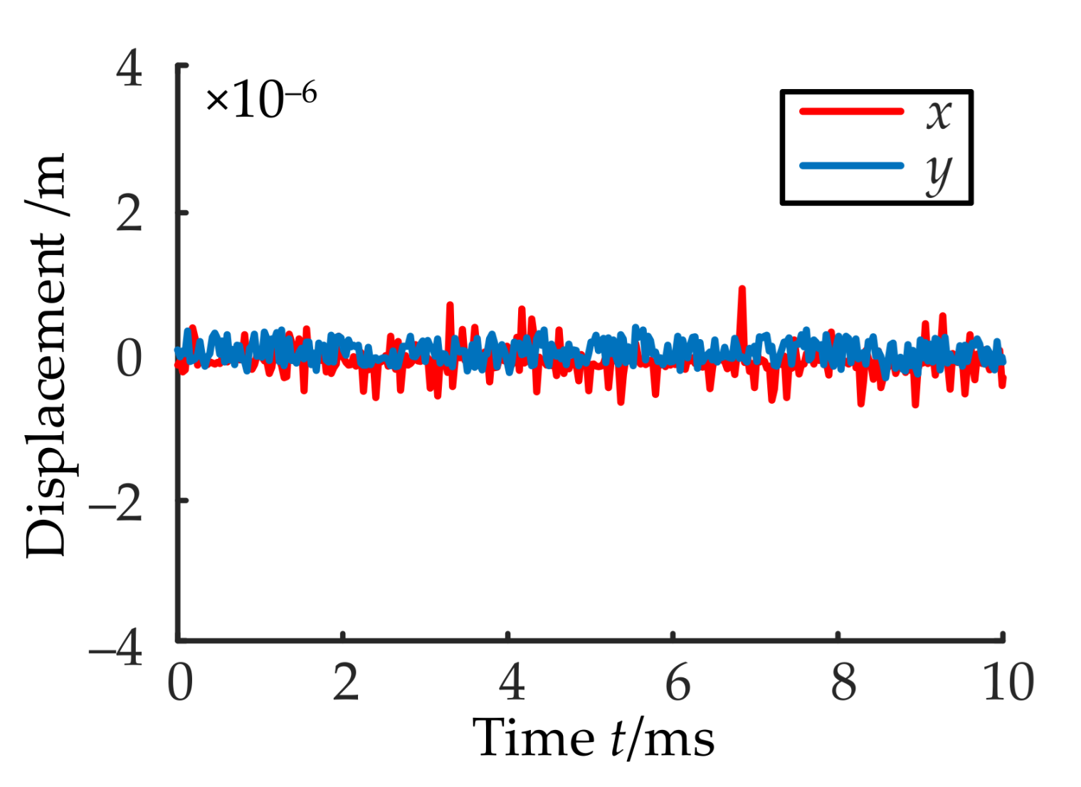
In order to explore the magnetic circuit coupling characteristics between channel x and channel y of the stator, only channel x or channel y is opened to achieve single-channel electromagnetic suspension. The steady-state displacement of the rotor is tested as shown in Figure 18.

Figure 18.
Steady-state displacement under single suspension.
According to Figure 16, the rotor can be stably suspended by channel x/y, the displacement is within the range of (−1, 1) μm, and the requirements of engineering practice can be met.
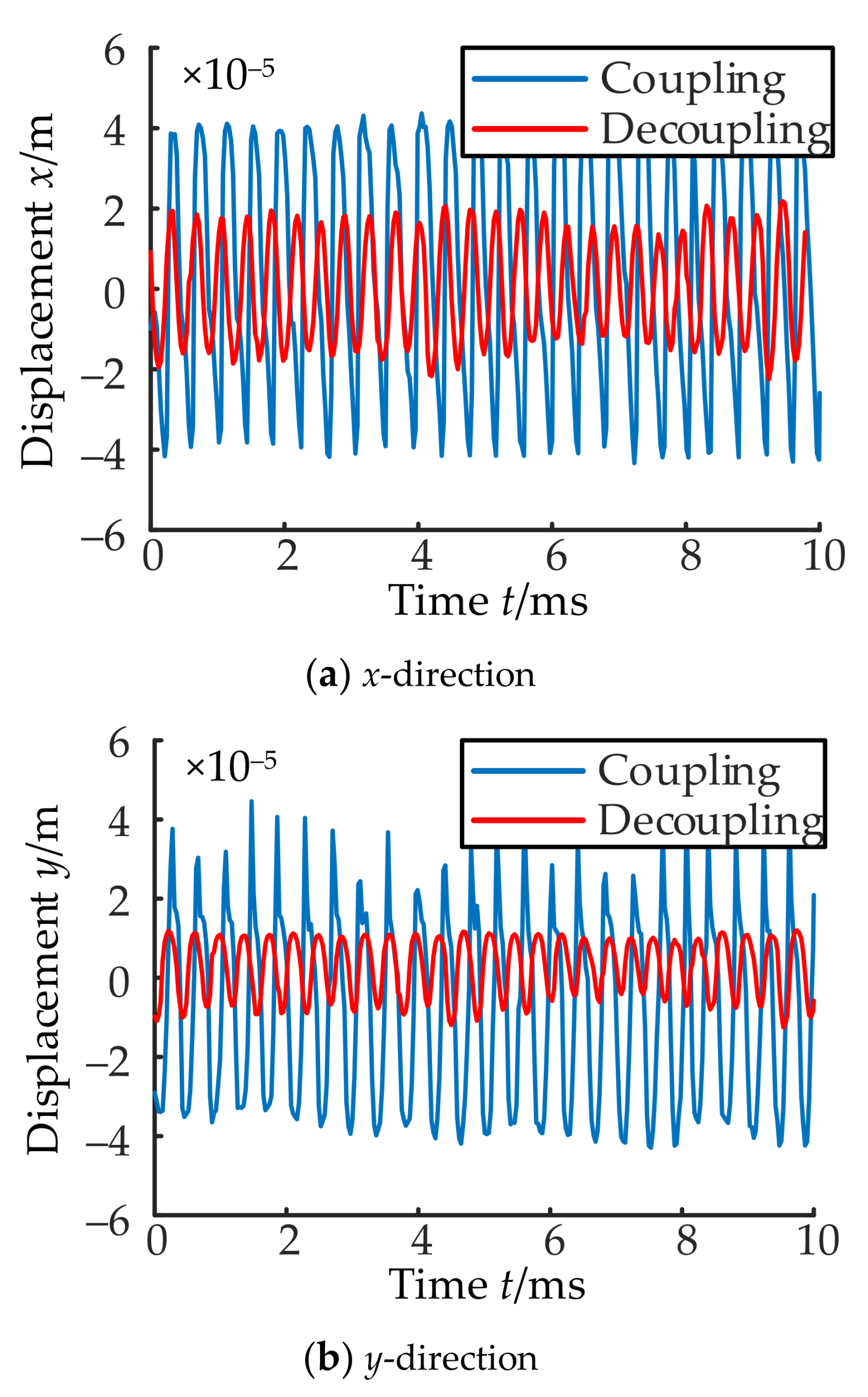
When channel x and channel y are opened, the steady-state displacement is obtained by the test as shown in the blue curve in Figure 19 and Figure 20.
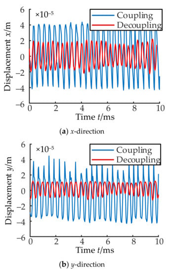
Figure 19.
Displacement of the rotor without rotation.
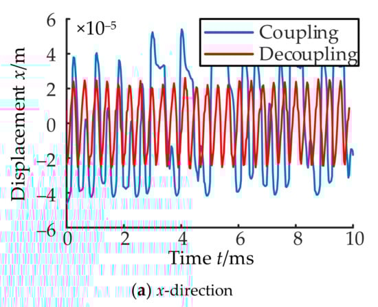
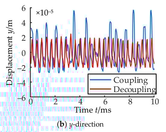
Figure 20.
Displacement of the rotor with rotation.
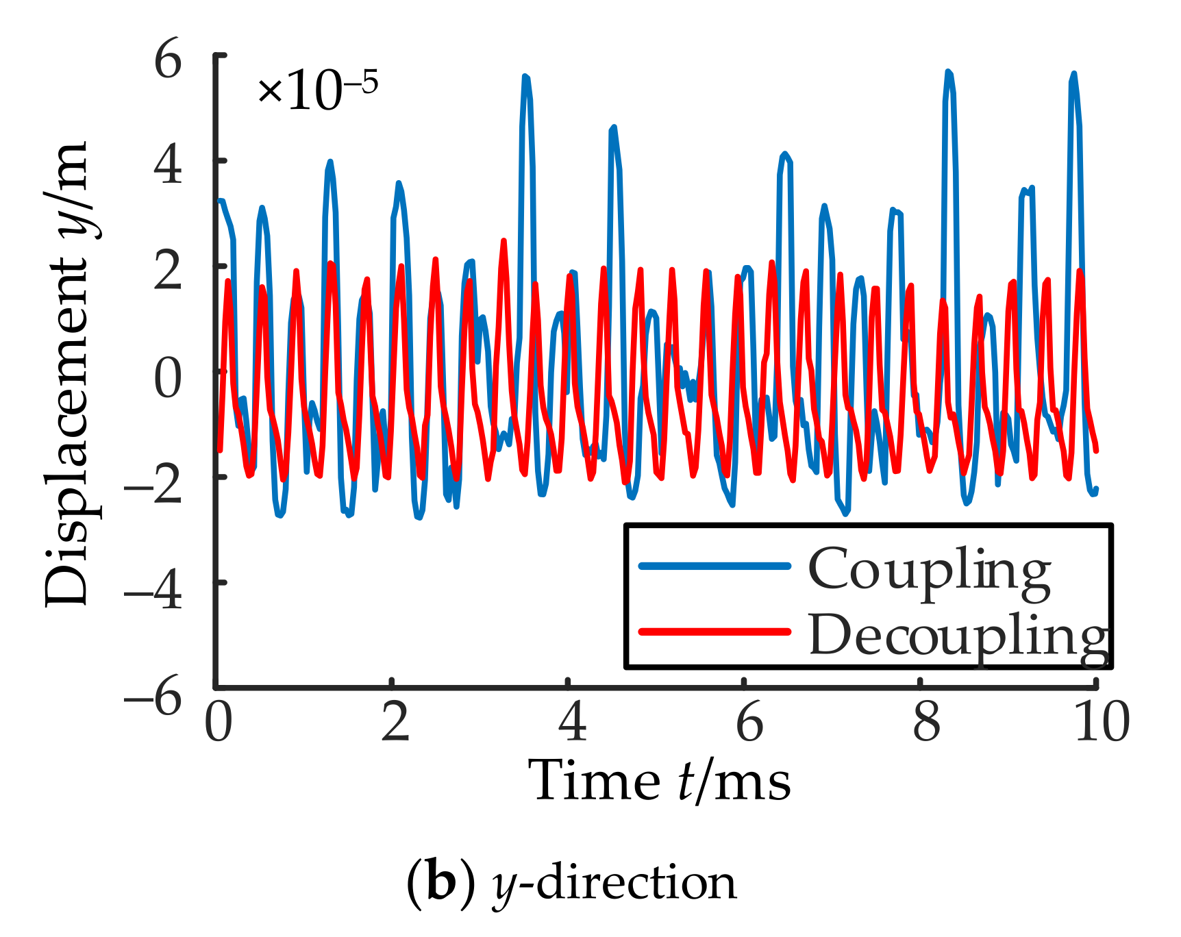
According to Figure 19 and Figure 20, the rotor moves irregularly, and its displacement increases greatly. It is basically limited within the range of (−40~40) μm and reached the design value of oil film thickness, and then, the rotor cannot be suspended stably. The coupling phenomenon in the rotation state is more obvious than with no rotation, and the peak fluctuation phenomenon of the steady-state displacement appears at the same frequency.
By comparing Figure 18, Figure 19 and Figure 20, it can be seen that the magnetic circuit coupling between the magnetic poles is large, and the control accuracy and stability of channel x and channel y is greatly reduced.
- (2)
- Magnetic circuit decoupling between channel x and channel y.
Based on the coupling characteristics of the magnetic circuit and the above decoupling theory, channel x and channel y are decoupled and controlled to obtain the decoupling displacement of the rotor as shown in the red curve of Figure 19 and Figure 20.
According to Figure 19 and Figure 20, the rotor returns to the equilibrium position after decoupling, and it vibrates regularly in the y-direction and x-direction. There is minimal interference between the y-direction and x-direction. Compared to before the decoupling, the steady-state displacement is significantly reduced from (−40~40) μm to (−20~20) μm, and the decoupling effect of channel y is greatly improved.
- (3)
- Regulation characteristics of channel x and channel y after decoupling.
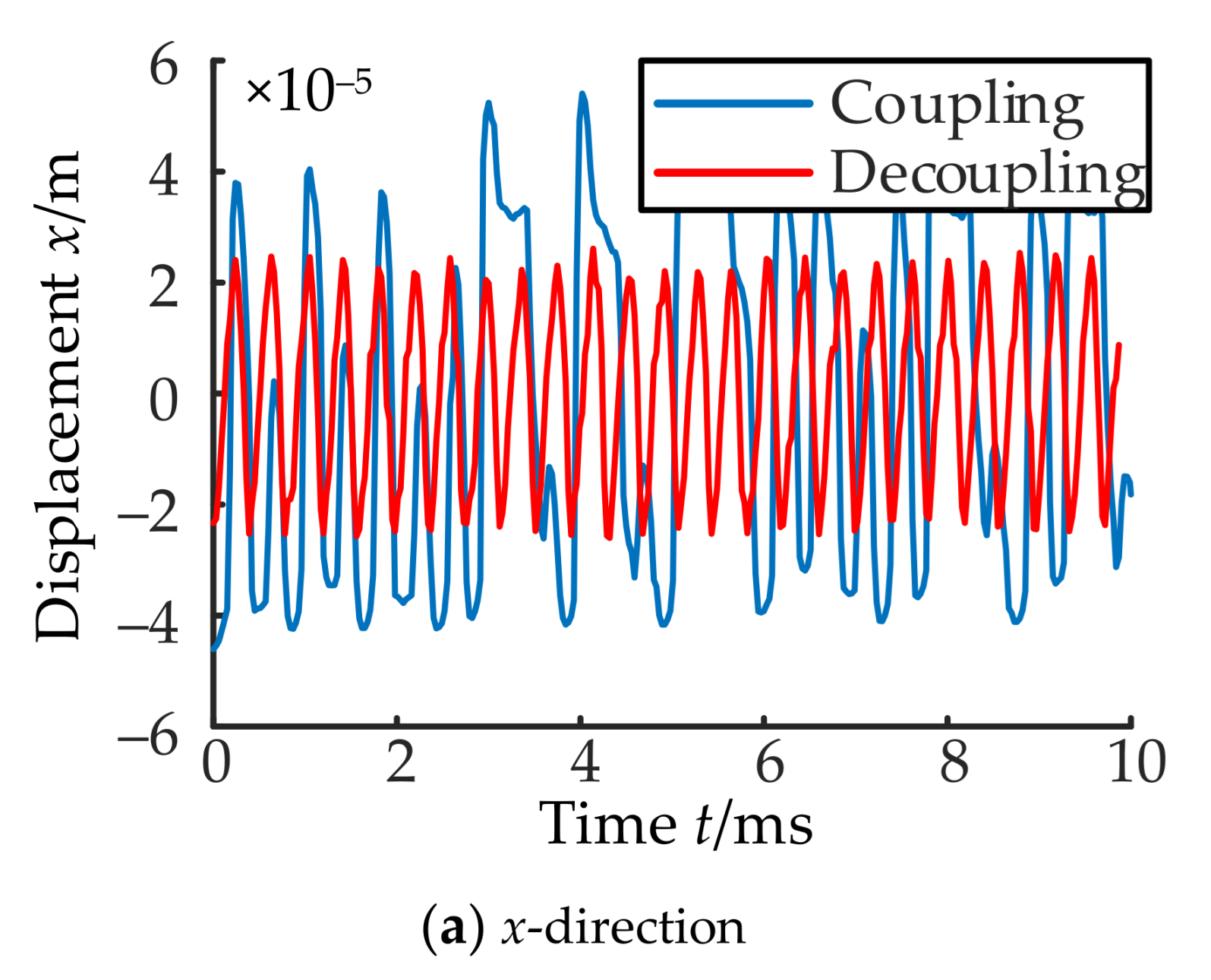
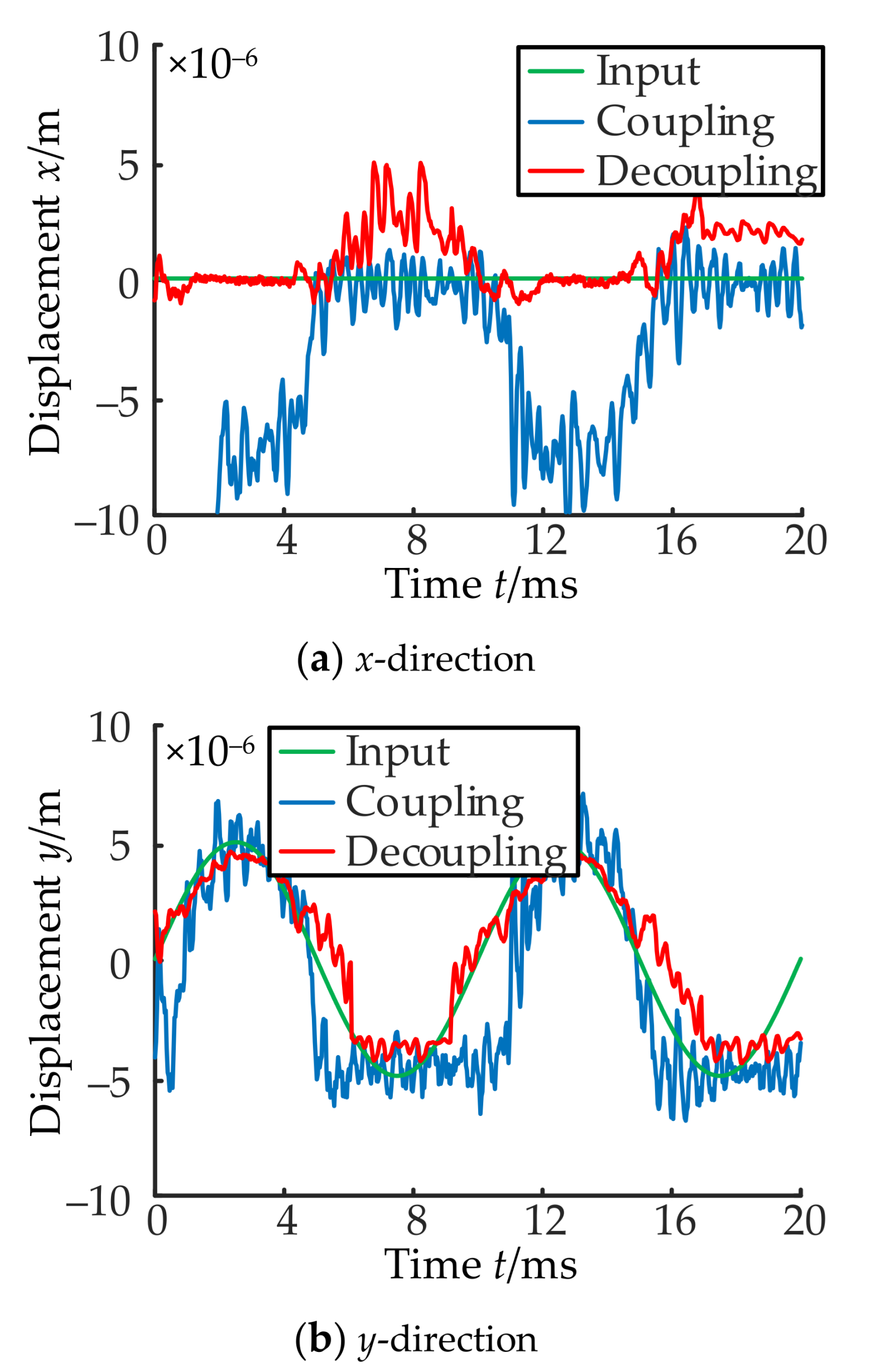
In order to further study the regulation characteristics of each channel after decoupling, the sinusoidal signal (amplitude is 5 μm and period is 10 ms) is given in the x-direction and y-direction respectively, and the following curves are obtained as shown in Figure 21 and Figure 22.
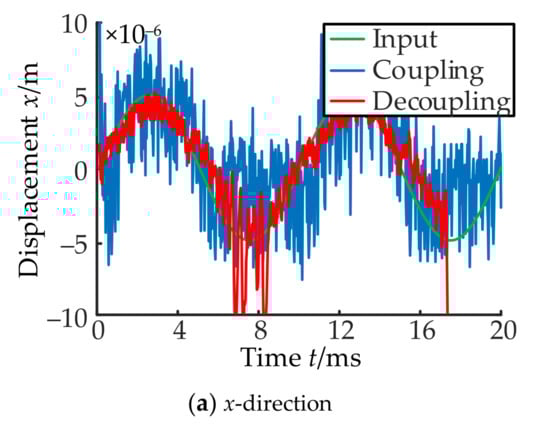

Figure 21.
Displacement under sinusoidal signal in channel x.
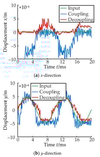
Figure 22.
Displacement under sinusoidal signal in channel y.
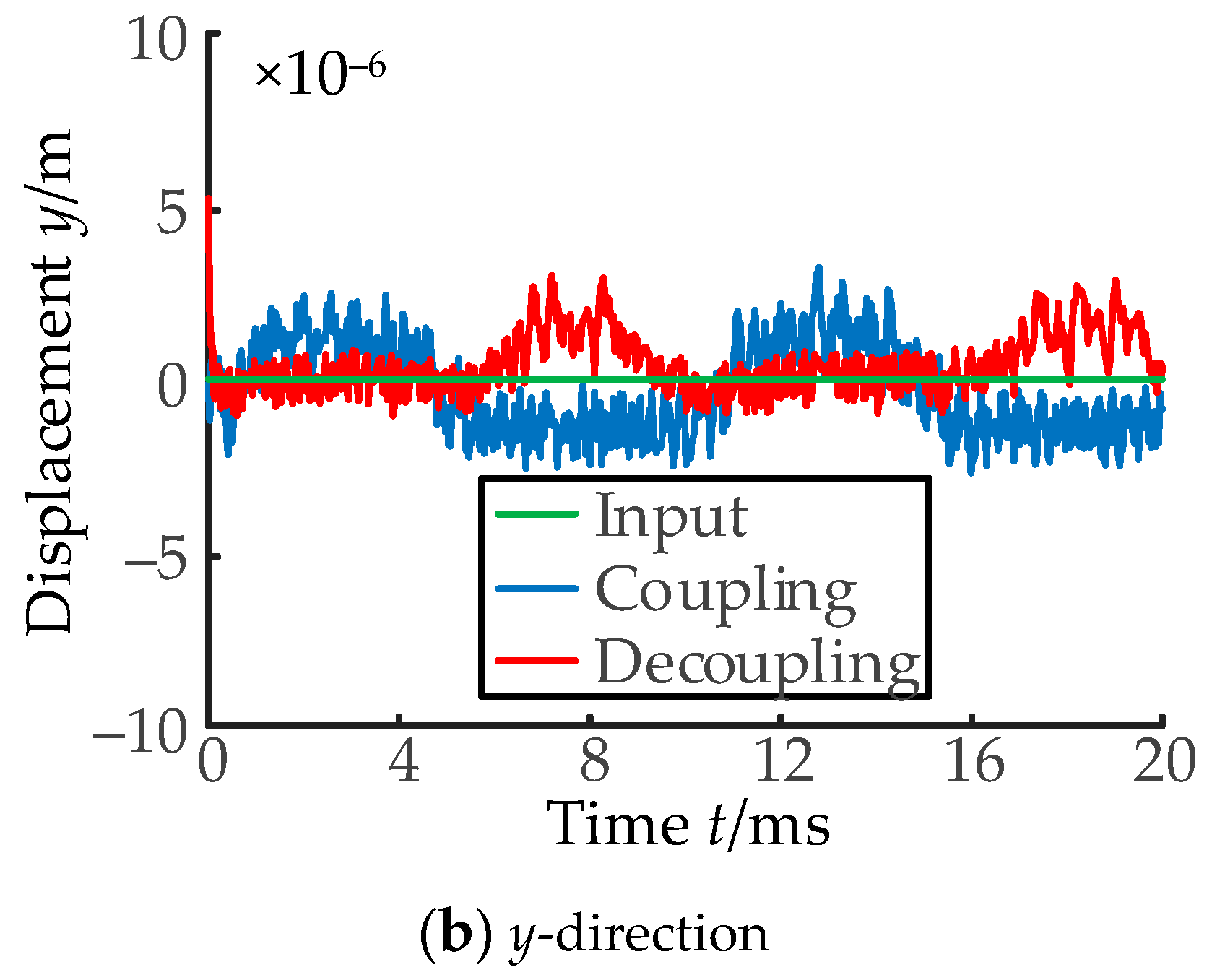
According to Figure 21 and Figure 22, the rotor displacement before decoupling in the input channel presents the sinusoidal motion law with high-frequency oscillation as shown in the blue curve of Figure 21a and Figure 22b. After decoupling, the decoupling controller effectively eliminates the oscillation and greatly improves the displacement with the characteristics as shown in the red curve of Figure 21a and Figure 22b.
Due to the coupling characteristics of the magnetic circuit, the rotor displacement before decoupling in the non-input channel is also affected by the coupling of the input channel, and it shows a small sinusoidal motion with the same frequency as shown in the blue curve of Figure 21b and Figure 22a.
After decoupling, the decoupling controller effectively eliminated the rotor high-frequency oscillation and greatly improved the zero-retaining characteristic of rotor displacement, and then the decoupling effect of channel y is greatly improved as shown in the red curve of Figure 21b and Figure 22a. The theoretical correctness of the decoupling controller can be effectively proven.
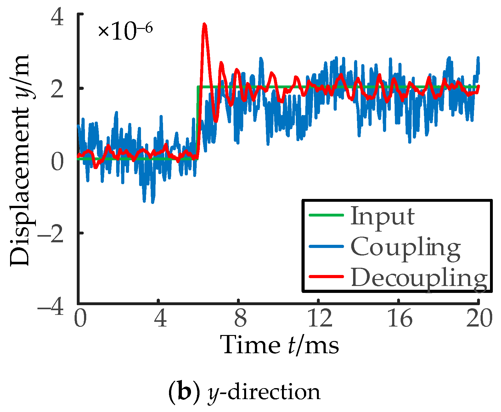
Similarly, the step signal (Amplitude is 2 μm and time is 6 ms) is given in the x-direction and y-direction respectively, and the subsequent displacement curves before and after decoupling are obtained as shown in Figure 23 and Figure 24.
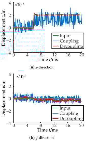
Figure 23.
Displacement under step signal in channel x.
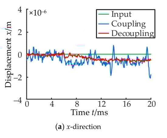

Figure 24.
Displacement under step signal in channel y.
According to Figure 23 and Figure 24, the rotor displacement before decoupling in the input channel present the step motion law with high-frequency oscillation as shown in the blue curve of Figure 23a and Figure 24b. After decoupling, the decoupling controller effectively eliminates high-frequency oscillation of the rotor and greatly improves the displacement characteristics as shown in the red curve in Figure 23a and Figure 24b.
Due to the coupling characteristics of the magnetic circuit, the rotor displacement before decoupling in the non-input channel is also affected by the coupling of the input channel, and it shows a small motion with the same frequency as shown in the blue curve of Figure 23b and Figure 24a. After decoupling, the decoupling controller effectively eliminates the rotor high-frequency oscillation and greatly improves the zero-retaining characteristic of the displacement as shown in the red curve of Figure 23b and Figure 24a. Then, the theoretical correctness of the decoupling controller can be effectively proven.
7. Conclusions
- (1)
- In this paper, the state feedback decoupling method is used to realize the decoupling control of the multi-DOF MLDSB supporting system. The multi-DOF system is effectively separated into the single-DOF system.
- (2)
- The lead corrector determined by the root locus method can improve the dynamic characteristics and anti-jamming ability of the decoupling system.
- (3)
- Coupling characteristics between channel x and channel y and the decoupling effect of the controller are tested experimentally. The results show that the coupling effect is reduced by use of the decoupling controller, the subsequent displacement characteristics of the rotor and the operational stability of the MLDSB can be improved greatly.
Author Contributions
Conceptualization, F.H. and G.Z.; methodology, F.H. and G.Z.; software, F.H. and G.Z.; validation, F.H., Y.W. and X.Z.; formal analysis, Y.W.; investigation, G.Z.; resources, J.Z.; data curation, F.H. and Y.W.; writing—original draft preparation, F.H. and G.Z.; writing—review and editing, F.H.; visualization, J.Z.; supervision, J.Z.; project administration, J.Z. and G.D.; funding acquisition, J.Z. All authors have read and agreed to the published version of the manuscript.
Funding
This research was funded by the National Nature Science Foundation of China, grant number 52075468 and number 52005428; General project of Natural Science Foundation of Hebei Province, grant number E2020203052 and number 2021203099); Youth Fund Project of a scientific research project of Hebei University, grant number QN202013.
Institutional Review Board Statement
Not applicable.
Informed Consent Statement
Not applicable.
Data Availability Statement
No new data were created or analyzed in this study. Data sharing is not applicable to this article.
Conflicts of Interest
The authors declare no conflict of interest.
References
- Belila, A.; El-Chakhtoura, J.; Otaibi, N.; Muyzer, G.; Gonzalez-Gil, G.; Saikaly, P.E.; van Loosdrecht, M.C.; Vrouwenvelder, J.S. Bacterial Community Structure and Variation in a Full Scale Seawater Desalination Plant for Drinking Water Production. Water Res. 2016, 94, 62–72. [Google Scholar] [CrossRef] [PubMed] [Green Version]
- Dong, G.; Kim, J.F.; Kim, J.H.; Drioli, E.; Lee, Y.M. Open-Source Predictive Simulators for Scale-Up of Direct Contact Membrane Distillation Modules for Seawater Desalination. Desalination 2017, 402, 72–87. [Google Scholar] [CrossRef]
- Zhao, J.H.; Chen, T.; Wang, Q.; Zhang, B.; Gao, D.R. Stability Analysis of Single DOF Support System of Magnetic-Liquid Double Suspension Bearing. Mach. Tool Hydraul. 2019, 47, 1–7. [Google Scholar]
- Wang, Y.Z.; Jiang, D.; Yin, Z.W.; GAO, G.Y.; ZHANG, X.L. Load Capacity Analysis of Water Lubricated Hydrostatic Thrust Bearing Based on CFD. J. Donghua Univ. 2015, 41, 428–432. [Google Scholar]
- Ming, Z.; Tong, W.; Dapeng, W. Feed-Forward Compensation Decoupling Control for Hybrid Radial Magnetic Bearing used in High Speed Electric Machine. Trans. China Electrotech. Soc. 2015, 30, 539–544. [Google Scholar]
- Zhao, H.Y.; Zhu, C.S. Feedforward Decoupling Control for Magnetically Suspended Rigid Rotor System. J. Zhejiang Univ. 2018, 52, 152–162. [Google Scholar]
- Chen, L.; Zhu, C.; Wang, Z. Two-Degree-of-Freedom Control for Active Magnetic Bearing Flywheel Rotor System Based on Inverse System Decoupling. Trans. China Electrotech. Soc. 2017, 32, 100–114. [Google Scholar]
- Si, M. Research on Current Loop Deviation Decoupling Control Strategy of Permanent Magnet Synchronous Motor. Master’s Thesis, Xi’an University of Technology, Xi’an, China, 2019. [Google Scholar]
- Zhao, J.H.; Chen, T.; Han, F.; Gao, D.R.; Du, G.J. Research on robust control strategy of single DOF supporting system of MLDSB based on H∞ mixed-sensitivity Method. High Technol. Commun. 2020, 26, 299–305. [Google Scholar]
- Zhang, W.; Cheng, L.; Zhu, H. Suspension force error source analysis and multidimensional dynamic model for a centripetal force type-magnetic bearing. IEEE. Trans. Ind. Electron. 2020, 67, 7617–7628. [Google Scholar] [CrossRef]
- Wang, N.; Jiang, D.; Behdinan, K. Vibration response analysis of rubbing faults on a dual-rotor bearing system. Arch. Appl. Mech. 2017, 87, 1891–1907. [Google Scholar] [CrossRef]
- Zhao, J.H.; Zhang, G.J.; Cao, J.B.; Gao, D.R.; Du, G.J. Decouping Control of Single DOF Supporting System of Magnetic-Liquid Double Suspension Bearing. Mach. Tool Hydraul. 2020, 48, 1–8. [Google Scholar]
- Jin, W.H.; Jin, S.; Jiang, W. Torque Decoupled Vector Control of Permanent Magnet Reluctance Hybrid Rotor Dual-stator Synchronous Motor. Large Electr. Mach. Hydraul. Turbine 2021, 1, 20–23. [Google Scholar]
- Reza, E.; Mostafa, G.; Mohammad, K.H. Nonlinear Dynamic Analysis and Experimental Verification of a Magnetically Supported Flexible Rotor System with Auxiliary Bearings. Mech. Mach. Theory 2018, 121, 545–562. [Google Scholar]
- Liu, X.D. Study on Software Decoupling and Control System of Active Magnetic Suspension Force Coupling. Master’s Thesis, Wuhan University of Technology, Wuhan, China, 2003. [Google Scholar]
- Liu, J.N. Decoupling and Control Methods Simulation of Multivariable Linear System Qingdao. Master’s Thesis, China University of Petroleum, Beijing, China, 2010. [Google Scholar]
- Zhang, J.; Chen, Z.; Zhang, H.; Feng, T. Coupling effect and pole assignment in trajectory regulation of multi-agent systems. Automatica 2021, 125, 1–7. [Google Scholar] [CrossRef]
- Chen, L.L.; Zhu, C.S.; Wang, Z.B. Decoupling Control for Active Magnetic Bearing High-speed Flywheel Rotor Based on Mode Separation and State Feedback. Proc. CSEE 2017, 37, 5461–5472. [Google Scholar]
- Wang, Y.W.; Zhang, W.A.; Dong, H.; Zhu, J.W. Generalized Extended State Observer Based Control for Networked Interconnected Systems with Delays. Asian J. Control 2018, 24, 17–22. [Google Scholar] [CrossRef]
- Zhao, Y.L.; Gong, H.L.; Yang, G.J.; Shi, Z.G.; Chen, R.N.; Zhao, L. Research on Recovery Strategy for the Horizontal AMB Rotor Drop Process Compressor. Blower Fan Technol. 2020, 62, 38–45. [Google Scholar]
- Zhao, H.K. Active Magnetic Bearing Rotor Decoupling Control Based on BP Neural Network Inverse System. Electron. Des. Eng. 2021, 29, 123–129, 134. [Google Scholar]
- Nie, S.; Guo, M.; Yin, F.; Ji, H.; Ma, Z.; Hu, Z.; Zhou, X. Research on Fluid-Structure Interaction for Piston/Cylinder Tribopair of Seawater Hydraulic Axial Piston Pump in Deep-Sea Environment. Ocean Eng. 2021, 219, 108222. [Google Scholar] [CrossRef]
- Zhou, Z.X.; Qu, Y.Y.; Wang, Y.G. Research on Double Closed-loop Control Strategy for Magnetic Levitation Vibrator. Mach. Tool Hydraul. 2012, 40, 8–11. [Google Scholar]


Publisher’s Note: MDPI stays neutral with regard to jurisdictional claims in published maps and institutional affiliations. |
© 2021 by the authors. Licensee MDPI, Basel, Switzerland. This article is an open access article distributed under the terms and conditions of the Creative Commons Attribution (CC BY) license (https://creativecommons.org/licenses/by/4.0/).