Article

Pareto Effect of LMI for Ship Propulsion

Department of Ship Automation, Gdynia Maritime University, 81-225 Gdynia, Poland
*
Author to whom correspondence should be addressed.
Appl. Sci. 2021, 11(16), 7297; https://doi.org/10.3390/app11167297
Submission received: 4 July 2021 / Revised: 2 August 2021 / Accepted: 6 August 2021 / Published: 9 August 2021

Abstract

:
The aim of this study was to analyze the dynamics of a multidimensional object based on the Pareto curve for the Linear Matrix Inequalities (LMI) controller. The study was carried out based on an available “Blue Lady” training vessel model controller with the use of a MATLAB and Simulink simulation package. Research was focused on optimising both the energy to be used when manoeuvring and the ship’s dynamics. Analysis was combined with the application of H 2 / H norms finding the Pareto optimal solution for mixed norms used at the γ parameter. Observations for a multidimensional ship model proved that it is possible to optimize the system, using principles of the Pareto curve, to reduce energy consumption in steering-propulsion systems while performing precise manoeuvres in ports correctly. Parameter values, received from observations of operation of individual steering-propulsion systems, proved to be reasonable.

1. Introduction

In the last decade, numerous publications describing the use of Pareto curves in the field of economics have been published. This article, however, will present several papers where the Pareto curve is used in the fields of electronics and automation. For example, the authors of [1] describe the use of popular Linear Matrix Inequality (LMI) controllers, along with the use of H , H 2 norms, as a not very accurate approximation of Pareto optimal solutions. In order to obtain a correct Pareto curve, they study the BMI (Bilinear Matrix Inequalities) controller, which is designed for nonlinear objects. This controller obtains better results than the LMI controller only for a certain range. The use of a Multi-Objective Genetic Algorithm (MGA) based on the above-mentioned controllers results in better solutions for the Pareto curve (below, the Pareto curve for the LMI controller). In addition, the use of MGA for an LMI controller can significantly improve the accuracy of obtaining a (close to true) Pareto front.
In contrast, the authors of [2] continue their research on obtaining a correct Pareto curve. They put forward the thesis that the use of multi-criteria genetic algorithm (MGA) is the best existing method (in 2004) for obtaining a close-to-true Pareto curve. In addition, they noted that MGA can be applied not only to mixed-norm H 2 / H optimization, but to any multi-criteria control problem.
However, in the publication [3], instead of using the well-known method of Multi-Objective Evolutionary Algorithms (MOEA), the authors propose to use Multi-Objective Pole Placement with Evolutionary Algorithms (MOPPEA) along with optimization of H 2 / H norms. The authors point out that the main advantage of the method used is the absence of system stability issues during optimization. However, a definite disadvantage of the method is the high order of the obtained controller. The authors point out the problem of pole placement, where for higher order models, some pole localizations result in very high system gain.
In [4], the authors compare the performance of passive suspension (vehicle dampers) with two types of active suspension based on a Linear Matrix Inequalities (LMI) controller and a quasi-Linear Parameter Varying (qLPV) controller together with the application of H 2 / H norms, finding the Pareto optimal solution for mixed norms used. Simulations were performed on a non-linear half-vehicle model (single vehicle axis). In their study, they prove the advantage of using the optimal solution of mixed H 2 / H norms over the H norm alone (e.g., vehicle roll angle reduction). They then compare the performance of the LMI controller for the two Pareto optimal points together with passive suspension. They show that for passive suspension, there are large overshoots and oscillations, where for the LMI controller for the two values [ γ 2 ,   γ ], the waveforms slightly differ between each other and show high robustness to disturbances. They then compare the performance of the LMI controller, qLPV controller, and passive suspension. The authors show that the qLPV controller exhibits more robust control over the LMI controller, although the qLPV controller is more complex than the LMI controller.
The authors of [5], instead of using Dynamic Multi-objective Optimization (DMO), used the Dynamic Multi-objective Immune Optimization Algorithm (DMIOA). The results of the work were compared with three other algorithms (CSADMO, DNSGAII-A, and DNSGAII-B), which are used to solve DMO problems. The authors showed that the use of DMIOA is characterised by robustness of control and the achievement of the best optimal solution with respect to the compared algorithms (where the quality of their solutions was worse).
In [6,7,8], during the synthesis of the LMI controller, the fulfillment of the H norm was taken into account to achieve vibration damping in a dynamic damper, which could level the vibration of a building during an earthquake. The multi-criteria optimization problem is solved by computing Pareto-optimal solutions. The authors prove that it is possible to synthesize an LMI controller to solve a multi-criteria optimization problem together with the H norm. In addition, they show that the controller can be successfully applied to a dynamic building damper.
Interesting research is presented in [9] where a multi-criteria optimization problem is formulated for a low-noise amplifier (LNA) of an NE3511S02 ( H J F E T ) transistor. For this purpose, the authors use the multi-criteria evolutionary algorithm NSGA-III (Non-dominated Sorting Genetic Algorithm III) to obtain Pareto characteristics of the optimal solutions for transistor performance. Multiple transistor control solutions are presented for different values of frequency f (from 10 GHz to 16 GHz) and current values (from 5 mA to 15 mA) to obtain possible LNA solutions. The authors conclude their work by stating that any challenging LNA design can be achieved by following this work along with the application of novel algorithms and technological innovations.
In [10], the authors first formulate a multi-objective optimization problem (MOP) with two objective functions capturing the contradicting targets, then find the Pareto optimal solutions for the pilot signals by using a weighted sum scalarization technique. Finally, they introduce an alternating optimization approach to cast each of the resulting distributed optimization problems into a convex linear matrix inequality (LMI) form.
Of course, there are many articles related to LMI and Pareto, but the authors of this paper have selected whet they believe to be the the most interesting ones, where the results were applied to specific real objects or their simulations and not only to formulas and definitions. The main objective of this work was to optimize H and H 2 norms according to LMI conditions and, in this particular case, the motivation was to verify how much the choice of γ would affect the operation of a ship’s propulsion and steering equipment.
Section 2 of this paper presents essential parameters and state-space equations of the “Blue Lady” training ship model. Section 3 briefly shows the method of creating conditions for the H norm for LMI followed by steps for creating conditions for the H 2 norm. It is vital to find a compromise between both norms, which is described in Section 5. Section 6 shows values of LMI controller signals for given longitudinal, lateral, and rotational velocities followed by key simulation results showing the operation of ship model thrusters for selected values of γ and a set value of γ 2 . The final Section 7 focuses on highlighting the advantages and disadvantages of the proposed method for the Pareto curve.

2. Object Control—Multivariable Object

The model of the training ship “Blue Lady” being tested is owned by the Shipping Safety and Environmental Protection Foundation located in Iława-Kamionka (Poland). The ship is a model of a Very Large Crude Carrier (VLCC) class tanker in a 1:24 scale with all characteristics of the real vessel preserved. Verification of the test results was performed on a simulation mathematical 3D object (Figure 1) and not the actual ship model.
The ship model is equipped with five propellers: a main fixed blade propeller, two rotary thrusters, two tunnel thrusters, and one fin rudder. This work will analyze the operation of propulsion and steering devices (Table 1).
This paper mainly focuses on the description of H and H 2 norms, and the multidimensional object used in simulations, the “Blue Lady” ship model, is described in detail in the papers below [11,12,13,14,15,16]. State-space equations of the closed system are as follows:
x ˙ c l = ( A c l + B u K ) x c l + B w w , z = ( C z + D z u K ) x c l + D z w w , z = ( C + D u K ) x c l + D z w , z 2 = ( C 2 + D 2 u K ) x c l + D 2 w w ,
where:
-
A c l —state matrix of the object, represents the dynamics of the system,
-
B u —control matrix of control ‘u’ signal, B w w —control matrix of input ‘w’,
-
C z —output matrix of output signal outputs ‘z’, C —output matrix of ‘ z ’ signal, C 2 —output matrix of ‘ z 2 ’ signal,
-
D z u —transition matrix of signals ‘z’ and ‘u’, D z w —transition matrix of signals ‘z’ and ‘w’, D u —transition matrix of signals ‘ z ’ and ‘u’, D w —transition matrix of signals ‘w’ and ‘ z ’, D 2 w —transition matrix of signals ‘ z 2 ’ and ‘w’, D 2 u —transition matrix of signals ‘ z 2 ’ and ‘u’,
-
z ’ i ‘ z 2 ’—additional output signals necessary for calculations of H and H 2 norms.
The LMI notation for the determination of the controller matrix K is as follows: Y = K X . There are two unknowns, K and X, which are the conditions for Bilinear Matrix Inequalities (BMI). The gain matrix K of the controller from state-space is described by the following relation:
K = Y X 1 .

3. The Norm H in Linear Matrix Inequalities

The controller determined from the second limiting tool, called the H norm, has an indirect effect on obtaining robust stability for the system, which is needed to evaluate the control deviation in linear matrix inequalities.
The derived system of Equation (1) together with the relation (2) enables synthesis of a state controller using linear matrix inequalities. The signal z of specified transmittance of the closed system G ( s ) for norm H described by the output signal z ( t ) and input (setpoint) signal w ( t ) , hereafter referred to as lag, is as follows:
z = w z .
The author aimed to lead the closed control system to minimize deviation, which is indirectly related to the minimization of H norm, that is, to estimate it from above by means of a scalar quantity, denoted γ . The determination of the H norm by means of linear matrix inequalities for the multidimensional object “Blue Lady” is first related to the description (in state-space equations) of the signal denoted as “ z ” (based on the Equation (1)), as shown below:
z = ( C + D u K ) x c l + D w w .
Referring to [17,18] LMI condition for H norm consists of the notation:
  • If a positively symmetric matrix exists X ( X = X T , X 0 ), the form of LMI condition for the norm H has the following form:
    A c l X + B u Y + X A c l T + Y T B u T B w X C T + Y T D u T B w T γ I D w T C X + D u Y D w γ I 0
    Specific matrices fulfill the below conditions:
    -
    matrix size C based on the relation (3) is the same as object matrix size C s h i p . Matrix C includes:
    C = C s h i p ;
    -
    matrix size D u is the same as matrix D s h i p size. Matrix D includes:
    D = D s h i p ;
    -
    matrix D w is derived from relation (3) and has the form:
    D w = d i a g [ 1 ] 3 x 3 D s h i p .
  • For the transmittance matrix G ( s ) is an estimate that is the upper boundary, described by a scalar value γ as stated:
    G ( s ) 2 < γ .
    For the calculation of norm H , transmittance matrix G ( s ) for the closed system can be determined:
    G ( s ) = ( C + D u K ) ( s I ( A c l + B u K ) 1 ) B c l w + D w .
    In the design process, value γ is an estimate that is the upper boundary of norm H . According to the authors, this value can be minimized or taken as a constant.
Finally, the fulfillment of the second LMI condition, which consists of the relations (5) and (9), implies that there is a symmetric and positively specified matrix X and an unknown matrix Y , which allows the computation of the controller gain matrix from state K , which follows from:
K = Y X 1 .
Matrix gain K is the result of synthesis of a state controller and can be used to control set velocities for the multidimensional object “Blue Lady”.

4. The Norm H 2 in Linear Matrix Inequalities

The controller, determined by minimizing the H 2 norm, is implicitly related to minimizing the energy of the control signal, which may relate to reducing the control cost. Unfortunately, it does not provide a constraint that takes into account operation of the system at all frequencies.
One possible control strategy is to bring about the minimization of energy of the control signal, which implicitly means minimizing the H 2 norm. This is related to the estimation of its upper boundary, described by a scalar quantity denoted γ 2 . The determination of the H 2 norm by means of linear matrix inequalities for the multidimensional object “Blue Lady” firstly involves the determination, in state-space equations, of signals denoted as “ z 2 ” (based on Equation (1))
z 2 = ( C 2 + D 2 u K 2 ) x c l + D 2 w w .
For the calculation of norm H 2 , the transmittance matrix G 2 ( s ) of the closed system can be determined:
G 2 ( s ) = ( C 2 + D 2 u K 2 ) ( s I ( A c l + B u K 2 ) ) 1 B c l w + D 2 w .
The norm H 2 in linear matrix inequalities, based on relation (12) for derived transmittance matrix (13), is described by the following condition split into two forms:
  • First form of the condition:
    ( A c l + B u K 2 ) X 2 + X 2 ( A c l + B u K 2 ) T + B w B w T 0 .
  • Second form of the condition:
    T r ( ( C 2 + D 2 u K 2 ) X 2 ( C 2 + D 2 u K 2 ) T ) 0 .
    Using the Schur complement, the second form of the LMI condition, describing the H 2 norm, has the following form: if there exists a symmetric Q = Q T and positively defined matrix Q :
    Q ( C 2 + D z u K 2 ) X 2 X 2 ( C 2 + D z u K 2 ) X 2 0 ,
    where the matrix Q has the dimension of matrix C 2 and depends on the signals included in norm H 2 .
Both forms (14) and (15) contain the product of two unknowns K 2 and X 2 that form the BMI condition, it has been replaced by a single unknown Y 2 :
Y 2 = K 2 X 2 .
Referring to [17,18] the LMI condition for H 2 norm consists of the notation:
  • If a positively symmetric matrix exists, X 2 ( X 2 = X 2 T , X 2 0 ) is the form of LMI condition for norm H 2 in the following form:
    ( A c l + B u Y 2 ) + ( Y 2 A c l + B u ) T B w B w T I 0 .
  • Assuming that matrix Y 2 has the dimension of matrix D 2 u , and if there exists a symmetric and positively defined matrix X 2 ( X 2 = X 2 T 0 ), and if there is a symmetric matrix Q ( Q = Q T 0 ), the second form of the LMI condition for norm H 2 is shown below:
    Q C 2 X 2 + D 2 u Y 2 C 2 X 2 + D 2 u Y 2 X 2 0 .
  • Trace matrix Q must not exceed the estimate from the top of H 2 norm, denoted as the scalar γ 2 , as noted below:
    T r ( Q ) < γ 2 2 .
Finally, the fulfillment of the third LMI condition, which consists of the relations (18)–(20), implies that there is a symmetric and positively determined matrix X 2 and an unknown matrix Y 2 , which allows the calculation of the controller gain matrix from state K 2 , and which follows from Equation:
K 2 = X 2 1 Y 2 .
Gain matrix K 2 is the result of state controller synthesis and can be used to control the set velocity for a multidimensional object “Blue Lady”.

5. Compromise Solution of H 2 and H Norms in LMI

In recent years, linear matrix inequalities (LMIs) have gained importance as a tool for solving control problems that seemed impossible to solve analytically. This tool has become popular due to its ability to accommodate convex constraints. When implementing a mixed norm H 2 / H , an optimal solution of the norm is sought. Yet, when optimising these norms, there is a contradiction in the requirements of the individual norms.
In order to solve this problem, among other things, additional scalar values are used. For the norm H , a scalar value γ is used, which can be regarded as an upper boundary on this norm. Minimization of the parameter γ is one of the objectives of multi-criteria optimization. For a system described by equations in the state-space (22) with transmittance G ( s ) , the dependence of the norm H on the parameter γ is as follows:
G ( s ) 2 < γ 2
The second condition for multi-criteria optimization is to minimize the scalar variable γ 2 for the norm H 2 . Dependence of this variable for transmittance G ( s ) is described by the inequality (23):
G ( s ) 2 2 γ 2 2 ,
Identical to the implementation of mixed norm H 2 / H , it is not possible to minimize both scalar values H 2 and H . In the literature, the mixed problem is usually solved by minimizing the convex combination of H 2 and H , which represents a compromise between the two norms. Such minimization can take the following form:
m i n ( α 1 H + α 2 H 2 )
The resulting objective function: J = H 2 2 + H 2 is optimized using a Pareto curve in many sources, called the Pareto front [19,20,21,22,23]. An optimal solution, in the sense of Pareto, is a non-dominated set of solutions (a non-dominated solution (Pareto-optimal) occurs when it is not possible to find a solution that is better with respect to at least one criterion without worsening the others), located in the entire admissible space of sought answers.
Plotting the Pareto curve for the two criteria, defined as the H norm and the H 2 norm, requires several steps.
  • The first step is to compute the constraint from above the scalar variable γ . First, the area of the pole placement in the left half-plane of the complex variable s [24] is determined. If there is a symmetric, positively definite matrix X = X T , based on this, using the LMI condition for the norm H , the scalar variable γ is determined. The designer assumes that the calculated value γ = is the upper limit of the mentioned norm.
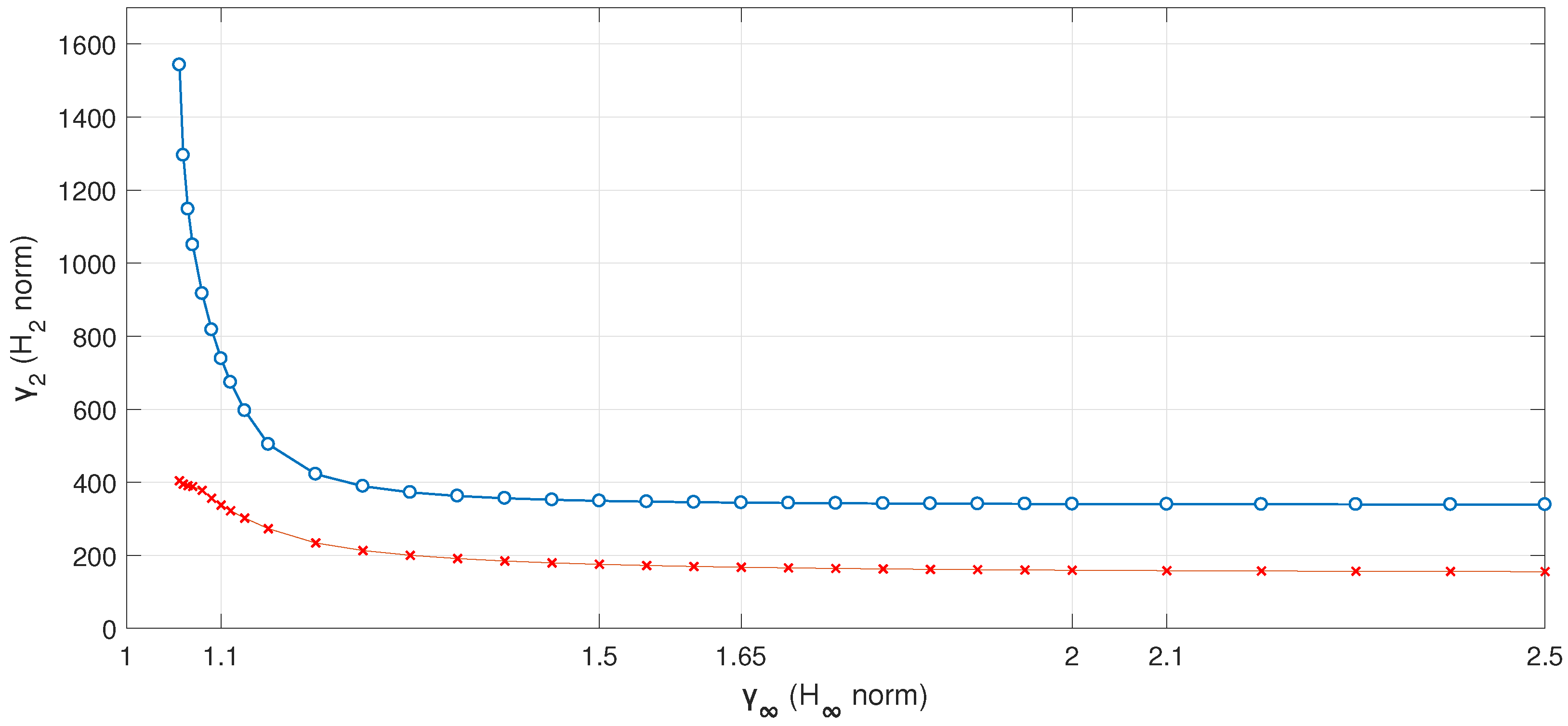
  • The second step is to estimate the scalar variable γ from above, more precisely to minimize the norm H 2 . Determining the relationship (Pareto curve) between the minimum value of the H 2 norm and the upper bound on the value of the H norm determined in the first step involves determining the range of scalar variables γ 2 that are the upper bound for the norm under study. In this example, the scalar variable γ 2 was tested in the range from [1.05:2.5] with a step of 0.05.
Below, a flow Figure 2 is presented that shows steps necessary for controller synthesis.
Points determined this way form the Pareto curve, where anything above the curve is a solution for which Criterion One H does not deteriorate Criterion Two H 2 . It is up to the user to decide which point in the region of acceptable solutions satisfies the intermediate assumptions regarding the control signal or static lag. If the set values of norms H 2 and H , obtained during synthesis of the state controller, are placed on or above the Pareto curve, this means that the desired controller for the current configuration, with the object, can be calculated using linear matrix inequalities. A solution to this problem was obtained with the help of multi-criteria optimization. One way is to use linear matrix inequalities. The synthesis of these norms is shown in the figure below Figure 3.

6. Results

A number of simulation studies have been performed. This article presents the research for two values of parameter γ and how it affects the dynamics of the system, operation of steering and propulsion equipment, and the trajectory of the training ship model “Blue Lady”. The study includes an analysis of the impact of choosing two different Pareto optimal solutions based on a pre-drawn plot of Pareto curves for two computational methods. The first method used a built-in MATLAB function called norm, and the second method was based on the relationships described in the subsections above. The study adopted the following research evaluation criteria:
1
Zero offset e ( t ) , shortest possible control time t r for a given control deviation value Δ u , v , r = 5 [%], no or small maximum overshoot M p (<5 [%] ).
2
Optimal control of steering and propulsion equipment, that is, minimizing energy consumption for the accomplishment of an assigned control task.
3
Obtaining a precise ship trajectory with no course fluctuations.
For each study, the analysis included:
  • Comparison of the reference signal with a controlled quantity together with quality criteria (such as control time a l p h a ) for three vessel speed components, u (longitudinal), v (lateral) and r (rotancional).
  • Impact of steering on propulsion and steering equipment, that is, minimizing fuel consumption and minimizing the impact of pollution on the marine environment.
  • Effect on plotted ship trajectory. Illustration of control precision accuracy.
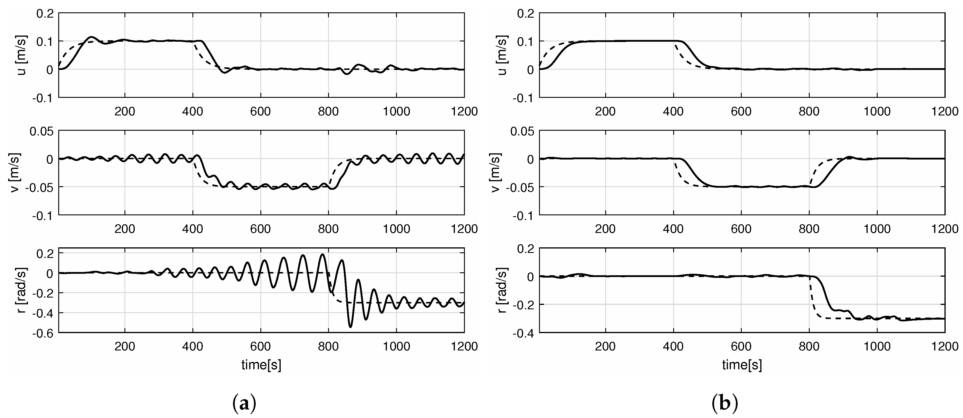
Figure 4 shows results of the performed complex manoeuvre, which consisted of three stages. Each stage took 400 [s], which makes up a total test time of 1200 [s]. In the first stage, forward motion was performed by controlling only longitudinal velocity u = 0.1 [m/s]. In the second stage, lateral movement was performed by setting longitudinal velocity u back to 0, while lateral velocity was set to v = 0.05 [m/s]. In the third and last stage, a stationary rotation was performed by setting lateral velocity v back to 0 and setting rotational speed r = 0.3 [rad/s].
Table 2 shows a comparison of control quality results obtained for the complex manoeuvre. Analyzing graphs of Figure 4, Figure 5, Figure 6 and Figure 7 for both γ coefficients for the complex manoeuvre, the following was noted in two subparagraphs:

6.1. Conclusions for γ = 1.1

For coefficient γ = 1.1 , during the complex manoeuvre, control time was obtained only for longitudinal speed u. This is due to the presence of oscillations for lateral velocity v and rotational velocity r.
-
Control system for rotational velocity r falls into increasing oscillations until time t = 800 [s], after which they begin to start decreasing, and at time t = 1000 [s] these oscillations are fully suppressed (oscillation amplitude = 0.05 u , v , r ).
-
This proves that the maximum overshoot obtained for rotational velocity is M p = 78.57 [%].
-
Thrusters operate in a chaotic way. For example, the rotation angle of thrusters (alfa d, alfa r) in a short time are changed from one swing limit to the opposite swing limit (from 120 to −120). Additionally, during the manoeuvre, the ship’s main propulsion system was switched on three times, which influenced the course of the speeds u, v, and r. In view of the above and in relation to the assumed test evaluation criteria, the dynamics of the tested system for γ = 1.1 does not meet the assumed criteria.
-
Controller force allocation is significant, especially the value of τ r in the range between [−250, 200], which significantly surpasses the amount of energy required by propulsion-control systems.

6.2. Conclusions for γ = 2.1

For coefficient γ = 2.1 , during the complex manoeuvre, control time was obtained for all three speed components, where for rotational speed r, control time of t = 180 [s] was achieved.
-
Oscillations are within the limits of the set value of control deviation only up to time t = 1047 [s], where after a time of 5 [s], the controlled quantity returns to the limits of control deviation and stabilizes. Nevertheless, the obtained value of maximum overshoot for rotational speed r was only 4.74 [%]. In addition, adjustment times of other speeds were short 118 [s] for longitudinal speed u and 104 [s] for lateral speed v, respectively.
-
For control waveforms of controlled devices, one can notice jumps in the controlled values at the moments of tasks of respective velocity components (t = 0; 400; 800 [s]). For lateral velocity task v, there are disturbances, which are the source of oscillations of thruster waveforms ( s s o d c , s s o r c ) and rotation angles of these thrusters (alfa d, alfa r ). In spite of this, thrusters gently change their state without consuming much energy. Oscillations of these quantities cease when speed-controlled quantity r returns into the limits of the set value of control deviation Δ r (t = 1047 [s]). This is the beginning of stabilization of the control system. During the whole manoeuvre, the main propulsion system was not switched on, which is in line with the optimum use of the ship’s propulsion and steering equipment.
-
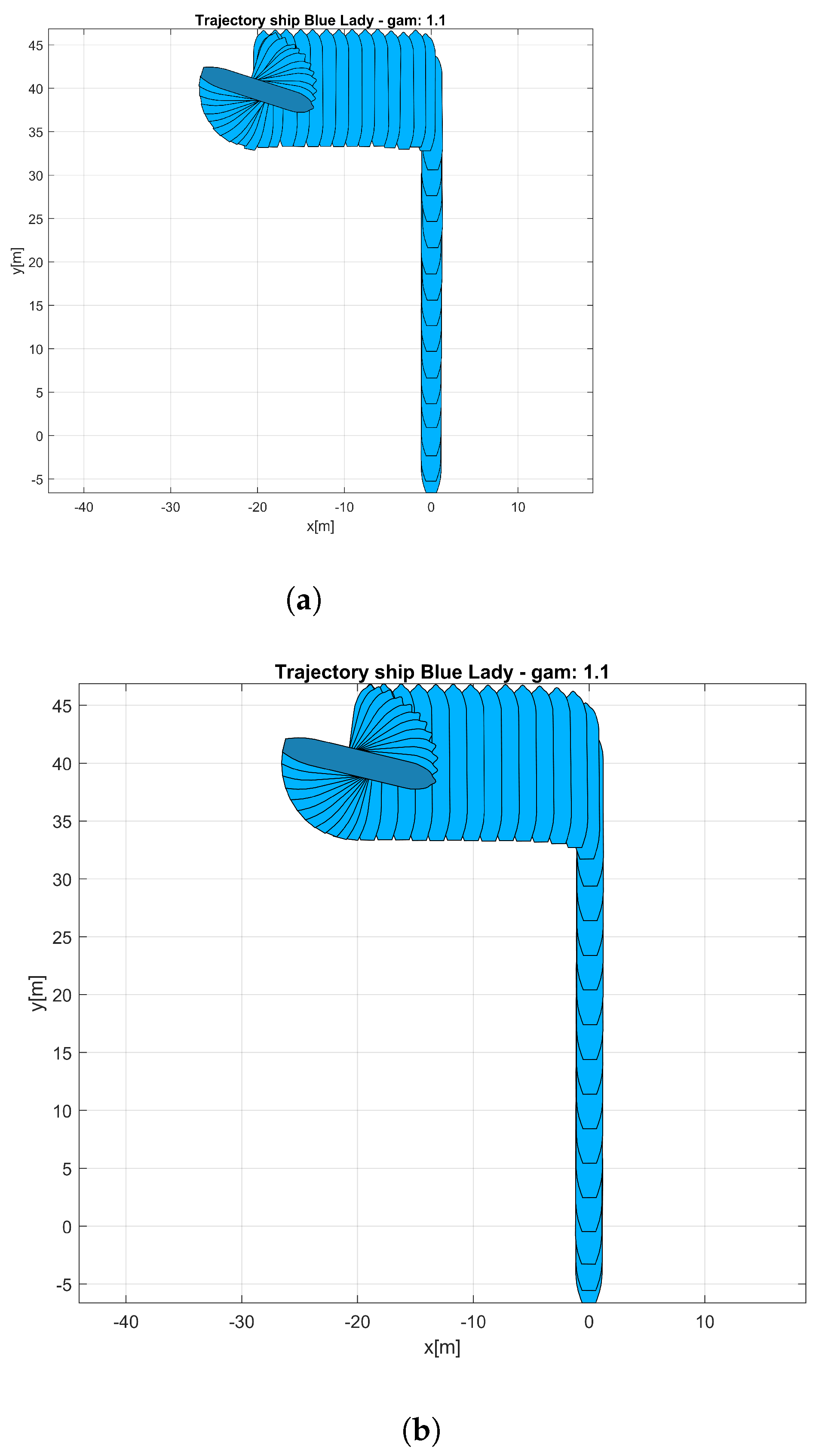
The ship’s trajectory is correct. To sum up, for the complex manoeuvre, the overshoot value was 4.74 [%]. Additionally, the values of determined deviations were equal or close to zero. In connection with the above and with reference to the assumed test evaluation criteria, the dynamics of the tested system for γ = 2.1 meets the assumed criteria.
-
Controller force allocation is acceptable in terms of the amount of energy required by by propulsion-control systems, and is in the range of [−60:60].

7. Conclusions

Optimization is a very broad topic, described in recent years in many fields, including the marine industry. It is proving to be an important criterion for the environment, as seen in a study on offshore [27] where a criterion of the electric propulsion system showed reduced fuel consumption (approx. 60 [%]). Sometimes it is difficult to get a compromise during research, where researchers from a completely different field pre-determine the minimization criteria and rather prove that optimization is not advisable in their work [28]. However, currently focusing on optimization in this work, the following has been demonstrated:
-
The γ coefficient has a significant influence on dynamics of the system, operation of steering and propulsion equipment and trajectory of the training ship model “Blue Lady”.
-
For the investigated multidimensional object, the best of the two selected values of γ coefficient turned out to be γ = 2.1 for complex manoeuvres.
-
After analysis of the results, it can be assumed that the closer the solution is to the OX abscissa axis, the worse the dynamics of the system.
-
For other multidimensional objects, the γ factor may differ significantly.
-
Obtained force values ( τ x , τ y , τ r ) prove that a properly selected value of γ optimizes energy required for propulsion and steering systems which, as per the authors, influences fuel savings of the ship.
In the research carried out, no rule for selection of the γ coefficient has emerged. The authors think that the best method of selection is the trial-and-error method, together with checking the dynamics of the system for each selected coefficient, as shown in the flowchart. In this case, the main aim of the research was to optimize the operation of propulsion and steering devices to reduce required energy and, as per the authors, also fuel consumption, while maintaining precise control the ship. It is also important to note that according to Pareto, everything that is above the curve is an acceptable solution; however, selection of proper values of γ and γ 2 has a major impact on the dynamics of propulsion and control systems of a ship model. Such a complex multicriterial function is difficult to achieve, and as such, the authors believe it is essential to observe the operation of propulsion and control systems during the controller synthesis process. The mathematical theory allows for some pre-selections; however, in automation applications, feedback is important, and this paper clearly shows that according to the Pareto theory, both values of γ are correct, but after observing the operation of propulsion and control systems, it is clearly seen that one is a significantly better choice for this specific control system. Due to the occurrence of uncertainties in the choice of the γ coefficient, the direction of further research could be to carry out tests on the same object with the synthesis of a controller based on neural networks with MOEA multi-criteria evolutionary algorithms, and to check what effect the choice of controller has on the choice of the γ coefficient.

Author Contributions

Conceptualization, M.R. and K.P.; methodology, K.P.; software, M.R.; validation, K.P.; formal analysis, M.R.; investigation, K.P.; resources, K.P.; data curation, M.R.; writing—original draft preparation, K.P.; writing—review and editing, M.R.; visualization, K.P.; supervision, M.R.; project administration, K.P.; funding acquisition, M.R. All authors have read and agreed to the published version of the manuscript.

Funding

The project is financed from the Ministry of Science and Higher Education program named “Regionalna Inicjatywa Doskonałości” in the years 2019–2022, project number 006/RID/2018/19, the sum of financing 11,870,000 PLN.

Institutional Review Board Statement

Not applicable.

Informed Consent Statement

Not applicable.

Data Availability Statement

Not applicable.

Acknowledgments

The authors want to thank the management and the technical staff of the Foundation for Safety of Navigation and Environment Protection in Iława, Poland, for their help and making the training ships available for the tests.

Conflicts of Interest

The authors declare no conflict of interest.

Abbreviations

The following abbreviations are used in this manuscript:
MDPIMultidisciplinary Digital Publishing Institute
DOAJDirectory of open access journals
TLAThree letter acronym
LDlinear dichroism

References

  1. Takahashi, R.; Palhares, R.; Dutra, D.; Goncalves, L. Synthesis and characterization of Pareto-optimal solutions for the mixed. In Proceedings of the IEEE Conference on Decision and Control, Orlando, FL, USA, 4–7 December 2001. [Google Scholar]
  2. Takahashi, R.; Palhares, R.; Dutra, D.; Goncalves, L. Estimation of Pareto sets in the mixed H2/H control problem. Int. J. Syst. Sci. 2004, 35, 55–67. [Google Scholar] [CrossRef]
  3. Sánchez, G.; Villasana, M.; Strefezza, M. Multi-objective Pole Placement with Evolutionary Algorithms. In Proceedings of the International Conference on Evolutionary Multi-Criterion Optimization, Matsushima, Japan, 5–8 March 2007. [Google Scholar]
  4. Poussot-Vassal, C.; Sename, O.; Dugard, L.; Gaspar, P.; Szabo, Z.; Bokor, J. The design of a chassis system based on multi-objective qLPV control. J. Transp. Eng. 2008, 36, 93–97. [Google Scholar] [CrossRef] [Green Version]
  5. Zhang, Z.; Qian, S. Multi-objective Immune Optimization in Dynamic Environments and Its Application to Signal Simulation. In Proceedings of the International Conference on Measuring Technology and Mechatronics Automation, Changchun, China, 9–12 August 2009. [Google Scholar]
  6. Bal, D.; Kogan, M. Multi-Objective Generalized H2 Control for Optimal Protection from Vibration. In Proceedings of the UKACC 12th International Conference on Control, Sheffield, UK, 5–7 September 2018. [Google Scholar]
  7. Balandin, D.V.; Kogan, M. Pareto suboptimal controllers in multi-objective disturbance attenuation problems. Automatica 2017, 84, 56–61. [Google Scholar] [CrossRef]
  8. Balandin, D.; Biryukov, R.; Kogan, M. Localization of Pareto-Optimal Set in Multi-objective Minimax Problems. In Proceedings of the International Conference on Mathematical Modeling and Supercomputer Technologies, Nizhny Novgorod, Russia, 23–27 November 2020. [Google Scholar]
  9. GÜnes, F.; Uluslu, A.; Mahouti, P. Pareto Optimal Characterization of a Microwave Transistor. IEEE Access 2020, 8, 47900–47913. [Google Scholar] [CrossRef]
  10. Le, T.A.; Chien, T.V.; Nakhai, M.R.; Le-Ngoc, T. Pareto-Optimal Pilot Design for Cellular Massive MIMO Systems. IEEE Trans. Veh. Technol. 2020, 69, 13206–13215. [Google Scholar] [CrossRef]
  11. Rybczak, M. Synteza Elektronawigacyjnego Układu Wielowymiarowego Sterowania Statkiem Wykorzystująca Liniowe Nierówności Macierzowe; Uniwersytet Morski w Gdyni: Gdynia, Poland, 2020. [Google Scholar]
  12. Gierusz, W.; Rybczak, M. Effectiveness of Multidimensional Controllers Designated to Steering of the Motions of Ship at Low Speed. Sensors 2020, 20, 3533. [Google Scholar] [CrossRef] [PubMed]
  13. Miller, A.; Rybczak, M.; Rak, A. Towards the Autonomy: Control Systems for the Ship in Confined and Open Waters. Sensors 2021, 21, 2286. [Google Scholar] [CrossRef] [PubMed]
  14. Tomera, M. Swarm intelligence applied to identification of nonlinear ship steering model. In Proceedings of the 2015 IEEE 2nd International Conference on Cybernetics (CYBCONF), Gdynia, Poland, 24–26 June 2015; pp. 133–139. [Google Scholar]
  15. Kula, K.S.; Tomera, M. Control system of training ship keeping the desired path consisting of straight-lines and circular arcs. Int. J. Mar. Navig. Saf. Sea Transp. 2017, 11, 711–719. [Google Scholar] [CrossRef] [Green Version]
  16. Tomera, M. Path Controller for Ships with Switching Approach. In Advanced, Contemporary Control; Springer: Cham, Switzerland, 2020; pp. 1519–1530. [Google Scholar]
  17. Boyd, S.; El Ghaoui, L.; Feron, E.; Balakrishnan, V. Linear Matrix Inequalities in System and Control Theory; Society for Industrial and Applied Mathematics (SIAM): Philadelphia, PA, USA, 1994; Volume 15. [Google Scholar]
  18. Duan, G.R.; Yu, H. Linear Matrix Inequalities in Control Systems: Analysis, Design and Applications; CRC Press: Boca Raton, FL, USA, 2013. [Google Scholar]
  19. Galas, Z.; Nykowski, I.; Zolkiewski, Z. Programowanie wielokryterialne. In Państwowe Wydawnictwo Ekonomiczne; Państwowe Wydawnictwo Ekonomiczne: Warsaw, Poland, 1987. [Google Scholar]
  20. Kaliszewski, I. Wielokryterialne Podejmowanie Decyzji: Obliczenia MięKkie dla ZłożOnych Probelmów Decyzyjnych; Wydawnictwo Naukowo—Techniczne: Katowice, Poland, 2008. [Google Scholar]
  21. Lisowski, J. Computational intelligence methods in the safe ship control process. Pol. Marit. Res. 2001, 8, 18–24. [Google Scholar]
  22. Lisowski, J.; Mohamed-Seghir, M. Comparison of Computational Intelligence Methods Based on Fuzzy Sets and Game Theory in the Synthesis of Safe Ship Control Based on Information from a Radar ARPA System. Remote Sens. 2019, 11, 82. [Google Scholar] [CrossRef] [Green Version]
  23. Sultan, K.S.; Emam, W. The Combined-Unified Hybrid Censored Samples from Pareto Distribution: Estimation and Properties. Appl. Sci. 2021, 11, 6000. [Google Scholar] [CrossRef]
  24. Scherer, C.i.; Wieland, S. Linear Matrix Inequalities in Control Lecture Notes; Dutch Institute for Systems and Control: Delft, The Netherlands, 2000. [Google Scholar]
  25. Sturm, J.F. Using sedumi 1.02, a matlab toolbox for optimization over symmetric cones. Optim. Methods Softw. 1999, 11, 625–653. [Google Scholar] [CrossRef]
  26. Ravat, A.K.; Dhawan, A.; Tiwari, M. LMI and YALMIP: Modeling and Optimization Toolbox in MATLAB. In Advances in VLSI, Communication, and Signal Processing; Springer: Singapore, 2021; pp. 507–515. [Google Scholar]
  27. Łebkowski, A. Analysis of the use of electric drive systems for crew transfer vessels servicing offshore wind farms. Energies 2020, 13, 1466. [Google Scholar] [CrossRef] [Green Version]
  28. Gong, Z.; Zhong, P.; Hu, W.; Hua, Y. Joint Learning of the Center Points and Deep Metrics for Land-Use Classification in Remote Sensing. Remote Sens. 2019, 11, 76. [Google Scholar] [CrossRef] [Green Version]
Figure 1. (a) Blue Lady 3D ship model. (b) Actual Blue Lady ship model on Silm lake. Ship parameters: Lenght 13.75 [m], width 2.38 [m].
Applsci 11 07297 g001
Figure 2. State controller synthesis method.State controller synthesis method.
Applsci 11 07297 g002
Figure 3. Graph of obtained Pareto curves for the studied control system. Blue line—Matlab algorithms, red line—calculations using YALMIP and SeDuMi libraries with LMI conditions [25,26].
Applsci 11 07297 g003
Figure 4. The three components of vessel speed, u, v, and r. Reference value (dashed line), regulated quantity (solid line). For two Pareto optimal solutions: (a) γ = 1.1, (b) γ = 2.1.
Applsci 11 07297 g004
Figure 5. Command diagrams for individual steering and propulsion devices. For two Pareto optimal solutions: (a) γ = 1.1, (b) γ = 2.1.
Applsci 11 07297 g005
Figure 6. Trajectory of the ship while performing the complex manoeuvre. Initial course of vessel = 0 [deg]. For two Pareto optimal solutions: (a) γ = 1.1, (b) γ = 2.1.
Applsci 11 07297 g006
Figure 7. Controlled object has three input signals: τ x ; τ y ; τ r , where: [ τ x ]—required force (thrust) on the ships longitudinal axis, [ τ y ]—required force (thrust) on the ships lateral axis, [ τ r ]—required rotational force. (a) γ = 1.1, (b) γ = 2.1.
Applsci 11 07297 g007
Table 1. Input signals of propulsion and control devices of the “Blue Lady” ship model.
SymbolName of SignalRangeUnit
ngMain propeller rotational speed(−200; +480)[rpm]
deltaRudder deflection angle(−35; +35)[deg]
sstdRelative thrust of the bow tunnel thruster(−1, +1)[-]
sstrRelative thrust of the stern tunnel thruster(−1, +1)[-]
ssodRelative thrust of the bow rotary thruster(0, +1)[-]
alfa dBow rotary thruster deflection angle(−120, +120)[deg]
ssorRelative thrust of the stern rotary thruster(0, +1)[-]
alfa rStern rotary thruster deflection angle(−120, +120)[deg]
Table 2. Comparison of control quality results obtained for the complex manoeuvre.
Longitudinal uLateral vRotational r
Parameter1.12.11.12.11.12.1
t r [s]163118104180
M p [%]15.040.919.901.9278.574.74
e ( t ) [m/s]000000
t n [s]406555605495
Publisher’s Note: MDPI stays neutral with regard to jurisdictional claims in published maps and institutional affiliations.