Study of the Optimal Waveforms for Non-Destructive Spectral Analysis of Aqueous Solutions by Means of Audible Sound and Optimization Algorithms

Abstract

Acoustic analysis of materials is a common non-destructive technique, but most efforts are focused on the ultrasonic range. In the audible range, such studies are generally devoted to audio engineering applications. Ultrasonic sound has evident advantages, but also severe limitations, like penetration depth and the use of coupling gels. We propose a biomimetic approach in the audible range to overcome some of these limitations. A total of 364 samples of water and fructose solutions with 28 concentrations between 0 g/L and 9 g/L have been analyzed inside an anechoic chamber using audible sound configurations. The spectral information from the scattered sound is used to identify and discriminate the concentration with the help of an improved grouping genetic algorithm that extracts a set of frequencies as a classifier. The fitness function of the optimization algorithm implements an extreme learning machine. The classifier obtained with this new technique is composed only by nine frequencies in the (3–15) kHz range. The results have been obtained over 20,000 independent random iterations, achieving an average classification accuracy of 98.65% for concentrations with a difference of ±0.01 g/L.

1. Introduction

Acoustic spectroscopy is one of the most promising techniques for nondestructive testing of many materials. This work shows that acoustic spectroscopy in the audible range is also well prepared for the study of liquid solutions. No method can claim superiority, but sound-based sensing of liquids has several advantages over optical techniques and can be easily combined with other methods, such as electroacoustic measurements, as discussed in [1]. A review devoted to describing the advantages and limitations of acoustic spectroscopy, with a particular focus on pharmaceutical applications can be seen in [2].

However, most studies on this research topic are devoted to ultrasound techniques and devices, due to their higher energy and bandwidth than sounds in the audible range. This can be seen in the monographs devoted to this topic, like [3] and [4]. The last one is very interesting because a research by Contreras et al. [5], page 51, describes the ultrasonic measurement of different sugar concentrations with an accuracy of 0.2% in water volume for pure sugar solutions. They measured the velocity of ultrasound and the density in solutions of D-glucose, D-fructose, and sucrose at various concentrations (0–40% w/v) and temperatures (10–30 °C).

This conversion of acoustic data to sound velocity is the norm in most ultrasound studies of liquids. The calculation of sound velocities introduces some important problems and uncertainties due to the need of using statistical or theoretical models and the existence of other processes, as is explained in several publications, for example the Dzida et al.’s excellent review about the determination of the speed of sound in ionic liquids [6]. A description of a low-cost system for the measurement of sound velocity in liquids can be found in [7].

The use of ultrasound for the study of pure liquids and solutions is limited, com-pared to its application to colloids, suspensions, and emulsions, as reviewed in [8]. However, there have been remarkable advances in recent years, as can be seen, for example, in [9,10,11,12]. The acoustic research of aqueous electrolytes was performed by Pal and Roy in [13] using the Fourier spectrum pulse-echo technique, which is discussed in detail in [14].

The number of publications is too large for an exhaustive literature survey, so only a handful of representative examples are shown here. For a detailed review of ultrasound spectroscopy for particle size determination see [15]. In [16] Silva et al. studied polydisperse emulsions by means of acoustic spectroscopy within the frequency range of (6–14) MHz in order to measure the droplet size distribution of water-in-sunflower oil emulsions for a volume fraction range from 10 to 50%. They concluded that the methodology was suitable for polydisperse particle size characterization for moderate concentrations up to 20% and the results were in good agreement with those obtained by laser diffraction analysis. Other interesting application to food analysis can be seen in [17], where the mechanism of rehydration of milk protein concentrate powders is studied by means of broadband acoustic resonance dissolution spectroscopy. Moreover, ref. [18] describes the use of an ultrasonic pulse echo system for vegetable oils characterization.

Good reviews of high-resolution ultrasound spectroscopy can be found in [19,20]. All measurements are based on the previous determination of the speed of sound and attenuation in the samples. A number of advantages and applications of this technique are clearly described, for example, samples with very small volumes can be analyzed using different ranges of pressure and temperature. As is explained in [19], at frequencies below 100 MHz, which is clearly the case of audible frequencies, for nano-sized dispersions or solutions, the contribution of scattering to attenuation can be neglected. Thus, attenuation at this long-wavelength regime is determined by the thermal and the shear (visco-inertial) effects. In spite of this, we show that audible acoustic spectroscopy can achieve impressive accuracy in the determination of fructose concentration in water.

Another interesting application of ultrasound spectroscopy is the monitoring of biocatalysis in solutions and complex dispersions, even in real-time, reviewed in detail by Buckin and Caras in [21]. The information that can be extracted from ultrasound data is impressive: substrate concentrations along the entire course of the reaction, time profile analysis of the degree of polymerization, reaction rate evolutions, kinetic mechanism evaluation, kinetic and equilibrium constant measurements, and real-time traceability of structural changes in the medium associated with chemical reactions, among others.

Finally, an interesting and fascinating application of audible acoustic measurements can be found in [22,23]. Both deal on the determination of Martian rock properties using the microphone of the recent NASA Perseverance rover. This microphone is used to record the sounds associated with the microcrater-forming laser induced breakdown spectroscopy device shots.

Additionally, artificial intelligence (AI) algorithms have been incorporated into many engineering applications in recent years. They are integrated in research always providing a remarkable improvement in performance and efficiency. The use of these algorithms is enhanced by continuous and increasing computing power and massive data collection. Although they do not always offer the optimal solution, they approach it with a very acceptable balance of cost and accuracy. Moreover, in many applications there is no unique solution, but rather several solutions under conflicting criteria. Recent studies on the application of IA in different fields of engineering can be found in: computer engineering [24,25,26,27], electrical engineering [28,29], petroleum engineering [30], fluid mechanic engineering [31,32], energy engineering [33,34,35,36], and acoustic engineering [37].

In this work a direct application of audible acoustic spectroscopy to the determination of fructose concentrations in distilled water is presented. It is shown that no data conversion to speeds of sound is necessary, hence eliminating the source of some uncertainty, and most importantly, accuracies of the order of 1 part in 100,000 (0.001%) in weight can be achieved. The use of audible sound has some advantages over ultrasound, mainly the low cost of the measuring equipment and the noncontact nature of the measurements. In order to optimize the technique, the results from a series of different pulses and noises were previously compared and the best sound was selected for the final determination. This is a clear improvement over our previous technique based on resonant vibrations of the sample, which involved direct contact [38].

In this work, 364 samples of different concentrations of high purity fructose in distilled water were used for the study of the best pulse characteristics for acoustic chemical analysis. A constant volume of 150 mL for all samples was selected. The container was a simple cylindrical glass. A small anechoic chamber was used to place the samples and to make the sound recordings. The microphone was placed vertically over the surface of the liquid. The sound source was one earpiece placed parallel to the microphone over the liquid surface.

Different sound configurations were explored: chirp, square pulses, white noise, and maximum length sequence (MLS). In the end, MLS produced the best results in our preliminary studies and was selected for the final analysis. The samples were excited by these sounds during 30 s intervals and the reflected sound was recorded. These recordings were divided into 2-s samples whose spectra were calculated by means of the Praat program [39]. The resulting spectra were processed by means of a grouping genetic algorithm (GGA) taking a training set of 80% and a test set of 20%. This algorithm provided a classifier with more than 98.5% classification accuracy, even for concentrations with a difference of ±0.01 g/L.

2. Materials and Methods

The experimental system was composed of three main parts: the anechoic chamber, the sound system, and the samples. The liquid sample was placed inside a small handmade anechoic chamber of exterior dimensions (width, high, depth) 80 × 72 × 56, in centimeters. Its interior was isolated using 2-cm thick foam and a frequency-dependent absorbent pyramidal material of 4 cm in the base and 6 cm high. Thus, the interior volume of the chamber is 58 × 61 × 40 cm. A cylindrical glass with a volume of 200 mL filled with 150 mL of a water and fructose solution was placed at the center of the chamber. The glass mass was 123 g, with a diameter of 8 cm. Figure 1 shows the schematic diagram of the experimental setup.

The proposed method uses differential measurements and the acoustic performance of the chamber and the environment is sufficient for this purpose. Measurements of the chamber performance were made by means of a Brüel and Kjaer 2250 acoustic analyzer, resulting in 28.2 dBA of background noise and a mean reverberation time of 0.17 s. The frequency response of the chamber is represented in Figure 2.

The used microphone was the model ECM-TL3 of Sony, an electret capacitor with omnidirectional pattern, frequency response range (20 Hz–20 kHz) with sensitivity of −35 dB that was placed vertically 2.5 cm over the liquid surface, 1.5 cm from the center. In parallel, in a symmetric position to the center of the glass, one earpiece model Sony MDRXB50APB.CE7 was used as the sound source, with a frequency response range of (4–24) kHz, a sensitivity of 106 dB/mW, and an impedance of 40 ohms (1 kHz). The test signals were generated by a computer while the recordings were made by another computer and an external audio card.

The measuring system, background sound, and noise sound generated by the sound card is represented in Figure 3. A maximum level of 0.0271 is measured against the levels near 1 (to full scale) of the signals.

The microphone was connected to a PC sound card MAudio Fast Track Ultra 8R. An amplification factor of 70% for the channel was used to avoid adding internal noise from the card. The measurements were taken with a recording rate of 44.1 kHz by means of the free Audacity software [40]. Sound amplitude was kept below the 70% of the maximum level in order to avoid saturation effects. Some test signals were generated by MATLAB [41] and Audacity software:

• MLS signal: a signal generated by MATLAB, taking into account that the maximum length is 30 s. The amplitude is 60% of the full scale (FS);
• White noise: a signal generated by Audacity, with an amplitude of 60% of the FS;
• A set of chirp signals generated by Audacity, with a duration of 1 s each, from 150 Hz to 15 kHz;
• Square pulses with a period of 250 ms and 50% of duty cycle.

Each audio recording had a duration of 30 s, more than enough to ensure the precision and stability of the measurements. Later analyses showed that the recordings were stable enough to allow their partition in several 2 s intervals in order to increase the number of recordings for the classification algorithm. Changes among different spectra from the same sample were so low that they were not measurable.

The experiments were performed with a set of 364 samples of water solutions with different concentrations of fructose (see

Table 1. Number of samples and their composition used in the experiment. A total of 130 samples of distilled water with different concentrations of fructose, in the range of 0 g/L to 9 g/L, were analyzed.

Fructose Concentration (g/L)	0	1	2	3	4	5	6	7	8	9
Number of samples	13	13	13	13	13	13	13	13	13	13
Total samples	130

,

Table 2. Number of samples and their composition used in the experiment. A total of 117 samples of distilled water with different concentrations of fructose, in the range of 2.1 g/L to 2.9 g/L, were analyzed.

Fructose Concentration (g/L)	2.1	2.2	2.3	2.4	2.5	2.6	2.7	2.8	2.9
Number of samples	13	13	13	13	13	13	13	13	13
Total samples	117

and

Table 3. Number of samples and their composition used in the experiment. A total of 117 samples of distilled water with different concentrations of fructose, in the range of 2.01 g/L to 2.09 g/L, were analyzed.

Fructose Concentration (g/L)	2.01	2.02	2.03	2.04	2.05	2.06	2.07	2.08	2.09
Number of samples	13	13	13	13	13	13	13	13	13
Total samples	117

). The volume of each sample was 150 mL. Distilled water was used as solvent. Food grade pure fructose (>99%) was used for the liquid samples. The concentrations of fructose were from 0 to 9 g/L. A more detailed study was done between 2 g/L and 3 g/L in increments of ±0.1 g/L and between 2.01 g/L and 2.09 g/L in increments of ±0.01, in order to explore the performance of the system. The mass of fructose was measured by means of an analytical balance, a Homgeek TL-Series balance with an accuracy of 50 g/0.001 g.

A set of 130 samples of water and fructose solutions with 10 concentrations between 0 g/L and 9 g/L, 117 samples of water and fructose solutions with 9 concentrations between 2 g/L and 3 g/L, 117 samples of water and fructose solutions with 9 concentrations between 2.0 g/L and 2.1 g/L have been analyzed inside an anechoic chamber using audible sound configurations.

Samples were numbered and visual inspection was used in order to ensure that complete dilution was achieved, and no bubbles were formed. Careful manipulation of the samples was done in order to avoid the formation of bubbles or wall drops. Each measurement took 30 s and they were taken in a consecutive way.

Each measurement was divided into different 2-s intervals, after verifying that such time was more than enough for accurate and precise spectral information. The input data of the classification algorithm are the spectra of the audio measurements of 2-s in duration. The experiment was carried out with one audio measurement of each of the 28 different concentrations. That means a total of 364 audio samples. The power spectrum of every interval was made using the default Praat 6.0.40 options as can be seen in our previous work [38]. Similarly, a cepstral smoothing of 100 Hz and a decimation procedure were applied (65,537 points); averaged in order to reduce the number of points to a reasonable size (655 points) without losing the main peak structure of the spectra. In summary, the classification algorithm processed 364 input data, each of them being a spectrum defined by 655 values in the frequency range (20 Hz–22.05 kHz).

3. Algorithm for Clustering Problem

The spectral response of the liquid samples to the vibrational stimulation of the MLS sounds was used as data input to a genetic grouping algorithm (GGA) to perform the classification of the liquid mixtures according to their fructose concentration. Since the nature of the samples was not affected, it is a non-destructive method. The GGA is itself a genetic algorithm (GA) explicitly modified for solving clustering problems. A brief description of GAs and GGAs is given in this section.

3.1. From Genetic Algorithm to Grouping Genetic Algorithm

GA is a bio-inspired algorithm based on the theory of evolution of species by natural selection. A population of individuals fights against each other to gain the resources to survive. Each individual represents an encoded solution of the optimization problem. It is therefore an evolutionary optimization algorithm. The optimization strategy is usually applied to solve problems where it is almost impossible to find the optimal solution and there are several solutions with opposing criteria. The objective is to find one or multiple solutions which are close enough to the optimal one, with a very acceptable balance between cost and accuracy. On the other hand, “evolutionary” means that the algorithm computes the solutions through successive generations, undergoing an evolutionary process that enhances an overall improvement in the fitness value of the majority. Individuals with better fitness values are likely to survive longer than individuals with worse fitness. Along successive generations, individuals will appear that are more fit than others and will progressively improve their fitness. Each generation of individuals undergoes changes through recombination, mutation, and selection functions. These functions allow the diversity of individuals and therefore the exploration of the solution space. The execution of the evolutionary algorithm is completed when it reaches a stop condition. The most popular stopping conditions are a maximum number of generations and population convergence. Population convergence is reached when there is no progress in improving the fitness of individuals over several consecutive generations. A more extensive introduction can be found in [42].

The GGA is a modification of the GA oriented to solve grouping and clustering problems [43,44,45,46]. The fundamental difference of a GGA versus a GA lies in the encoding of the solution and the use of search operators to manage this encoding. The encoding is key to ensuring high performance in the execution of the algorithm [47]. A solution in the GGA is composed of two sections: the assignment part and the grouping part. The grouping section labels all the groups involved in the solution. The assignment part associates each element to a single group. The value stored in the assignment part is the group assigned to each element. The information about the grouping is in the content of the solution itself and in its length. The total length of the solution is the number of elements to be classified plus the number of groups considered in the solution.

3.2. The Fitness Function: The Extreme Learning Machine

The fitness function numerically characterizes the individual and allows to rank the individuals of a population from best to worst aptitude. The fitness function used in the GGA is the extreme learning machine (ELM). It is a relatively simple machine learning algorithm that generalizes a single hidden layer feedforward network (SLFN), used for regression, binary classification, and multi-classification [48,49,50,51,52,53]. The input layer takes the input values for a given set of features from the data. The feature set can include all the features of the data or a subset of them. The output layer provides a classification of the data according to the fixed feature set. The single intermediate layer is adjusted by the training of the network. After training, the classification accuracy of the ELM is calculated according to the defined feature set. ELM has demonstrated good performance with extremely high speed [54,55,56]. This last feature is fundamental for its integration in the GGA, since an extremely high number will be executed during each generation of the evolutionary algorithm.

The fitness function is applied to an individual by calculating by ELM the classification accuracy of each of the groups considered in the solution. The best rate is assigned as the fitness value to the individual and the classification rates of the rest of the groups are then discarded. The best classification accuracy corresponds to the group of features that classifies the individual with the best accuracy among all the groups considered in the solution. The rest of the groups are not relevant to the solution.

3.3. Metaheuristic GGA+ELM Algorithm Application for Spectral Analysis

As already mentioned, the spectral data have 655 values in the frequency range (20 Hz–22.05 kHz). Obviously 655 characteristics is far too high for classification purposes. The target of the optimization algorithm is to reduce the number of features useful for classifying liquid samples. This means a wrapper feature selection [57] where the GGA maximizes the classification accuracy. The solution is composed of a collection of features varying in length and composition. The set of features extracted by the GGA among the 655 total will constitute the classifier applicable on the spectra of the liquid samples. The challenge is to not exceed more than 10 features and to achieve a classification accuracy of more than 95%.

The training and testing data sets are disjoint sets randomly selected from the total of samples. The usual ratio is 80/20, with the training set having the largest number (80%) and the test data the remaining 20%. The population size usually used in the literature varies between 20 and 100 [58,59]. The pair composition of individuals for the crossover operation is randomized. This method has also provided good results in previous research [60,61]. The crossover operation generates a population increase of 50% (a single offspring from each pair), on which a 10% mutation is applied [47,59]. This percentage is higher than usual in genetic algorithms, with the purpose of quickly exploring multiple areas of the solution space. The survival population for the next generation is composed of the winners of pairwise tournaments among the total population. The matches are chosen randomly. The fitness function value of the fighters determines the winner of each tournament.

As already described, an individual is coded as a set of groups, where each group is a collection of features that can be a valid classifier of the input data. Not all groups of an individual are useful for classification, but only those with better accuracy. Note that considering a specific individual, each feature of the 655 is only present in a single group. In the GGA fitness function, the ELM algorithm is applied over each group of the individual to classify the testing set data from the knowledge of the training data. The group with the best classification accuracy is selected as a candidate classifier. The fitness of the individual takes the value of the classification accuracy of this highlighted group, which is the best accuracy obtained among all the groups of the individual.

The stopping condition employed in optimization is the maximum number of generations. To ensure the high-quality solutions are found within a reasonable computation time, the maximum number of genera considered is G_max = 50.

4. Results and Discussion

The spectral analysis was performed on a total of 364 spectra from 28 different fructose contents, having 13 samples of each concentration. The 28 concentrations have been grouped into three data tables with their respective fructose concentration increments: ±1 g/L in Table 1, ±0.1 g/L in Table 2, and ±0.01 g/L in Table 3. The algorithm was run on the three sample collections. One purpose of this work is to obtain a limited set of frequencies able to satisfactorily classify the samples according to their concentration. The main objective is to determine the degree of discrimination of the classifier on fructose concentration using this method. It is expected that the accuracy classification of samples in Table 3 will be lower than the accuracy classification of samples in Table 1, as in Table 3 the concentration increment is much lower than in Table 1. It is also desired to know whether the accuracy classification of concentrations with a difference of ±0.01 g/L is acceptable or not.

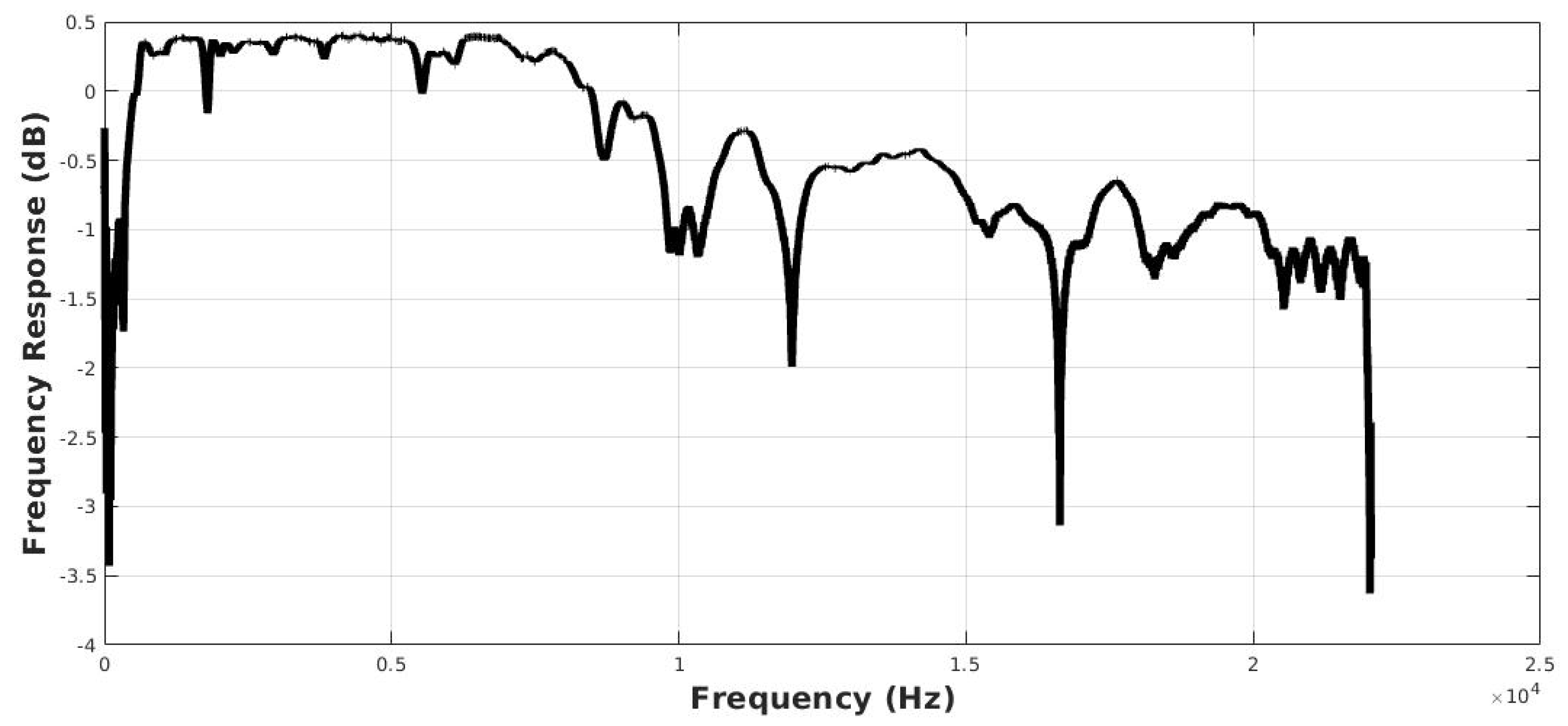
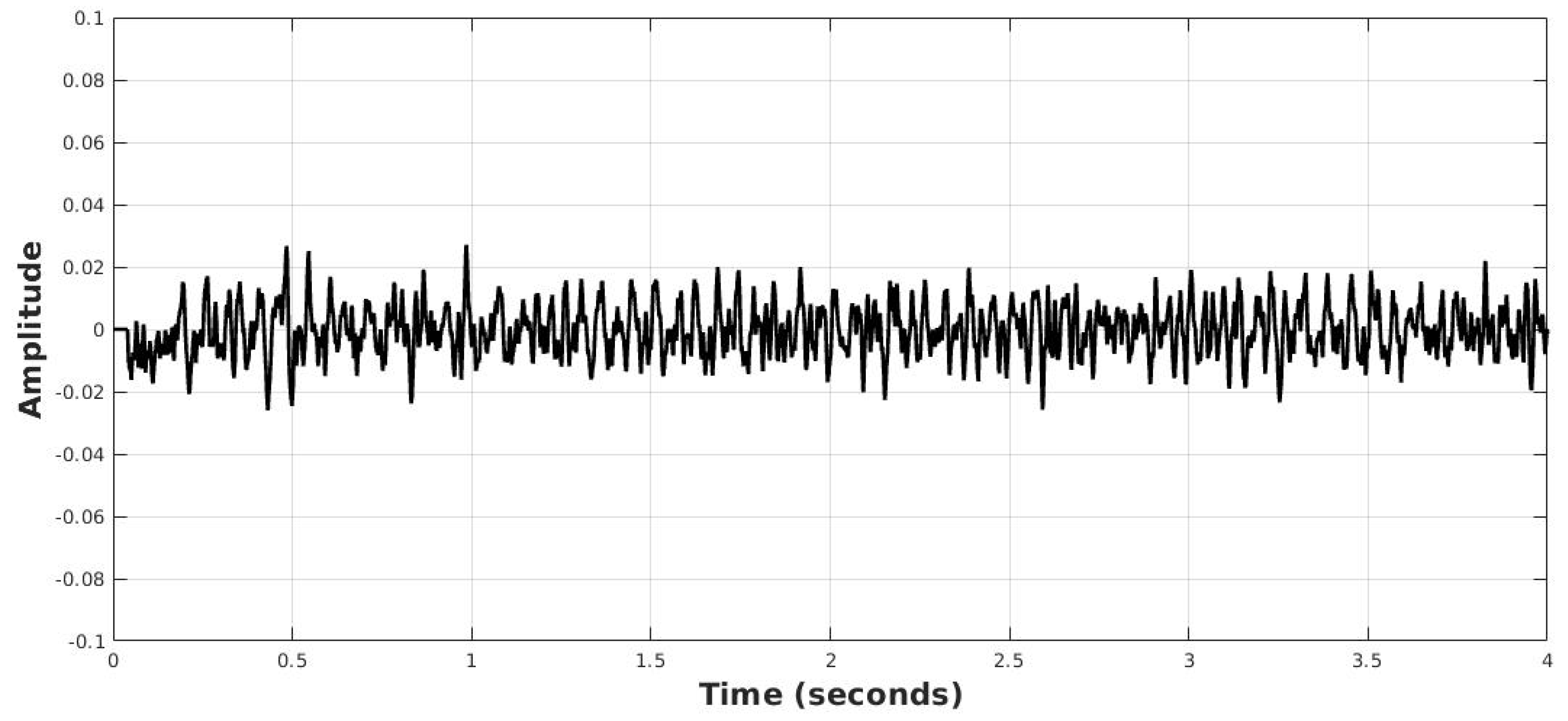
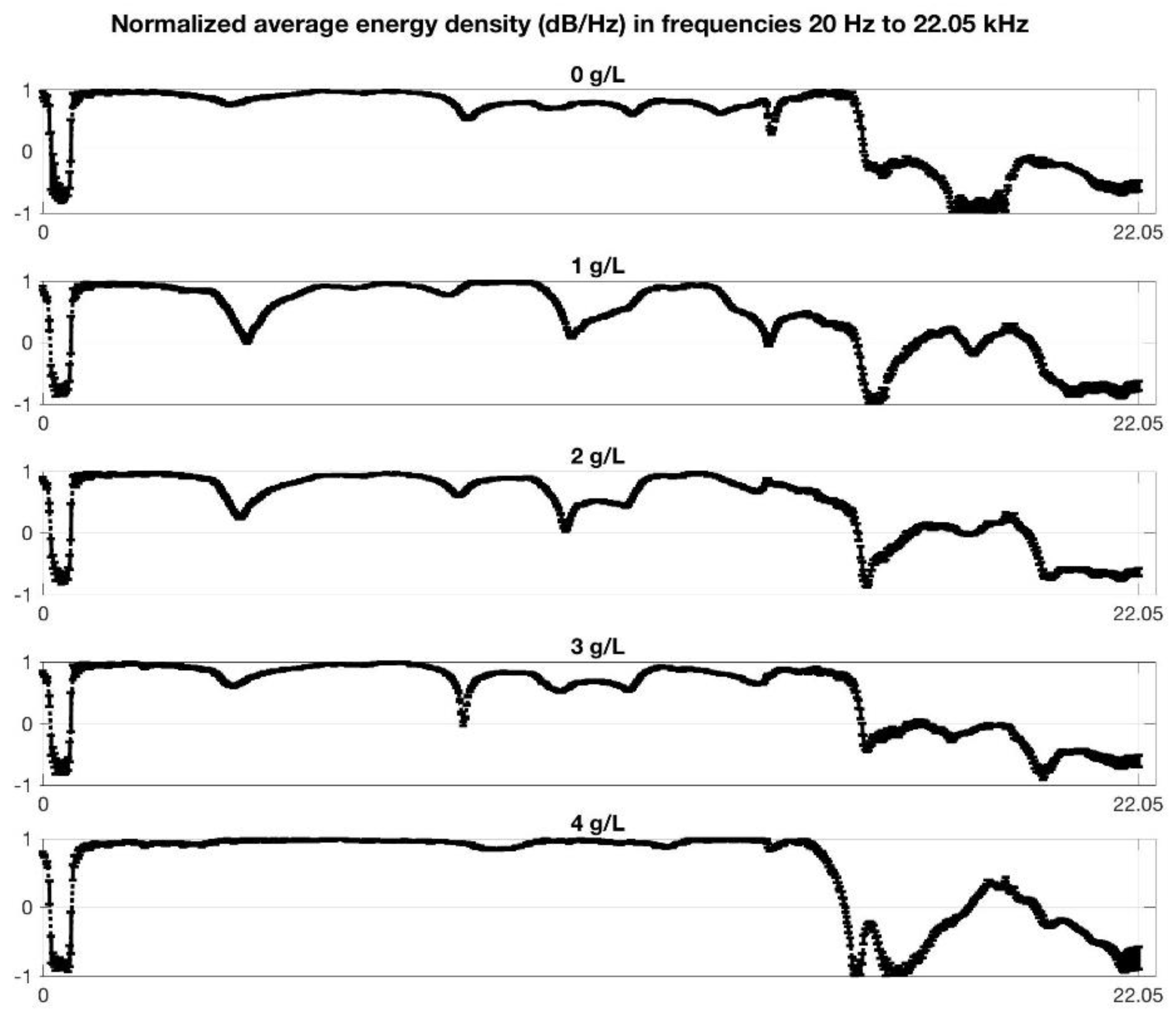
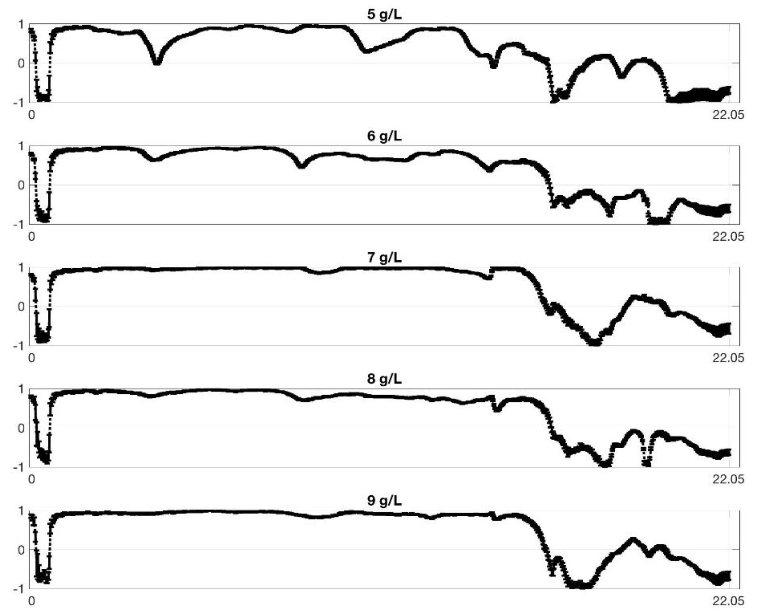
4.1. Acoustic Response Spectrum

Figure 4 shows the averaged spectra for each concentration from Table 1. The spectra are defined by the sound pressure level (dB/Hz) over the audible frequencies range (20 Hz–22.05 kHz). The sound pressure level is normalized in all the curves in Figure 4, with values in the range (−1–1).

Each spectrum can be characterized by particular markers associated with the chemical composition of the mixture. The selection of a group of frequencies manually as a classifier of liquid mixtures from their concentration is a tedious and complex task because of the large number of spectral lines (the algorithm handles the range of audible frequencies as 655 spectral lines).

The average spectra obtained with the samples from Table 2 and Table 3 also show a high complexity. Among the mean spectra from Table 3, with increments of 0.01 g/L, some of them are relatively similar to each other, and it may be necessary to select more focused frequency ranges to discriminate one concentration from another.

The optimization algorithm was run separately for each sample collection (Table 1, Table 2 and Table 3) providing several solutions. Each solution was composed of a set of frequencies that classify the samples with high accuracy. Two of these solutions were then taken to compose a combined decision system. This combined classifier works as a unique and common classifier over all samples used. In the following lines, the performance of this classifier on samples with concentrations from Table 1, Table 2 and Table 3 is analyzed.

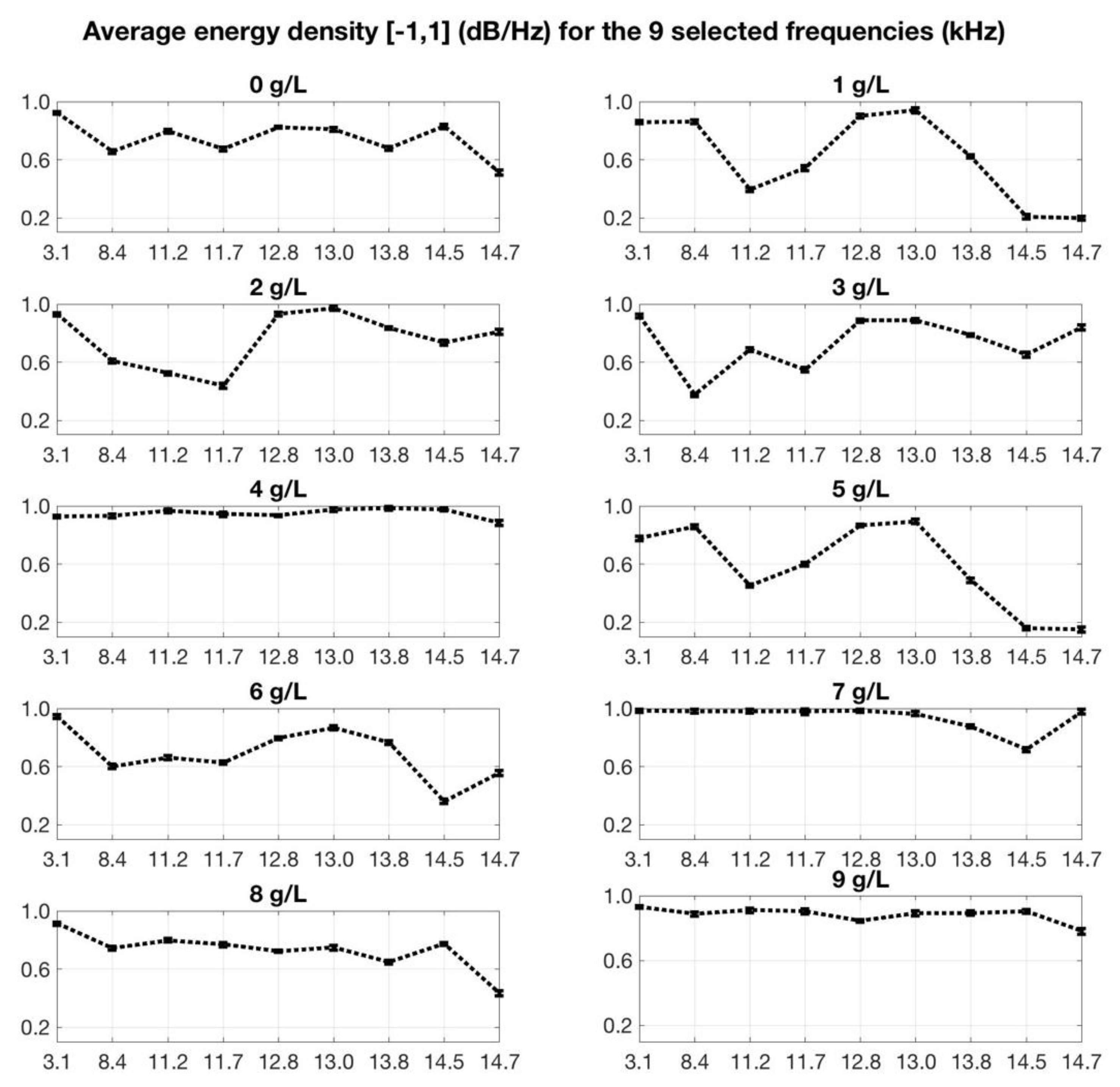
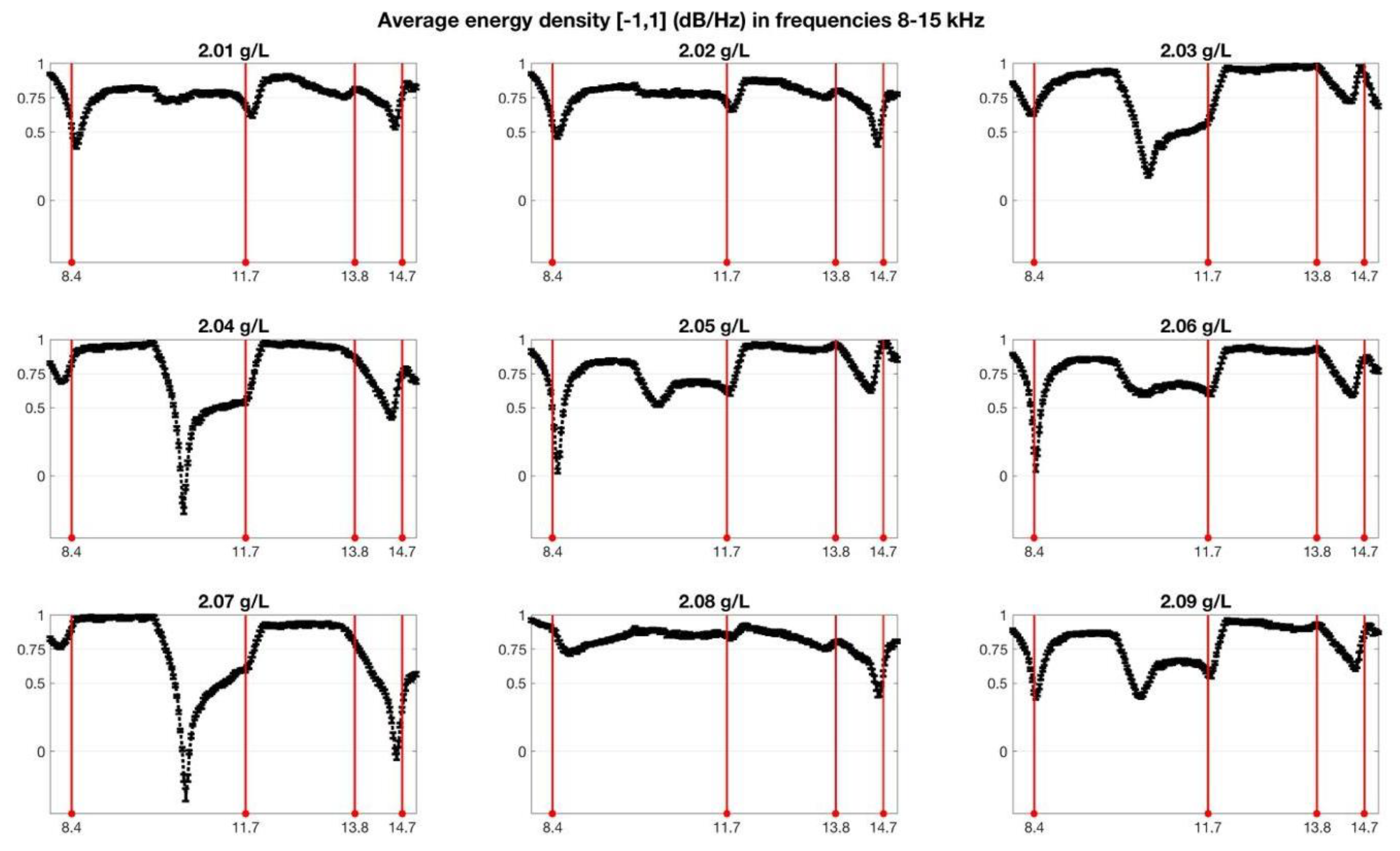
4.2. Feature Extraction

The GGA+ELM algorithm performs feature extraction optimizing the accuracy classification of samples according to their fructose concentration. The genetic algorithm is fed with spectral information as shown in Figure 4. Each feature is a spectral line. The optimal solution, if it exists, is unknown. The algorithm delivers two of the best solutions found in the execution. Each solution is composed of a set of frequencies (feature extraction) that classify with high accuracy. Not all solutions have the same number of frequencies.

A 2.7 GHz Intel Core i7 processor was used. The specific parameter values of the GGA and ELM are summarized below. Five independent simulations were performed for each of the three sets of samples. The time for each simulation was approximately 1 h, so the total computation time was about 15 h.

• Maximum number of generations = 50 generations;
• Training data size = 80%;
• Testing data size = 20%;
• Population size = 50 individuals;
• Mutation probability = 0.1;
• Number of neurons of ELM = 10 in Table 1; ELM = 11 in Table 2 and Table 3.

No information on which frequencies to be tested first was given to the algorithm.

Table 4. Characteristics of the two classifiers provided by GGA+ELM to discriminate the fructose concentrations of Table 1, Table 2 and Table 3. The classifiers make a decision according to the value of aver-age energy density on specific frequencies in the acoustic response spectrum.

Frequencies (kHz)	Classifier 1	Classifier 2
f1	8.4	3.1
f2	11.7	11.2
f3	13.8	12.8
f4	14.7	13.0
f5	-	14.5

lists the frequencies (kHz) of the independent classifiers. Classifier 1 consists of 4 frequencies in the range (8–15) kHz, and Classifier 2 selects five frequencies in the range (3–15]) kHz. The two classifiers are combined into a single classification system. It is note-worthy that with only nine features can characterize the 28 concentrations in Table 1, Table 2 and Table 3.

4.3. Discussion

A total of 20 M random and independent iterations was run for the two independent classifiers and the combined classifier on random test sets. The results are reported in

Table 5. Performance of the two classifiers provided by GGA+ELM and the voting system classifier to discriminate the fructose concentrations referred in Table 1, Table 2 and Table 3. The average values and standard deviation of the accuracy were estimated from 20 M independent and random iterations.

Classifier	0–9 g/L (±1 g/L)		2.0–3.0 g/L (±0.1 g/L)		2.00–2.10 g/L (±0.01 g/L)
	Average Accuracy	Standard Deviation	Average Accuracy	Standard Deviation	Average Accuracy	Standard Deviation
1	99.71	0.0126	90.32	0.0704	98.65	0.0272
2	97.60	0.0415	85.89	0.0727	80.78	0.0824
Combined classifier	99.82	0.0123	98.98	0.0266	98.65	0.0272

. For each set of concentrations (±1 g/L, ±0.1 g/L, and ±0.01 g/L) the average value and standard deviation of the classification accuracy are given.

Overall, it is observed that the combined classifier is valid for all concentrations in Table 1, Table 2 and Table 3 (with a minimum average accuracy of 98.65% over the 20 M iterations). As the average classification accuracy decreases, the difference between sample concentrations b becomes smaller: 99.82% at ±1 g/L (Table 1), 98.98% at ±0.1 g/L (Table 2), and 98.65% at ±0.01 g/L (Table 3). The standard deviation also increases in this direction: 0.0123 with ±1 g/L (Table 1), 0.0266 with ±0.1 g/L (Table 2), and 0.0272 with ±0.01 g/L (Table 3). This pattern meets the expected results: the difficulty of discrimination rises with higher class similarity. In the following lines, we elaborate on the results for each set of classes (fructose concentration), analyzing Table 1, Table 2 and Table 3 separately.

The classification of the samples of Table 1 (0–9 g/L) has very satisfactory results with the three classifiers: Classifier 1 and 2 of Table 4 and the combined classifier of them. With the three classifiers an average accuracy of more than 97% over 20 M random iterations is obtained. It is very remarkable that Classifier 1 can characterize, with only four spectral lines, up to ten concentrations with an average accuracy of 99.71%. Combining the two decision-makers in a single classifier achieves an average accuracy of better than 99.8%.

The nine frequencies of the combined classifier are located in the range (3–15) kHz. These frequencies have been highlighted in Figure 5 on the spectral information of the vibrational absorption bands for each concentration of Table 1. Note that the combination of these spectral lines allows the ten classes to be differentiated. Not all frequencies are equally important in the classification operation, some frequencies are more decisive in the classification among several classes. There may be other sets of frequencies that classify the samples with similar accuracy. The optimization algorithm offers solutions close to the optimal solution, without ensuring that there is a unique solution.

Figure 6 shows ten different patterns for the concentration classification of Table 1. Each pattern is constructed with the average normalized energy density value for each of the nine frequencies at a concentration from Table 1. The similarity between some patterns is interesting. For example, the curve characterizing the 1 g/L concentration is similar to the 5 g/L concentration pattern. The same happens with the 4 g/L and 9 g/L concentration patterns. This phenomenon has been reproduced in all the experiments performed and we believe that it may be associated with the resonance of the container used.

The application of the combined classifier on 143 samples from Table 2 (concentrations between 2.0 g/L and 3.0 g/L with increments of ±0.1 g/L) provided satisfactory results. As in the previous case, a sequence of 20M random and independent iterations was carried out. As shown in Table 5, Classifiers 1 and 2 obtained an average accuracy higher than 85%, whereas their combined classifier improves the average classification accuracy to 98.98% with a standard deviation 0.0266. This result is very satisfactory, although worse than that obtained for 1 g/L concentrations. The greater the similarity among classes, the more complex the classification and the lower the precision.

Figure 7 presents the patterns for the concentrations between 2.1 g/L and 2.9 g/L. These have been generated from the average and normalized energy density values for the nine frequencies of the combined classifier. Very similar values are observed in general since the variation in concentration is only ±0.1 g/L. Extreme closeness is appreciated in some cases such as the 2.3 g/L and 2.4 g/L concentrations, also with the 2.8 g/L and 2.9 g/L concentrations.

For classes with a concentration difference of ±0.01 g/L in Table 3, the 143 samples were also analyzed by Classifiers 1, 2 and the combined system. The last columns of Table 5 show the results obtained by each classifier over 20M random and independent iterations. Classifier 1, with 4 frequencies in the 8–15 kHz range and an average classification accuracy of 98.65% was much more effective than Classifier 2, where the accuracy de-creased to 80.78%. The combination of both classifiers did not improve the accuracy of Classifier 1, so the combined system considers only the decision of the first classifier, ignoring the decision of the second one. As discussed in the beginning of the section for the concentrations of Table 1, not all frequencies contribute equally in the classification. At the high similarity concentrations of Table 3, the frequencies of Classifier 2 do not add new information in the decision process over the information of Classifier 1. As a result, all the samples were classified with an average accuracy of 98.65% and a standard deviation of 0.0272.

The allocation of the four frequencies of Classifier 1 in the middle band of the spectrum, between 8 and 15 kHz, is understandable. It is the band with high mean energy density values. Figure 8 shows the position of these frequencies in the mean spectra of the nine concentrations between 2.01 g/L and 2.09 g/L. Figure 9 shows the patterns generated by Classifier 1 of the average and normalized energy density for the four frequencies. As in the previous cases there are very similar patterns, for example in the 2.01 g/L and 2.02 g/L patterns. There is also close similarity between the 2.03 g/L, 2.05 g/L, and 2.09 g/L patterns.

5. Conclusions

We have described a new non-invasive method based on the spectral analysis of audible scattered sounds to conclude the concentration of liquid mixtures according to their chemical composition with low cost. The spectral information was analyzed by a metaheuristic algorithm. ELM was integrated to implement the fitness function of the optimization algorithm GGA and extract a reduced set of frequencies as a classifier. The acoustical response spectrum of the samples to MLS sounds was used after a previous comparison with other sounds, like chirps, square pulses, and white noise. It was sufficient to examine the spectrum response at a few frequencies instead of analyzing the whole range of audible frequencies.

The experiments were carried out with 364 measurements from 28 samples of distilled water and fructose mixtures (150 mL) with a fructose concentration varying between 0 and 9 g/L. The 28 concentrations were grouped into three sets with increasing difficulty: ten between concentrations 0 g/L and 9 g/L with ±1 g/L increments, nine concentrations between 2.1 g/L and 2.9 g/L with ±0.1 g/L increments, and nine between 2.01 g/L and 2.09 g/L with ±0.01 g/L increments.

This work has allowed us to reduce the problem to a set of only nine frequencies on (3–15) kHz able to classify samples with concentrations of any of the three sets described. In the most complex case, the proposed classifier was able to discriminate fructose concentrations with variations of ±0.01 g/L with an average accuracy of 98.65%. The higher the concentration difference, the better the classification accuracy. For samples with increments of ±0.1 g/L the average accuracy is 98.98%, and when the concentration increments are ±1 g/L, the average accuracy rises to 99.82%.

The optimization algorithm returned different solutions with similar performance. The solution to the problem was not unique. It is important to note that changes in the number of types are likely to change the set of frequencies selected in the solutions. Each frequency had a different weight in the classification process. Future research will be focused on analyzing other chemicals, more complex mixtures and improving the accuracy of this sensing method.

References

1. Bonacucina, G.; Cespi, M.; Mencarelli, G.; Casettari, L.; Palmieri, G.F. The Use of Acoustic Spectroscopy in the Characterisation of Ternary Phase Diagrams. Int. J. Pharm. 2013, 441, 603–610. [Google Scholar] [CrossRef]
2. Bonacucina, G.; Perinelli, D.R.; Cespi, M.; Casettari, L.; Cossi, R.; Blasi, P.; Palmieri, G.F. Acoustic Spectroscopy: A Powerful Analytical Method for The Pharmaceutical Field? Int. J. Pharm. 2016, 503, 174–195. [Google Scholar] [CrossRef] [PubMed]
3. Dukhin, A.S.; Goetz, P.J. Ultrasound for Characterizing Colloids. In ACS Symposium Series; American Chemical Society: Washington, DC, USA, 1999, 2004; pp. 91–120. [Google Scholar]
4. Povey, M.J. Ultrasonic Techniques for Fluids Characterization; Elsevier: Amsterdam, The Netherlands, 1997. [Google Scholar]
5. Contreras, N.I.; Fairley, P.; McClements, D.J.; Povey, M.J. Analysis of The Sugar Content of Fruit Juices and Drinks Using Ultrasonic Velocity Measurements. Int. J. Food Sci. Technol. 1992, 27, 515–529. [Google Scholar] [CrossRef]
6. Dzida, M.; Zorebski, E.; Zorębski, M.; Żarska, M.; Geppert-Rybczyńska, M.; Chorążewski, M.; Cibulka, I. Speed of Sound and Ultrasound Absorption in Ionic Liquids. Chem. Rev. 2017, 117, 3883–3929. [Google Scholar] [CrossRef] [Green Version]
7. Santos, J.; Ferreira, A.; Santos, M.; Vasco, J.; Cardoso, M.; Ramalho, A. Versatile Low Cost Device for Measuring The Sound Speed in Liquids. In Proceedings of the Meetings on Acoustics ICU, Bruges, Belgium, 3–6 September 2019. [Google Scholar]
8. Dukhin, A.S.; Goetz, P.J. Acoustic and Electroacoustic Spectroscopy for Characterizing Concentrated Dispersions and Emulsions. Adv. Colloid Interface Sci. 2001, 92, 73–132. [Google Scholar] [CrossRef]
9. Habrioux, M.; Nasri, D.; Daridon, J.L. Measurement of Speed of Sound, Density Compressibility and Viscosity in Liquid Methyl Laurate and Ethyl Laurate up to 200 MPa by Using Acoustic Wave Sensors. J. Chem. Thermodyn. 2018, 120, 1–12. [Google Scholar] [CrossRef]
10. Javed, M.A.; Baumhögger, E.; Vrabec, J. Thermodynamic Speed of Sound Data for Liquid and Supercritical Alcohols. J. Chem. Eng. Data 2019, 64, 1035–1044. [Google Scholar] [CrossRef] [Green Version]
11. Holmes, M.J.; Parker, N.G.; Povey, M.J.W. Temperature Dependence of Bulk Viscosity in Water Using Acoustic Spectroscopy. In Journal of Physics: Conference Series; IOP Publishing: Bristol, UK, 2011; Volume 269, No. 1; p. 012011. [Google Scholar]
12. Hoche, S.; Hussein, M.A.; Becker, T. Density, Ultrasound Velocity, Acoustic Impedance, Reflection and Absorption Coefficient Determination of Liquids via Multiple Reflection Method. Ultrasonics 2015, 57, 65–71. [Google Scholar] [CrossRef]
13. Pal, B.; Roy, S. Probing Aqueous Electrolytes with Fourier Spectrum Pulse-Echo Technique. J. Mol. Liq. 2019, 291, 111302. [Google Scholar] [CrossRef] [Green Version]
14. Pal, B. Fourier Spectrum Pulse-Echo for Acoustic Characterization. J. Nondestruct. Eval. 2018, 37, 1–4. [Google Scholar] [CrossRef] [Green Version]
15. Povey, M.J. Ultrasound Particle Sizing: A Review. Particuology 2013, 11, 135–147. [Google Scholar] [CrossRef]
16. Silva, C.A.; Saraiva, S.V.; Bonetti, D.; Higuti, R.T.; Cunha, R.L.; Pereira, L.O.; Fileti, A.M. Application of Acoustic Models for Polydisperse Emulsion Characterization using Ultrasonic Spectroscopy in The Long Wavelength Regime. Colloids Surf. A Physicochem. Eng. Asp. 2020, 602, 125062. [Google Scholar] [CrossRef]
17. Vos, B.; Crowley, S.V.; O’Sullivan, J.; Evans-Hurson, R.; McSweeney, S.; Krüse, J.; O’mahony, J.A. New Insights into the Mechanism of Rehydration of Milk Protein Concentrate Powders Determined by Broadband Acoustic Resonance Dissolution Spectroscopy (BARDS). Food Hydrocoll. 2016, 61, 933–945. [Google Scholar] [CrossRef] [Green Version]
18. Yan, J.; Wright, W.M.; O’Mahony, J.A.; Roos, Y.; Cuijpers, E.; van Ruth, S.M. A Sound Approach: Exploring a Rapid and Non-Destructive Ultrasonic Pulse Echo System for Vegetable Oils Characterization. Food Res. Int. 2019, 125, 108552. [Google Scholar] [CrossRef]
19. Buckin, V. High-Resolution Ultrasonic Spectroscopy. J. Sens. Sens. Syst. 2018, 7, 207–217. [Google Scholar] [CrossRef]
20. Page, J.H. Ultrasonic Spectroscopy of Complex Media. Nano Optics and Atomics: Transport of Light and Matter Waves. In Proceedings of the International School of Physics “Enrico Fermi”, Course CLXXIII, Varenna, Italy, 23 June–3 July 2011; pp. 115–131. [Google Scholar]
21. Buckin, V.; Altas, M.C. Ultrasonic Monitoring of Biocatalysis in Solutions and Complex Dispersions. Catalysts 2017, 7, 336. [Google Scholar] [CrossRef] [Green Version]
22. Murdoch, N.; Chide, B.; Lasue, J.; Cadu, A.; Sournac, A.; Bassas-Portús, M.; Mimoun, D. Laser-Induced Breakdown Spectroscopy Acoustic Testing of the Mars 2020 Microphone. Planet. Space Sci. 2019, 165, 260–271. [Google Scholar] [CrossRef] [Green Version]
23. Chide, B.; Maurice, S.; Murdoch, N.; Lasue, J.; Bousquet, B.; Jacob, X.; Wiens, R.C. Listening to Laser Sparks: A Link between Laser-Induced Breakdown Spectroscopy, Acoustic Measurements and Crater Morphology. Spectrochim. Acta Part B At. Spectrosc. 2019, 153, 50–60. [Google Scholar] [CrossRef] [Green Version]
24. Jahanshahi, A.; Sabzi, H.Z.; Lau, C.; Wong, D. GPU-NEST: Characterizing Energy Efficiency of Multi-GPU Inference Servers. IEEE Comput. Archit. Lett. 2020, 19, 139–142. [Google Scholar] [CrossRef]
25. Jahanshahi, A. Tinycnn: A Tiny Modular CNN Accelerator for Embedded FPGA. arXiv 2019, arXiv:1911.06777. [Google Scholar]
26. Wu, C.; Shao, S.; Tunc, C.; Hariri, S. Video Anomaly Detection Using Pre-Trained Deep Convolutional Neural Nets and Context Mining. In Proceedings of the 2020 IEEE/ACS 17th International Conference on Computer Systems and Applications (AICCSA), Antalya, Turkey, 2–5 November 2020; pp. 1–8. [Google Scholar]
27. Khan, S.; Rahmani, H.; Shah, S.A.A.; Bennamoun, M.A. Guide to Convolutional Neural Networks for Computer Vision. Synth. Lect. Comput. Vis. 2018, 8, 1–207. [Google Scholar] [CrossRef]
28. Luo, X.J.; Oyedele, L.O.; Ajayi, A.O.; Akinade, O.O.; Owolabi, H.A.; Ahmed, A. Feature Extraction and Genetic Algorithm Enhanced Adaptive Deep Neural Network for Energy Consumption Prediction in Buildings. Renew. Sustain. Energy Rev. 2020, 131, 109980. [Google Scholar] [CrossRef]
29. Tran, D.H.; Luong, D.L.; Chou, J.S. Nature-Inspired Metaheuristic Ensemble Model for Forecasting Energy Consumption in Residential Buildings. Energy 2020, 191, 116552. [Google Scholar] [CrossRef]
30. Roshani, M.; Phan, G.T.; Ali, P.J.M.; Roshani, G.H.; Hanus, R.; Duong, T.; Kalmoun, E.M. Evaluation of Flow Pattern Recognition and Void Fraction Measurement in Two Phase Flow Independent of Oil Pipeline’s Scale Layer Thickness. Alex. Eng. J. 2021, 60, 1955–1966. [Google Scholar] [CrossRef]
31. Nabavi, M.; Elveny, M.; Danshina, S.D.; Behroyan, I.; Babanezhad, M. Velocity prediction of Cu/Water Nanofluid Convective Flow in a Circular Tube: Learning CFD data by Differential Evolution Algorithm Based Fuzzy Inference System (DEFIS). Int. Commun. Heat Mass Transf. 2021, 126, 105373. [Google Scholar] [CrossRef]
32. Roshani, M.; Sattari, M.A.; Ali, P.J.M.; Roshani, G.H.; Nazemi, B.; Corniani, E.; Nazemi, E. Application of GMDH Neural Network Technique to Improve Measuring Precision of a Simplified Photon Attenuation based Two-Phase Flowmeter. Flow Meas. Instrum. 2020, 75, 101804. [Google Scholar] [CrossRef]
33. Hong, T.; Pinson, P.; Wang, Y.; Weron, R.; Yang, D.; Zareipour, H. Energy Forecasting: A review and Outlook. IEEE Open Access J. Power Energy 2020. [Google Scholar] [CrossRef]
34. Runge, J.; Zmeureanu, R. Forecasting Energy Use in Buildings Using Artificial Neural Networks: A Review. Energies 2019, 12, 3254. [Google Scholar] [CrossRef] [Green Version]
35. Mason, K.; Duggan, J.; Howley, E. Forecasting Energy Demand, Wind Generation and Carbon Dioxide Emissions in Ireland using Evolutionary Neural Networks. Energy 2018, 155, 705–720. [Google Scholar] [CrossRef]
36. Arabi, M.; Dehshiri, A.M.; Shokrgozar, M. Modeling Transportation Supply and Demand Forecasting using Artificial Intelligence Parameters (Bayesian model). J. Appl. Eng. Sci. 2018, 16, 43–49. [Google Scholar] [CrossRef] [Green Version]
37. Li, Y.; Chen, X.; Yu, J. A Hybrid Energy Feature Extraction Approach for Ship-Radiated Noise based on CEEMDAN Combined with Energy Difference and Energy Entropy. Processes 2019, 7, 69. [Google Scholar] [CrossRef] [Green Version]
38. García Díaz, P.; Martínez Rojas, J.A.; Utrilla Manso, M.; Monasterio Expósito, L. Analysis of Water, Ethanol, and Fructose Mixtures using Nondestructive Resonant Spectroscopy of Mechanical Vibrations and a Grouping Genetic Algorithm. Sensors 2018, 18, 2695. [Google Scholar] [CrossRef] [PubMed] [Green Version]
39. Praat: Doing Phonetics by Computer. Available online: http://www.praat.org/ (accessed on 1 June 2021).
40. Audacity ® | Free, Open Source, Cross-Platform Audio Software. Available online: https://www.audacityteam.org (accessed on 1 June 2021).
41. MATLAB for Artificial Intelligence. Available online: https://www.mathworks.com/ (accessed on 1 June 2021).
42. García-Díaz, P.; Sánchez-Berriel, I.; Martínez-Rojas, J.A.; Diez-Pascual, A.M. Unsupervised Feature Selection Algorithm for Multiclass Cancer Classification of Gene Expression RNA-Seq Data. Genomics 2020, 112, 1916–1925. [Google Scholar] [CrossRef] [PubMed]
43. De Lit, P.; Falkenauer, E.; Delchambre, A. Grouping Genetic Algorithms: An Efficient Method to Solve the Cell Formation Problem. Math. Comput. Simul. 2000, 51, 257–271. [Google Scholar] [CrossRef]
44. Falkenauer, E. The Grouping Genetic Algorithms: Widening the Scope of the GAs. Belg. J. Oper. Research. Stat. Comput. Sci. 1993, 33, 79–102. [Google Scholar]
45. Falkenauer, E. Genetic Algorithms for Grouping Problems; Wiley: New York, NY, USA, 1998. [Google Scholar]
46. James, T.L.; Brown, E.C.; Keeling, K.B. A Hybrid Grouping Genetic Algorithm for the Cell Formation Problem. Comput. Oper. Res. 2007, 34, 2059–2079. [Google Scholar] [CrossRef]
47. Brown, E.C.; Sumichrast, R.T. Evaluating Performance Advantages of Grouping Genetic Algorithms. Eng. Appl. Artif. Intell. 2005, 18, 1–12. [Google Scholar] [CrossRef]
48. Huang, G.B.; Zhu, Q.Y. Extreme Learning Machine: Theory and Applications. Neurocomputing 2006, 70, 489–501. [Google Scholar] [CrossRef]
49. Huang, G.B.; Chen, L. Convex Incremental Extreme Learning Machine. Neurocomputing 2007, 70, 3056–3062. [Google Scholar] [CrossRef]
50. Huang, G.B.; Chen, L. Enhanced Random Search Based Incremental Extreme Learning Machine. Neurocomputing 2008, 71, 3460–3468. [Google Scholar] [CrossRef]
51. Huang, G.B.; Xiaojian, H.; Zhou, D. Optimization Method based Extreme Learning Machine for Classification. Neurocomputing 2010, 74, 155–163. [Google Scholar] [CrossRef]
52. Huang, G.B.; Wang, D.H.; Lan, Y. Extreme Learning Machines: A Survey. Int. J. Mach. Learn. Cybern. 2011, 2, 107–122. [Google Scholar] [CrossRef]
53. Huang, G.B.; Zhou, H.; Ding, X.; Zhang, R. Extreme Learning Machine for Regression and Multiclass Classification. IEEE Trans. Syst. Man Cybern. Part B Cybern. 2012, 42, 513–529. [Google Scholar] [CrossRef] [Green Version]
54. Luo, X.; Chang, X.; Ban, X. Regression and Classification using Extreme Learning Machine based on L1-Norm and L2-Norm. Neurocomputing 2016, 174, 179–186. [Google Scholar] [CrossRef]
55. Cornejo-Bueno, L.; Nieto-Borge, J.C.; García-Díaz, P.; Rodríguez, G.; Salcedo-Sanz, S. Significant Wave Height and Energy Flux Prediction for Marine Energy Applications: A Grouping Genetic Algorithm—Extreme Learning Machine Approach. Renew. Energy 2016, 97, 380–389. [Google Scholar] [CrossRef]
56. Duan, L.; Bao, M.; Miao, J.; Xu, Y.; Chen, J. Classification Based on Multilayer Extreme Learning Machine for Motor Imagery Task form EEG signals. Procedia Comput. Sci. 2016, 88, 176–184. [Google Scholar] [CrossRef] [Green Version]
57. Kohavi, R.l.; Jonh, G.H. Wrappers for Features Subset Selection. Artif. Intell. 1997, 97, 273–324. [Google Scholar] [CrossRef] [Green Version]
58. Yao, X.; Liu, Y.; Lin, G. Evolutionary Programming Made Faster. IEEE Trans. Evol. Comput. 1999, 3, 82–102. [Google Scholar]
59. Quiroz-Castellanos, M.; Cruz-Reyes, L.; Torres-Jimenez, J.; Gómez S., C.; Fraire Huacuja, H.J.; Alvim, A.C.F. A Grouping Genetic Algorithm with Controlled Gene Transmission for The Bin Packing Problem. Comput. Oper. Res. 2015, 55, 52–64. [Google Scholar] [CrossRef]
60. Wicker, D.; Rizki, M.M.; Tamburino, L.A. The Multi-Tiered Tournament Selection for Evolutionary Neural Network Synthesis, Symposium on Combinations of Evolutionary Computation and Neural Networks. IEEE 2000, 207–215. [Google Scholar]
61. Xie, H.; Zhang, M.; Andreae, P.; Johnson, M. An Analysis of Multi-Sampled Issue and No-Replacement Tournament Selection. In Proceedings of the 10th annual conference on Genetic and evolutionary computation, Atlanta, GA, USA, July 2008; pp. 1323–1330. [Google Scholar]
Figure 1. Photograph of the experimental installation.
Applsci 11 07301 g001
Figure 2. Frequency response of the anechoic chamber.
Applsci 11 07301 g002
Figure 3. Recording of the sound card without signal.
Applsci 11 07301 g003
Figure 4. Spectral information of the vibrational absorption bands of ten different concentrations of fructose in distilled water (from 0 g/L to 9 g/L). The curves represent average and normalized values of sound pressure level (dB/Hz) over the audible frequencies range (20 Hz–22.05 kHz) for the samples from Table 1.
Applsci 11 07301 g004aApplsci 11 07301 g004b
Figure 5. Spectral information of vibrational absorption bands of 10 concentrations from 0 g/L to 9 g/L. The curves represent the average and normalized values of the sound pressure level (dB/Hz) over the audible frequencies range. In each spectrum, the frequencies used for both classifiers are emphasized.
Applsci 11 07301 g005
Figure 6. Spectral information patterns for fructose concentrations from 0 g/L to 9 g/L, with the average and normalized value of the sound pressure level (dB/Hz) as a function of the frequencies (kHz) used by the combined classifier.
Applsci 11 07301 g006
Figure 7. Spectral information patterns for fructose concentrations from 2.1 g/L to 2.9, with the average and normalized value of the sound pressure level (dB/Hz) as a function of the frequencies (kHz) used by the combined classifier.
Applsci 11 07301 g007
Figure 8. Spectral information of vibrational absorption bands of ten concentrations from 0 g/L to 9 g/L. The curves represent the average and normalized values of the sound pressure level (dB/Hz) over the audible frequencies range. In each spectrum, the frequencies used for both classifiers are emphasized.
Applsci 11 07301 g008
Figure 9. Spectral information patterns for fructose concentrations from 2.01 g/L to 2.09, with the average and normalized value of the sound pressure level (dB/Hz) as a function of the frequencies (kHz) used by the classifier 1.
Applsci 11 07301 g009