Communication

Modelling the Effect of Temperature on the Initial Decline during the Lag Phase of Geotrichum candidum

by
Ľubomír Valík
,
Petra Šipošová
,
Martina Koňuchová
* and
Alžbeta Medveďová
Department of Nutrition and Food Quality Assessment, Faculty of Chemical and Food Technology, Institute of Food Science and Nutrition, Slovak University of Technology in Bratislava, Radlinského 9, SK-812 37 Bratislava, Slovakia
*
Author to whom correspondence should be addressed.
Appl. Sci. 2021, 11(16), 7344; https://doi.org/10.3390/app11167344
Submission received: 13 July 2021 / Revised: 4 August 2021 / Accepted: 7 August 2021 / Published: 10 August 2021

Abstract

:
The study of lag phase provides essential knowledge for food quality control. With respect to significance of Geotrichum candidum in the food context, the aim of this study was to quantitatively characterize the relationship between temperature (6–25 °C) and initial decline period during G. candidum lag phase. The decrease in G. candidum cells in the lag phase was primary modelled by Weibull’s model to define the first-decimal reduction time (δ). Subsequently, the lag death rate (LDR) values were recalculated from δ and further modelled by using Arrhenius equations, as well as a square root model, and the models’ suitability was proven by selected statistical indices. The square root model with the estimated parameters b = 0.016 °C−1 h−0.5 and Tmin = −0.72 °C showed better indices relating to goodness of fit based on a low root mean sum of square error (RMSE = 0.028 log CFU mL−1), a higher coefficient of determination (R2 = 0.978), and the lowest value of AIC (AIC = −38.65). The present study provides a solution to the possible application of secondary predictive models to the death rate dependence on temperature during the microbial lag phase. Despite limited practical importance, under specific conditions, it is possible to consider its use, for example, in exposure assessment.

1. Introduction

Geotrichum candidum Link:Fr. is a filamentous yeast-like fungus that is commonly found in foodstuffs and food processing environments. G. candidum is often characterized as an intermediate between molds and yeasts. Today, this microorganism is accepted as the yeast with mouldy tendencies by the major taxonomic monography of De Hoog et al. [1]. In culture, G. candidum produces expanding, white- to cream-coloured, flat colonies. Microscopic appearance of G. candidum shows septate branching hyphae, which disarticulate almost entirely into rectangular arthroconidia (5–6 × 5–17 µm). The predominant branching pattern exhibited by fungal hyphae is di- or trichotomous branching of the peripheral hyphae [1,2,3].
The significance of this yeast in food production may be considered from positive and negative aspects. G. candidum is commonly used as an adjunct culture for the production of many ripened cheeses (e.g., soft mould-ripened cheeses, soft and semi-hard smear-ripened cheeses, and acid-coagulated cheeses). This fungus positively affects appearance, texture, taste and aroma of cheeses, due to its metabolic activity [4,5,6]. On the other hand, G. candidum is also considered as a frequent spoilage organism [7,8,9,10]. If G. candidum is present in excessive quantities on the surface of raw soft-ripened cheeses, (camembert type), it is considered to be responsible for many defects, such as unstable or slippery rind and unequal covering of the cheese surface [7,8,11]. In addition, G. candidum can cause degradation of milk fat and protein which results in creating undesirable cheese organoleptic properties and appearance [6,10,12]. In terms of shelf life and the microbial quality of food products, detailed knowledge of G. candidum behaviour in food matrices is needed.
This ascomycetous yeast can grow in a wide range of environmental conditions, notably temperature and pH values. G. candidum can grow in the temperature range from 5 to 38 °C, but its optimum growth temperature is around 25–30 °C [7,10,13,14]. Although it remains active over a wide pH interval (pH 3.0–11.5), its growth is stimulated by an acidic environment (pH 5.0–5.5). Generally, this milk yeast is particularly sensitive to the salt content in a medium, however, this sensitivity is strain-dependent [12,13]. According to Uraz and Özer [13], 1.0% (w/v) of salt in the environment can slow its growth and, at 5–6% salt content in media, an inhibitory effect is observed.
Microbial growth in food usually exhibits three distinctive phases, including the lag, exponential, and stationary phases [15]. The first growth phase, the lag phase, is generally known as a transition period of non-replication, during which microorganisms adjust to the new environment [16,17,18]. This process includes changes in the physiological state of cells, the synthesis of cellular components, and the production of intermediate metabolites necessary for microbial growth. For spore-forming bacteria, the lag phase may also include germination and outgrowth of spores [15,19,20,21].
Graphically, the lag phase represents the time when a horizontal tangent to the growth curve at the log of the initial cell count intersects the linear extrapolation of the exponential phase [22,23,24]. Lag time is also explained in terms of the amount of work to be conducted by the microbial population to adjust to the new environment and the rate at which that work is performed [16,23,25]. Assuming that each population consists of subpopulations with different physiological states and growth rates oscillating around zero, the average of the total population rate should be close to or equal to zero before the exponential growth phase. In general, this idea was not only incorporated in differential equations used by Baranyi and Roberts [26] as starting points in their mechanistic growth model [27], but also accepted in other explanations of non-linear microbial responses, e.g., during inactivation or survival [28]. Yates and Smotzer [17] considered three microbial populations in their lag model, which was solved by a system of differential equations: a non-duplicating cell population that undergoes internal cellular changes, including osmoprotective processes; a second, non-duplicating population that is not able to adapt to the new environment; and a third, actively duplicating population. According to the authors, then, the course of the lag phase depended on the initial proportion of these subpopulations.
The lag phase, including the phenomenon of the decrease in viable microbe counts, has been known about for over a century and described with primary models; however, there is still a need for a better understanding of this phenomenon, since its course and duration are affected by many factors, including environmental factors [15,27,29]. Based on our observations, the decrease in G. candidum counts during the lag phase was observed, and it was affected by the incubation temperature. Therefore, the aim of this study was to model the effect of temperature on the decline rate of G. candidum in the early stages of the lag phase, in order to provide a deeper quantitative overview of the microbial growth phase, which is still highly variable.

2. Materials and Methods

2.1. Microorganism and Preparation of Inoculum

The G. candidum isolate J used in this study was obtained from traditional Slovak ripened curd cheese called Bryndza (Turčianske Teplice, Slovak Republic). Identification was performed on the basis of internal transcribed spacer (ITS) sequencing (additional details can be found in Pangallo et al. [30]). Phylogenetic analyses according to Groenewald et al. [31] revealed affinity of novel species to the Geotrichum candidum/Galactomyces candidus group. Molecular sequencing was confirmed by morphological and biochemical characteristics in accordance with Samson et al. [32] and De Hoog et al. [1].
The G. candidum isolate was maintained on slant skim milk agar (SMA, Merck, Darmstadt, Germany) and stored at 5 ± 0.5 °C. It was subcultured on horizontal SMA agar in tubes at 25 ± 0.5 °C for 72 h and, subsequently, two parallels of the isolate were mixed with 10 mL of sterile peptone–saline solution. The culture prepared in this way was appropriately diluted and used in the experiments with the inoculum level of approximately 102 CFU mL−1.
The strain was refrigerated (5 ± 1 °C) on plate count skim milk agar (SMA; Merck, Darmstadt, Germany) slants and periodically cultured in diluted SMA agar. For long-term storage, the cultures were frozen at −70 °C in tubes containing yeast malt broth (Sigma-Aldrich, St. Louis, MO, USA) supplemented with 20% glycerol.

2.2. Estimation of G. candidum Cell Viable Counts

Pre-tempered UHT milk with 1.5 g L−1 fat content (Rajo, Inc., Bratislava, Slovak Republic) with the addition of 1% NaCl (Centralchem Inc., Bratislava, Slovak Republic) was used in the experiments as cultivation medium for G. candidum growth. Three parallels of an inoculated milk medium were incubated at 8, 12, 15, 18, 21, and 25 ± 0.5 °C under static aerobic conditions. At 6 °C, three replicated cultivations in three parallels were performed due to an almost negligible decrease in G. candidum counts. The actual counts of viable G. candidum cells were determined at defined time intervals on DRBC agar (Biokar Diagnostics, Beauvais, France) in accordance with EN ISO 21527-1 [33] by a cultivation method using ten-fold dilution in a peptone–saline solution. Inoculated Petri dishes were cultivated in aerobic conditions at 25 ± 0.5 °C for 5 days.

2.3. Modelling of Lag Death Rate of G. candidum

Growth data of G. candidum in milk with 1% of NaCl addition were fitted with the DMfit model introduced by Baranyi and Roberts [27]. After repeatedly identifying decreases in the viable microbe counts (log CFU mL−1) at different incubation temperatures, the selected primary data from the lag phase were fitted with Weibull’s model Equation (1) as derived by Mafart et al. [34]:
l o g   N N 0 = ( t δ ) p
where N0 and N are the G. candidum cell viable counts (CFU mL−1) determined after inoculation and then during the lag phase in time t. The shape parameter p and the first decimal reduction δ (h) were estimated with non-linear regression performed with the Solver tool of Microsoft Excel 2013 (Microsoft, Redmond, WA, USA). δ, as the key output, was recalculated to the specific lag death rate LDR (kmax; h−1) according to Equation (2):
L D R = k max = ln 10 δ
It was then modelled as a function of temperature using the Arrhenius equation (Equation (3)). Then, according to Equation (4), it was reparametrized as per André et al. [35] and as modified by Davey [36]. Finally, the LDR was also modelled by the square root model (Equation (5); RTK) [37]:
ln k max = ln k * E a R · ( 1 T K 1 T K * )
ln k max = C 0 E a R · 1 T K
k max = b · ( T T min )
In Equations (3) and (4), kmax is the specific LDR (h−1) and k* is the death rate (h−1) at reference temperature TK*. Both TK* and incubation temperature TK are in K, Ea is the activation energy (kJ mol−1), R is the ideal gas constant (8.314.10−3 kJ mol−1 K−1), and C0 is the coefficient to be estimated by non-linear regression. For the square root model, b is the coefficient (°C−1 h−0.5), Tmin is the minimum temperature at which no decrease is expected, and T is the incubation temperature (°C).

2.4. Statistical Evaluation

The goodness of fit indices were evaluated by a calculation of the coefficient of determination (R2) according to Wells-Bennik et al. [38], with a root mean sum of square error (RMSE). Equation (6) characterized the experimental variability, and the variations between the observed values (yobs) and the fitted values (ypred) within the experiment with the replications.
R M S E = R S S D F = i = 1 n ( y i o b s y i p r e d ) 2 n n p
where RSS is the residual sum of square; DF is the degree of freedom; n is the number of observations; np is the number of parameters; and yi can include ln kmax or square root of kmax, dependent of the model equation used. For the variability between biologically independent reproductions (reproduction or biological variability), the same equations were used, although with a different number of observations. For example, there were three independent trials with two replicates (n = 46) and three parameters to be estimated at 6 °C.
Akaike’s Information Criterion (AIC) defined by Motulsky and Christopoulos [39] was used to compare the LDR temperature models as follows:
A I C = n · l n R S S n + 2 · ( p + 1 ) + 2 · ( p + 1 ) · ( p + 2 ) n p 2

3. Results and Discussion

3.1. Lag Death Rate Primary Modelling

The application of Weibull’s model to the lag phase data with the decrease in viable microbe counts in the temperature range of 6 to 12 °C is presented in Figure 1 and Supplementary Materials Figure S1. Despite the fact that the lag phase is considered the most variable microbial growth phase, it was obvious that a more intensive reduction in microbial cell viable counts was observed when the incubation temperature was higher. It was not only concerned with the increase in LDR; the process also began sooner, as the period of decrease in viable microbe counts was shorter with increased temperature. Finally, at 30 °C, the reduction was not observed at all (not presented here).
This resulted not only from the calculated model parameter δ but also from the relevant values of statistical indicators summarized in Table 1. A higher number of replicated observations at lower temperatures were mainly related with the experimental confirmation of a barely observable reduction in log CFU counts in the growth curve as a whole. This, however, enabled us to estimate the experimental variability as well as the biological variability of the observed phenomenon. The average RMSE values expressing the experimental variability in each independent trial, performed in duplicate, were 0.11 log CFU mL−1 and 0.13 log CFU mL−1 at 6 °C and 8 °C, respectively (data not included in Table 1), while the biological variability was represented with higher RMSE values of 0.200 log CFU mL−1 and 0.349 log CFU mL−1. The other values of RMSE in Table 1 represent only the biological variability that showed a maximum at 25 °C, the temperature at which the highest LDR or the lowest decimal reduction time of G. candidum was observed.

3.2. Lag Death Rate Secondary Modelling

Most of the phenomena associated with microbial adaptation mechanisms to new environmental conditions—involving the synthesis of cellular components, activation of genetic and metabolic processes, and accumulation of intracellular structures needed for cell division—are already known and well described. However, the lag phase is still considered poorly understood in the microbial growth [19]. At present, more than 120 years after the first mention in the literature of the lag phase, this may sound questionable; the lag kinetics have been described for individual cells [40], in different population levels, and even in the case when the microbial population declined [17]. However, the limited understanding of the lag phase is still true. To illustrate this fact, we did not find any mention of modelling the effect of environmental factors on the lag decline. In terms of suitable data for this research opportunity, we have only identified the addition of 1% NaCl in the case of G. candidum growth in milk. In this study, the lag phase data obtained from the growth curves observed in suboptimal temperatures growth range were fitted using Weibull´s model. Then, the LDR of G. candidum calculated from first decimal reductions δ (Table 1) was modelled using the secondary Arrhenius equations (Equations (3) and (4)) as well as with the square root model (Equation (5)). The calculated model parameters are summarized in Table 2. Both of the modified Arrhenius equations clearly demonstrated that the activation energy of 100.88 kJ mol−1 was needed for G. candidum arthrospores to germinate. In our case, they formed a substantial part of the inoculums (microscopic observation not presented in this study). The modified Arrhenius equations also provided the identical graphical outputs presented in Figure 2a, with a high coefficient of determination (R2 = 0.927). However, the application of the square root model presented in Figure 2b showed better indices relating to the goodness of fit involving RMSE (RMSE = 0.028 log CFU mL−1), a higher coefficient of determination (R2 = 0.978), and the lowest value of AIC value (Table 2).

4. Conclusions

The main message of this work was to show that, in some cases of the microbial lag phase, e.g., when the cell count decline is observed, the rate of death can depend on environmental factors. The application of secondary temperature models was demonstrated probably for the first time, and finally, associated with acceptable values of goodness of fit indices. The dependence of the lag phase decline on temperature will be still neglected in most cases. It is also worth noting that lag death rate modelling is possible. In special cases and when necessary, secondary modelling can be used; however, its practical relevance should be considered specifically from case to case. However, the gaps in the behaviour of microorganisms during the lag phase (e.g., in this study, from 20 h to 80 h within the range from 6 °C to 12 °C) may be relevant to uncertainty in microbial exposure assessment.

Supplementary Materials

The following are available online at https://www.mdpi.com/article/10.3390/app11167344/s1, Figure S1: Decrease in the cell numbers during lag phases of G. candidum growth in milk in the range of 15 °C to 25 °C.

Author Contributions

Conceptualization, Ľ.V., P.Š., A.M. and M.K.; methodology, Ľ.V.; validation, Ľ.V.; formal analysis, Ľ.V., P.Š. and A.M.; investigation, P.Š. and M.K.; resources, P.Š. and M.K.; writing—original draft preparation, Ľ.V. and P.Š.; writing—review and editing, A.M. and M.K.; visualization, Ľ.V.; supervision, Ľ.V.; project administration, Ľ.V. and A.M.; funding acquisition, Ľ.V. and A.M. All authors have read and agreed to the published version of the manuscript.

Funding

This research was funded by the Slovak Research and Development Agency, grant number APVV-19-0031 and the Scientific Grant Agency of the Ministry of Education, Science, Research and Sports of the Slovak Republic and Slovak Academy of Sciences, grant number VEGA 1/0532/18.

Institutional Review Board Statement

Not applicable.

Informed Consent Statement

Not applicable.

Data Availability Statement

The data presented in this study are available upon reasonable request from the corresponding author.

Conflicts of Interest

The authors declare no conflict of interest.

References

  1. De Hoog, G.S.; Guarro, J.; Gené, J.; Ahmed, S.A.; Al-Hatmi, A.M.S.; Figueras, M.J.; Vitale, R.G. Atlas of Clinical Fungi, The Ultimate Benchtool for Diagnostics, 4th ed.; Centraalbureau voor Schimmelcultures: Utrecht, The Netherlands, 2020; pp. 457–459. [Google Scholar]
  2. Kurtzman, C.P.; Fell, J.W.; Boekhout, T. The Yeasts: A Taxonomic Study; Elsevier: Amsterdam, The Netherlands, 2011. [Google Scholar]
  3. Thomidis, T.; Prodromou, I.; Farmakis, A.; Zambounis, A. Effect of temperature on the growth of Geotrichum candidum and chemical control of sour rot on tomatoes. Trop. Plant. Pathol. 2021. [Google Scholar] [CrossRef]
  4. Fröhlich-Wyder, M.T.; Arias-Roth, E.; Jakob, E. Cheese yeasts. Yeast 2018, 36, 129–141. [Google Scholar] [CrossRef] [PubMed]
  5. Jaster, H.; Judacewski, P.; Ribeiro, J.C.B.; Zielinski, A.A.F.; Demiate, I.M.; Los, P.R.; Alberti, A.; Nogueira, A. Quality assessment of the manufacture of new ripened soft cheese by Geotrichum candidum: Physicochemical and technological properties. Food Sci. Technol. 2019, 39, 50–58. [Google Scholar] [CrossRef] [Green Version]
  6. Šipošová, P.; Koňuchová, M.; Valík, Ľ.; Medveďová, A. Growth dynamics of lactic acid bacteria and dairy microscopic fungus Geotrichum candidum during their co-cultivation in milk. Food Sci. Technol. Int. 2020, in press. [Google Scholar] [CrossRef]
  7. Boutrou, R.; Guéguen, M. Interests in Geotrichum candidum for cheese technology. Int. J. Food Microbiol. 2005, 102, 1–20. [Google Scholar] [CrossRef]
  8. Garnier, L.; Valence, F.; Mounier, J. Diversity and control of spoilage fungi in dairy products: An update. Microorganisms 2017, 5, 42. [Google Scholar] [CrossRef] [PubMed] [Green Version]
  9. Eliskases-Lechner, F.; Guéguen, M.; Panoff, J.M. Geotrichum candidum. In Encyclopedia of Dairy Sciences, 2nd ed.; Fuquay, J.W., Fox, P.F., McSweeney, P.L.H., Eds.; Academic Press: London, UK, 2011; pp. 765–771. [Google Scholar]
  10. Koňuchová, M.; Valík, Ľ. Modelling the radial growth of Geotrichum candidum: Effects of temperature and water activity. Microorganisms 2021, 9, 532. [Google Scholar] [CrossRef] [PubMed]
  11. Laurenčík, M.; Sulo, P.; Sláviková, E.; Piecková, E.; Seman, M.; Ebringer, L. The diversity of eukaryotic microbiota in the traditional Slovak sheep cheese—Bryndza. Int. J. Food Microbiol. 2008, 127, 176–179. [Google Scholar] [CrossRef]
  12. Marcellino, N.; Benson, D.R. The good, the bad, and the ugly: Tales of mold-ripened cheese. Microbiol. Spectr. 2013, 1, 1–27. [Google Scholar] [CrossRef] [Green Version]
  13. Uraz, T.; Özer, B.H. Molds employed in food processing. In Encyclopedia of Food Microbiology, 2nd ed.; Batt, C.A., Tortello, M.-R., Eds.; Academic Press: Cambridge, UK, 2014; pp. 522–528. [Google Scholar]
  14. Šipošová, P.; Koňuchová, M.; Valík, Ľ.; Trebichavská, M.; Medveďová, A. Quantitative characterization of Geotrichum candidum growth in milk. Appl. Sci. 2021, 11, 4619. [Google Scholar] [CrossRef]
  15. Huang, L. Simulation and evaluation of different statistical functions for describing lag time distributions of bacterial growth curve. Microb. Risk Anal. 2016, 1, 47–55. [Google Scholar] [CrossRef]
  16. Robinson, T.P.; Ocio, M.J.; Kaloti, A.; Mackey, B.M. The effect of the growth environment on the lag phase of Listeria monocytogenes. Int. J. Food Microbiol. 1998, 44, 83–92. [Google Scholar] [CrossRef]
  17. Yates, G.T.; Smotzer, T. On the lag phase and initial decline of microbial growth curves. J. Theor. Biol. 2007, 244, 511–517. [Google Scholar] [CrossRef]
  18. Bertrand, R.L. Lag phase is a dynamic, organized, adaptive, and evolvable period that prepares bacteria for cell division. J. Bacteriol. 2019, 201, e00697-18. [Google Scholar] [CrossRef] [PubMed]
  19. Rolfe, M.D.; Rice, C.J.; Lucchini, S.; Pin, C.; Thompson, A.; Cameron, A.D.; Alston, M.; Stringer, M.F.; Betts, R.P.; Baranyi, J.; et al. Lag phase is a distinct growth phase that prepares bacteria for exponential growth and involves transient metal accumulation. J. Bacteriol. 2012, 194, 686–701. [Google Scholar] [CrossRef] [PubMed] [Green Version]
  20. Valík, Ľ.; Ačai, P. Predictive Microbiology and Microbiological Risk Assessment, 1st ed.; SUT: Bratislava, Slovakia, 2016; pp. 18–141. [Google Scholar]
  21. Hamill, P.; Stevenson, A.; McMullan, P.; Williams, J.; Lewis, A.; Sudharsan, S.; Stevenson, K.E.; Farnsworth, K.D.; Khroustalyova, G.; Takemoto, J.Y.; et al. Microbial lag phase can be indicative of, or independent from, cellular stress. Sci. Rep. 2020, 10, 1–20. [Google Scholar] [CrossRef]
  22. Baty, F.; Delignette-Muller, M.-L. Estimating the bacterial lag time: Which model, which precision? Int. J. Food Microbiol. 2004, 91, 261–277. [Google Scholar] [CrossRef] [PubMed]
  23. Swinnen, I.A.; Bernaerts, K.; Dens, E.J.; Geeraerd, A.H.; Van Impe, J.F. Predictive modelling of the microbial lag phase: A review. Int. J. Food Microbiol. 2004, 94, 137–159. [Google Scholar] [CrossRef]
  24. Métris, A.; Le Marc, Y.; Elfwing, A.; Ballagi, A.; Baranyi, J. Modelling the variability of lag times and the first generation times of single cells of E. Coli. Int. J. Food Microbiol. 2005, 100, 13–19. [Google Scholar] [CrossRef] [PubMed]
  25. Mellefont, L.A.; Ross, T. The effect of abrupt shifts in temperature on the lag phase duration of Escherichia coli and Klebsiella oxytoca. Int. J. Food Microbiol. 2003, 83, 295–305. [Google Scholar] [CrossRef]
  26. Baranyi, J.; Roberts, T.A. Mathematics of predictive food microbiology. Int. J. Food Microbiol. 1995, 26, 199–218. [Google Scholar] [CrossRef] [Green Version]
  27. Baranyi, J.; Roberts, T.A. A dynamic approach to predicting bacterial growth in food. Int. J. Food Microbiol. 1994, 23, 277–294. [Google Scholar] [CrossRef]
  28. Geeraerd, A.H.; Valdramidis, V.P.; Van Impe, J.F. GInaFiT, a freeware tool to assess non-log-linear microbial survivor curves. Int. J. Food Microbiol. 2005, 102, 95–105. [Google Scholar] [CrossRef] [PubMed]
  29. Schultz, D.; Kishony, R. Optimization and control in bacterial Lag phase. BMC Biol. 2013, 11, 120. [Google Scholar] [CrossRef] [Green Version]
  30. Pangallo, D.; Šaková, N.; Koreňová, J.; Puškárová, A.; Kraková, L.; Valík, Ľ.; Kuchta, T. Microbial diversity and dynamics during the production of May bryndza cheese. Int. J. Food Microbiol. 2014, 170, 38–43. [Google Scholar] [CrossRef] [PubMed]
  31. Groenewald, M.; Coutinho, T.; Smith, M.T.; van der Walt, J.P. Species reassignment of Geotrichum bryndzae, Geotrichum phurueaensis, Geotrichum silvicola, and Geotrichum vulgarae based on phylogenetic analyses and mating compatibility. Int. J. Syst. Evol. Microbiol. 2012, 62, 3072–3080. [Google Scholar] [CrossRef] [PubMed]
  32. Samson, R.A.; Hoekstra, E.S.; Frisvad, J.S.; Filtenborg, O. Introduction to Food and Airborne Fungi, 6th ed.; Centraalbureau voor Schimmelcultures: Utrecht, The Netherlands, 2002; pp. 28–389. [Google Scholar]
  33. ISO 21527-1:2008. Part 1: Colony count technique in products with water activity greater than 0.95. In Microbiology of Food and Animal Feeding Stuffs—Horizontal Method for the Enumeration of Yeasts and Molds; International Organization for Standardization: Geneva, Switzerland, 2010; pp. 1–12. [Google Scholar]
  34. Mafart, P.; Couvert, O.; Gaillard, S.; Leguerinel, I. On calculating sterility in thermal preservation methods: Application of the Weibull frequency distribution model. Int. J. Food Microbiol. 2002, 72, 107–113. [Google Scholar] [CrossRef] [Green Version]
  35. André, S.; Leguerinel, I.; Palop, A.; Desriac, N.; Planchon, S.; Mafart, P. Convergence of Bigelow and Arrhenius models over a wide range of heating temperatures. Int. J. Food Microbiol. 2019, 291, 173–180. [Google Scholar] [CrossRef] [PubMed]
  36. Davey, K.R. A predictive model for combined temperature and water activity on microbial growth during the growth phase. J. Appl. Bacteriol. 1989, 67, 483–488. [Google Scholar] [CrossRef]
  37. Ratkowsky, D.A.; Olley, J.; McMeekin, T.A.; Ball, A. Relationship between temperature and growth rate of bacterial cultures. J. Bacteriol. 1982, 149, 1–5. [Google Scholar] [CrossRef] [Green Version]
  38. Wells-Bennik, M.H.; Jansen, P.W.; Klaus, V.; Yang, C.; Zwietering, M.H.; den Besten, H.M. Heat resistance of spores of 18 strains of Geobacillus stearothermophilus and impact of culturing conditions. Int. J. Food Microbiol. 2019, 291, 161–172. [Google Scholar] [CrossRef] [PubMed]
  39. Motulsky, H.J.; Christopoulos, A. Fitting Models to Biological Data Using Linear and Nonlinear Regression. A practical Guide to Curve Fitting, 1st ed.; GraphPad Software: San Diego, CA, USA, 2003; pp. 13–346. [Google Scholar]
  40. Baranyi, J. Stochastic modelling of bacterial lag phase. Int. J. Food Microbiol. 2002, 73, 203–206. [Google Scholar] [CrossRef]
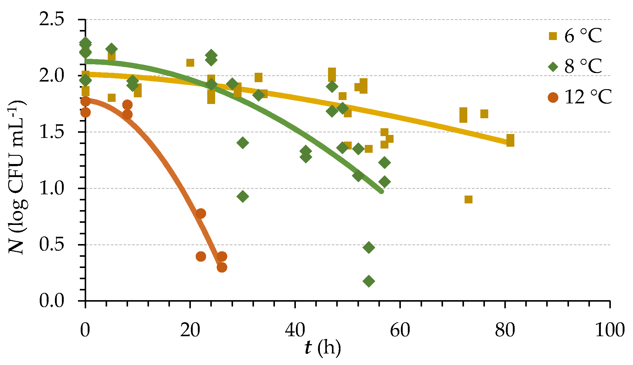
Figure 1. Decrease in the cell numbers during the lag phases of G. candidum growth in milk, in the range of 6 °C to 12 °C.
Applsci 11 07344 g001
Figure 2. Temperature dependence of G. candidum LDR modelled with the modified ARH models, identical for both equations (a). Graphical presentation of G. candidum LDR as modelled with the square root model (b).
Applsci 11 07344 g002
Table 1. Parameters of the primary model and statistical indicators for the rate of decrease in G. candidum cell viable counts in dependence on the incubation temperature.
T (°C)δ (h)plog N0 (log CFU mL−1)nRMSE (log CFU mL−1)R2
6111.941.532.01460.2000.491
852.351.902.13300.3490.608
1220.961.851.7880.1640.959
1517.963.571.9360.0860.989
189.915.911.9780.0520.972
217.712.031.9380.0870.984
256.141.271.9770.3770.788
T—incubation temperature, δ—first decimal reduction in G. candidum cell counts, p—shape parameter of Weibull´s model, log N0—initial cell counts of G. candidum, n—number of observations, RMSE—root mean sum of square error, R2—coefficient of determination.
Table 2. The statistical indices and parameters of secondary models for rate of decrease in G. candidum cell viable counts.
Model
Parameters
ln k*C0Ea
(kJ mol−1)
TK*
(K)
b
(°C−1 h−0.5)
Tmin
(°C)
RMSE
(log CFU mL−1)
R2AIC
Modified ARH (Equation (3))−4.453100.88273.020.3460.9279.20
Modified ARH (Equation (4))39.988100.880.3090.927−4.80
RTK 0.016−0.7200.0280.978−38.65
k*—death rate at reference temperature TK*, C0—the coefficient estimated by non-linear regression, Ea—activation energy, b—coefficient of RTK model estimated by non-linear regression, Tmin—minimum temperature, RMSE—root mean sum of square error, R2—coefficient of determination, AIC—Akaike´s Information Criterion, ARH—Arrhenius equation, RTK—square root model.
Publisher’s Note: MDPI stays neutral with regard to jurisdictional claims in published maps and institutional affiliations.

