Open Loop Position Control of Soft Hydraulic Actuators for Minimally Invasive Surgery

Abstract

Minimally invasive surgery (MIS) presents many constraints on the design of robotic devices that can assist medical staff with a procedure. The limitations of conventional, rigid robotic devices have sparked interest in soft robotic devices for medical applications. However, problems still remain with the force exertion and positioning capabilities of soft robotic actuators, in conjunction with size restrictions necessary for MIS. In this article we present hydraulically actuated soft actuators that demonstrate highly repeatable open loop positioning and the ability to exert significant forces in the context of MIS. Open loop position control is achieved by changing the actuator volume, which causes contraction. In one degree of freedom (DOF) configurations, root mean square error (RMSE) values of 0.471 mm, 1.506 mm, and 0.350 mm were recorded for a single actuator against gravity, a single actuator with a pulley, and a horizontal antagonistic configuration, respectively. Hysteresis values of 0.711 mm, 0.958 mm, and 0.515 mm were reported in these experiments. In addition, different numbers of soft actuators were used in configurations two and three DOFs to demonstrate position control. When deactivated, the soft actuators are low-profile and flexible as they are constructed from thin films. As such, a robot with a deployable structure and three soft actuators was constructed. The robot is therefore able to reversibly transition from low to high volume and stiffness, which has potential applications in MIS. A user successfully controlled the deployable robot in a circle tracing task.

1. Introduction

Colorectal cancer is the fourth most common type of cancer in the UK with over 42,000 cases diagnosed in 2017 and was the second most lethal cancer in the UK in 2018 [1]. Globally, there were approximately 1.4 million cases of colorectal cancer and 700,000 deaths in 2021, and cases are predicted to increase 60% by 2030 to 2.2 million cases and 1.1 million deaths [2,3].

In the field of minimally invasive surgery (MIS) of the gastrointestinal (GI) tract, the flexible endoscope is one of the most important tools. Colonoscopy with a flexible endoscope is the gold standard for colorectal cancer diagnosis; however, surgical procedures performed with a flexible endoscope remain technically challenging.

To tackle increasing cases of gastric cancer more effectively, a technique known as endoscopic submucosal dissection (ESD) was developed. ESD provides improved outcomes for patients in comparison to piecemeal endoscopic mucosal resection (p-EMR), a commonly used technique. In particular, the recurrence rates for ESD are greatly reduced compared to EMR due to the ability to remove cancerous tissue en bloc with ESD [4]. Size of the lesion is an important factor for the difference in recurrence rates, with EMR performing worse for lesions greater than 20 mm in diameter [5]. However, ESD is a very technically challenging procedure to perform with a flexible endoscope due to high risks of perforation and bleeding, as well as longer procedure times [6].

As such, the Cyclops cable-driven parallel robot was developed to make ESD easier to perform [7,8]. The robot consists of a support structure connected to the endoscope tip that can deploy (increase in volume) to provide space for two surgical instruments to manoeuvre. One disadvantage of this system is friction between the long force transmission cables that are used to actuate the surgical instruments and the Bowden tubes containing them. The cables measure around 2 m because they pass alongside the flexible endoscope. Loops form in the cables as they conform to the shape of the lower intestine, meaning that the Bowden tubes act as a series of capstans with unknown contact angles. The friction in the cables increases exponentially with contact angle, so the friction can become significant with many tight bends and will be different from patient to patient. Two effects of friction are that it causes slack in the cables, which negatively impacts controllability of the instruments, and it prevents accurate measurement of the tension, therefore preventing estimation of the forces exerted on the instruments. The Cyclops robot is also made from materials more rigid than the soft tissues of the body. In [9], the metal support structure was replaced with an inflatable structure to improve integration with the endoscope and make the robot less invasive, using approaches from the field of soft robotics.

Soft robots are constructed from soft materials, have compliant structures, and are often inspired by biology [10,11]. The robot developed in [12] was inspired by nature and exhibits multiple modes of operation as a result of its soft construction. The capability to alter a robot’s structure in real time, among other advantages over rigid robots, means that more effective interactions with dynamically changing environments are made possible by soft robots [13], which has benefits in the application of MIS. The biologically inspired STIFF-FLOP manipulator was designed for use in laparoscopic surgery [14] and brought attention to the application of soft robotics in MIS [15]. As noted in [16], though, theory developed for conventional robotics often cannot be applied to soft robotic devices, so controlling soft robotics devices can be difficult. Other disadvantages of soft robotic approaches reported in the literature are low force exertion [17] and the difficulty of integrating sensors [18].

As part of our work to use soft robotic methods with the Cyclops robot, we have developed a soft hydraulic actuator inspired by the pneumatically actuated ‘Pouch Motors’ described in [19,20]. One advantage of our approach is that it is possible to control the actuator length by controlling the volume of the incompressible hydraulic working fluid. In [21], it is stated that the minimum volume of this form of actuator is zero, which they note is less than other pneumatic actuators such as McKibben actuators [22], Baldwin type [23], and pleated pneumatic artificial muscles (PAMs) [24]. Our soft hydraulic actuators are a good choice for MIS and other potential applications because the actuators have a low-profile form factor, they avoid the friction effects of Bowden tubes, and open loop length control can be achieved with a simple method. Furthermore, the actuators can be manufactured very rapidly and economically.

In [25], a pneumatic pouch motor style actuator with extra internal and external constraints was designed that increased the theoretical maximum contraction ratio from 0.363 of [19] to 0.553. However, the construction of these actuators is more complex, and in this work, we use a pulley to double the stroke of our actuator.

Pneumatic actuation causes actuators of this type to act as non-linear springs whose equilibrium position when pressurised is the actuator length at maximum contraction. Changing the air pressure in the actuator changes the stiffness. A difference with hydraulic actuation is that the actuator cannot be extended like a spring if a tension force is exerted on it, assuming that water is incompressible and the membrane material is inextensible. Instead, the pressure will increase as the external force acts to reduce the cross-sectional area of the chamber.

Electrohydraulic actuators are described in [26,27] that use dielectric elastomer actuators (DEAs) to pump liquid dielectric within their pouches to contract. These actuators achieve rapid actuation and the capacitance of the DEAs can be measured to sense their deformation. However, because there are no hydraulic supply tubes, the pressure cannot be monitored as the actuator contracts. Furthermore, biocompatibility is a problem because they are filled with liquid dielectric oil and actuated by voltages between 6 and 13 kV.

We have developed soft actuators with the aim of approaching these disadvantages and of building on the work in [9] to produce an entirely deployable cable-driven robot. The actuators have accurate and highly repeatable performance despite their simple manufacture and control. This has been shown by using the actuators in a variety of configurations: from simple one degree of freedom (DOF) tests to planar parallel mechanisms, a three DOF hybrid parallel mechanism, and finally a proof-of-concept deployable hybrid parallel robot with inflatable structure.

2. Soft Hydraulic Actuators

Length Change

The soft actuators are formed from heat-sealed membranes that consist of a single chamber. When this chamber is pressurised or filled via the inlet, the volume of the chamber changes and the membranes, or walls, become curved. As a result of the two membranes bending, the distance between long edges of the rectangle is reduced as the curvature of the membranes increases, up to a limit. The distance between the edges, or the curvature dependent length, $L\left(\theta \right)$, of the soft actuator is highlighted in Figure 1A and described by the equation

$$L\left(\theta \right)=L_0\frac{sin\theta }{\theta }$$

(1)

where $L_0$ is the length of the empty actuator, and $\theta$ is half the central angle of the segment made when the actuator is contracted by some amount. This is as described in [19,20]. In our design, we set the number of sub-chambers, which we will call $n_L$, as three. The expression in (1) does not change as there are effectively $n_L$ actuators of length $L_0/n_L$.

In practice, the sheet material that the soft actuators were made from did not behave exactly as described by the theory, and for this reason the original rectangular shape was redesigned. The laser welding manufacturing method from [9] was used, which enables rapid and low-cost manufacture. To take advantage of the manufacturing method’s flexibility, a parametric design approach is followed that allows rapid customisation of the actuators. Figure 1 shows key parameters of the rectangular actuator design and our new design.

When filled, the ends of the rectangular actuator tended to have an irregular shape, crinkling and buckling the membrane in complex ways. The material at the ends was seen to bend perpendicular to the major axis of the cylindrical central segment. Bending in this direction prevents contraction of the actuator, so improving this was part of the motivation for a new design. Another consequence is that the theoretical expression for the volume would not describe the real volume of the actuator.

As such, the rectangular ends of the actuators were replaced with a triangular pattern, so that the ends would approximate conics when filled with actuation fluid. The purpose of this was to make the curvature from the base to the tip of the conic ends constant and therefore constant along the actuator’s entire width.

The new theoretical volume is found by integrating the cross-sectional area along the width of the conic end. The resulting volume of an actuator made from three sub-chambers with triangular ends, each of width $d_c$, and a centre section of width $D_s$, is given in the following equation:

$$V_c\left(\theta \right)=\frac{L_0^2}{n_L}\left(\frac{d_c}{3}+\frac{D_s}{2}\right)\left(\frac{\theta -cos\theta sin\theta }{{\theta }^2}\right)$$

(2)

Figure 1 highlights the parameters of the actuator. Using this actuator design, the membrane became less irregular at the ends, and the ends had a smooth conic shape when filled. This was done with the aim of improving durability and repeatability, because unpredictable buckling was less common with the new design.

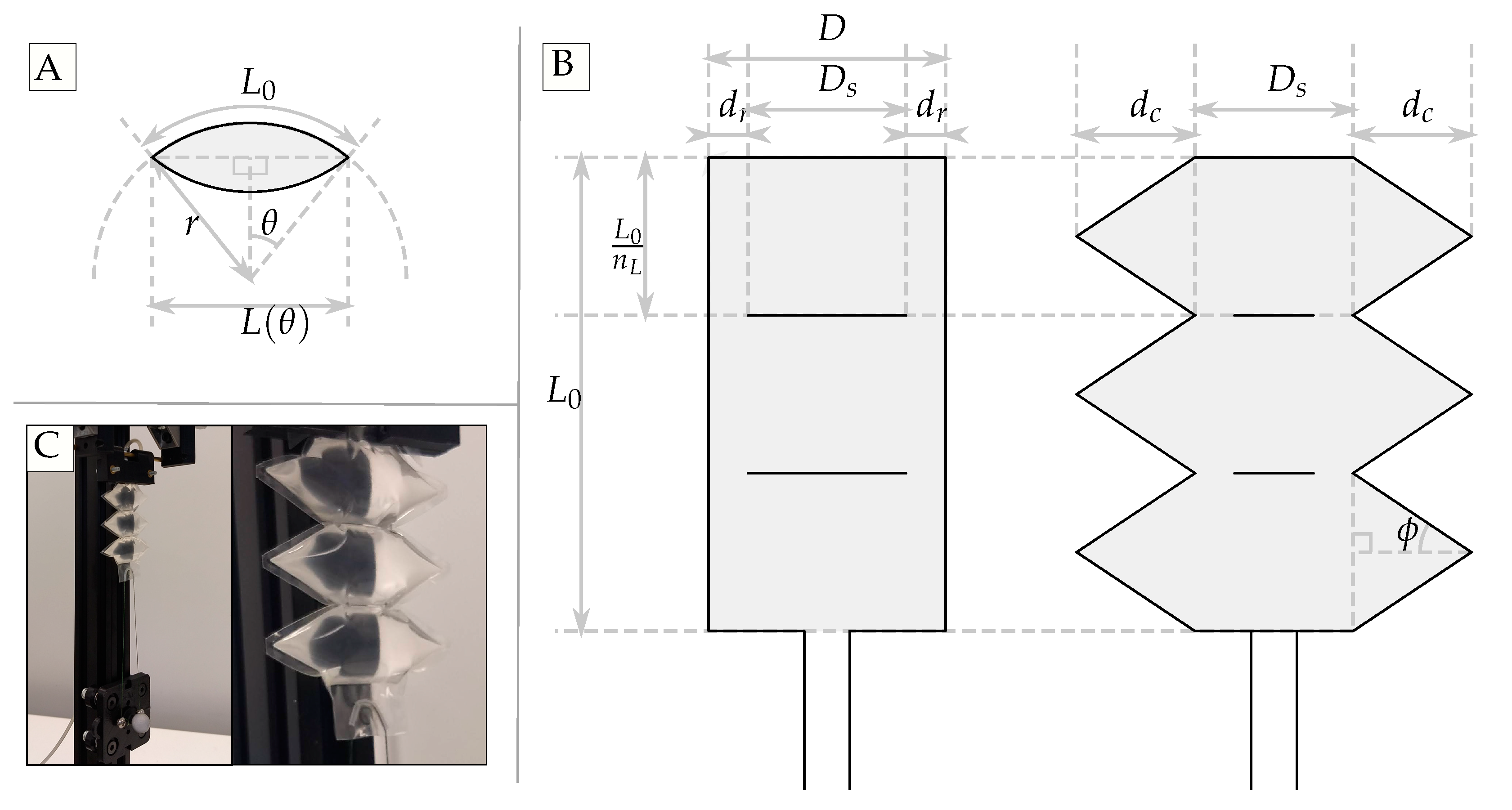
3. Materials and Methods

With reference to Figure 1, the parameters used to manufacture the actuators are shown in

Table 1. Actuator design parameters.

Parameter Name	Value
$n_L$	3
$L_0$	70.80 mm
$D_s$	20 mm
$d_c$	15 mm

. The value of $L_0$ was calculated before the operating range was defined, and an ideal actuator of this length would have been capable of 25 mm contraction. A total of 2 mm had also been added to the length to compensate for the width of the laser welded seams.

An important step towards achieving predictable contraction was to adjust for the difference between the theoretical volume and the real-world volume in the manufactured actuators. Note that this calibration step is distinct from the calibration step completed at the start of every test in order to zero the volume. The calibration to zero the volume is described with the pump hardware in Section 3.2.

The actuator was filled at a constant volume flow rate up to a gauge pressure of 75 kPa, while the contraction was monitored using an optical tracking system (Optitrack). The contraction was then plotted against the volume inside the actuator as shown in Figure 2.

The theoretical curve plotted in Figure 2 represents the ideal volume/length curve for an actuator with the geometry described in Table 1. The calibrated curve is defined by multiplying the theoretical volume by a factor, $k_v$, which in this case was equal to 0.815. The calibrated expression for volume of the actuator as a function of membrane curvature is therefore

$$\begin{array}{cc}\hfill V_c\left(\theta \right)& =k_v\frac{L_0^2}{n_L}\left(\frac{d_c}{3}+\frac{D_s}{2}\right)\left(\frac{\theta -cos\theta sin\theta }{{\theta }^2}\right)\hfill \end{array}$$

(3)

Note also that the actuator stopped contracting after it had been filled to a certain level. The contraction at which this happens for this specific actuator is approximately 18 mm, and this would inform the operating range of the actuators.

Two different considerations affected the minimum and maximum contractions and meant that constraints were placed on each in the control system. Firstly, it was observed that the maximum contraction, $L_{Cmax}$, could not be reached, and this may be because the membrane material had non-zero bending stiffness, non-zero thickness, and finite Young’s modulus. Secondly, when the actuator is contracted by only a small amount, the volume flow rate has to be high to achieve even low contraction speeds. Therefore, the minimum contraction was not set to zero to allow for reasonable actuation speeds when the actuators were used in antagonistic or parallel arrangements and the speeds must ‘match’.

In antagonistic and parallel arrangements, it may be the case that one actuator is contracted a little and can only move slowly, while another is significantly contracted and is able to move quickly due to the high volume change to length change sensitivity in this state. The actuation speed is therefore limited by the slower actuator as they must move together.

Consider that when a theoretical actuator is half full it will have contracted by only approximately 10% of its full potential stroke; conversely, when a theoretical actuator has contracted by half of its stroke, it will have to be filled to approximately 90% of its maximum volume.

3.1. Volume Estimation for Length Control

With reference to Equation (1), the function $sin\left(\theta \right)/\theta$, also known as the $sinc$ function in the field of signal processing, is bijective within the range $0\le \theta \le \pi /2$. Hence, for a given desired actuator length, $L\left(\theta \right)$, a single corresponding $\theta$ value can be found. Unfortunately, Equation (1) cannot be arranged to solve for $\theta$ directly because the function $sinc\left(\theta \right)$ has no simple inverse. Instead, lookup tables and linear interpolation were used to estimate $\theta$. Using the resulting value of $\theta$, the volume of the chamber required to reach $L\left(\theta \right)$ can be found using Equation (3).

3.2. Hydraulic Pumps and Control System

Syringe pumps are used to control the volume of water within each actuator. These can be modelled as fixed, positive displacement hydrostatic pumps. In each pump a stepper motor (NEMA 23 2305HS280AW, Ooznest) coupled to a lead screw drives a gantry along a linear stage. 3D printed adapters are used to hold both the syringe piston to the gantry and the body of the syringe (50 mL, BD Plastipak) to the linear stage. The end of the syringe piston was modified to reduce deformation under pressure, which would impact the volume inside the syringe body. The outlet of the syringe is connected via PVC tubing to a double tee joint where a pressure sensor (MS5803-14BA, TE Connectivity) is attached. A microcontroller (Arduino Uno, arduino.cc) controls the stepper motor using a stepper driver (DRV8825, Texas Instruments), reads the pressure sensor, and communicates with the control PC. Figure 3 shows the key components of the syringe pumps and part of the prismatic joint setup mentioned later.

The volume delivered to the actuator, expressed as $V\left(\theta \right)$ in Equation (3), is the current volume of the syringe minus the initial volume. A calibration procedure is therefore required, after which the initial volume in the actuator is assumed to be zero. The calibration step consists of retracting the syringe piston until a vacuum pressure is measured by the pressure sensor, in this case 85 kPa absolute. This negative pressure is maintained for 4 s to ensure that the actuator has indeed been emptied. The syringe piston must be stationary during this time because a transient vacuum gauge pressure could also be generated by resistance to flow.

The resolution of the syringe pump, $V_{res}$, is found by multiplying the cross sectional area of the syringe body with the resolution of the linear stage as in Equation (4). The resolution of the linear stage is determined by the lead, $L_{screw}$, of the lead screw; the number of steps per revolution, $S_{pr}$, of the stepper motor; and the number of microsteps, ${\mu }_{steps}$, used by the stepper driver. The syringes used had an inner radius, $r_{syringe}$, of 13.25 mm from which their cross sectional area could be calculated.

$$V_{res}=\frac{L_{screw}}{S_{pr}·{\mu }_{steps}}·\pi ·r_{syringe}^2$$

(4)

With $L_{screw}$ equal to 4, $S_{pr}$ equal to 200, ${\mu }_{steps}$ equal to 4, and $r_{syringe}$ equal to 13.5 mm, the resulting volume resolution is 5.516 mm${}^3$. The theoretical maximum volume is found by substituting $\theta =\pi /2$ into Equation (3) along with the appropriate parameters representing the actuator geometry, resulting in a maximum volume of 15,066.332 mm${}^3$. Therefore, 2731 steps would be required to fill the actuator to the theoretical maximum, rounded down to an integer number of steps.

3.3. Positioning Test Setup

Figure 4 shows diagrams of all the test setups tested.

3.3.1. Experimental Setup: One DOF

A single actuator was clamped at its proximal end where the inlet tube entered it and was suspended from a rigid support aligned with the centre of a v-slot aluminium linear rail. An optical motion tracking system (OptiTrack, NaturalPoint) was used to track a pair of retro-reflective markers respectively placed on the rail and on the moving linear stage. The first marker was a stationary reference marker aligned with the centre of the linear rail. The second marker was placed at the centre of a linear stage gantry plate that had low friction wheels and was constrained to move along the linear rail, with the distance from the marker to the rail equal to that of the first marker. The placement was to ensure that the relative motion of the markers was along a straight line connecting the two. Figure 4A shows this setup.

A block and tackle pulley delivers a mechanical advantage of 2, so the stroke of the actuator was doubled at the expense of half the force exertion. This was chosen because the hydraulic actuators were capable of exerting high forces and because their stroke is not large in proportion to their length.

To implement a block and tackle pulley, one end of the cable was anchored to the structure, in this case the aluminium rail, while the other end remained attached to the end effector, the linear stage. The PTFE tubing conforming to the circular weld in the actuator therefore became a capstan, as a substitute for a rotating pulley, with the cable wrapped around it by 180°. Due to the use of PTFE, the friction around the capstan was assumed to be zero. Figure 4B shows the pulley setup.

In the antagonistic setup, two identical actuators were clamped to the linear rail at either side of the linear stage and coupled to the linear stage. Retro-reflective markers were again placed at fixed locations relative to the actuators, with one marker at the centre of the linear stage. The linear stage was free to move a distance equal to the actuators’ stroke, and the actuators were spaced such that when one actuator was at its maximum contraction, the other would be at its minimum contraction. A diagram of the antagonistic setup is shown in Figure 4C.

3.3.2. Experimental Procedures: One DOF

The desired contraction of the actuator was alternated between the minimum and maximum contraction values of 2 mm and 17 mm using the hydraulic control system, pausing at each extreme thirty times. To test the actuators in a somewhat more realistic use case, a random positioning test was set up. The desired contraction was set to random values between the minimum and maximum contraction, to two decimal places, and with short pauses between moves.

3.3.3. Planar Parallel Mechanism

The entry points of the cables to the parallel mechanism’s workspace were arranged in an equilateral triangle as shown in Figure 4D,E. The cables are attached to a shaft intersecting the entry point plane, which is defined as the Y-Z plane. The cable entry points are at the end of capstans depicted in Figure 4 as point 8. Assuming that the connection to the shaft assembly stays in the plane of the entry points, the contact angle is equal to $\pi /2$. The friction from these capstans is assumed to be zero, as PTFE tubes were inserted for their entire length. Given this structure, the planar parallel mechanism is an RPR type [28], where the prismatic joints are actuated. The two passive rotary joints are found at the cable entry points to the structure and at the coupling to the shaft because in both places the cables were free to rotate.

The shaft coupling was designed such that the cables could rotate radially around the shaft while remaining perpendicular to it, depicted in Figure 4 as point 11. Each cable is attached to one of three nested pairs of rings that rotates independent of the others. This design meant that the point of intersection of the direction vectors of the cables was assumed to be in the centre of the shaft. Therefore, the cables were thought of as intersecting at a single point in the centre of the shaft, or, alternatively, the shaft could be thought of as having zero radius. In reality, each ring-pair of the cable coupling extends radially from the shaft and restricts the range of the actuators to a small degree. The coupling is also free to move axially along the shaft, meaning that the point of intersection of the direction vectors of the cables was assumed to exist in the entry point plane. The planar position of the point of intersection of the entry point plane, the shaft, and the three cables is controlled by the control system.

Retro-reflective markers were placed at both ends of the short shaft to which the cables were attached. As the position of both ends of the shaft could be tracked, the direction vector of the axis of the shaft could be determined. The point of intersection of the direction vector of the shaft with the entry point plane was recorded as the measured position.

A second support structure was constructed with an entry point equilateral triangle whose side length was double that of the first support structure. This was done because pulleys were again used to double the stroke of the actuators. The only difference between the two support structures other than the increased side length was the accommodation of a cable anchor point to create the block and tackle pulley.

3.3.4. Experimental Procedures: Two DOF

To test the capability to follow a predefined path, four different paths were constructed as series of equally spaced waypoints in the two-dimensional workspace. Three of the paths consisted of circles centred at the origin with diameters of 2.5 mm, 5 mm, and 7.5 mm, respectively. The last path was a raster scan pattern focused on the central portion of the workspace. The base of the raster scan pattern is equal to half the width of the equilateral triangle formed by the entry points and was centred with it.

3.4. Three DOF Positioning Tests

3.4.1. Experimental Setup: Three DOF

The two-DOF positioning method was used with a small number of modifications to add a third DOF, as shown in Figure 4G. These modifications were: a spherical coupling to attach the cables to the shaft; a telescopic shaft; and a rotary joint, or equivalent, that constrains the proximal end of the shaft. Three DOFs of the end effector are controllable: yaw, $\psi$; pitch, $\varphi$; and extension in the x direction.

As a result of the spherical coupling’s design, the direction vectors of the three cables are assumed to have a single point of intersection in the plane of the cable entry points of the structure. Therefore, controlling the position of the point of intersection can be achieved in the same way as in the two DOF tests.

A prismatic joint was added by incorporating an inner telescopic shaft to the existing shaft. To produce linear motion of the distal tip of the telescopic shaft along its axis, a motorised linear stage moves the instrument axially in relation to a Bowden tube.

By constraining the end of the shaft assembly with a rotary joint, the two prismatic DOFs of the shaft became rotational DOFs. A continuum joint was used, as both the size was small and friction with the telescoping instrument was low. The curvature was assumed to be constant along the length of the continuum joint. Furthermore, the length of the continuum joint was assumed to be constant.

3.4.2. Experimental Procedures: Three DOF

To validate the ability of the mechanism to position the tip of the shaft in three-dimensional space, various paths were set for the robot to follow. The paths filled a large portion of the workspace and included two circular patterns, a helix aligned with the X axis, an Archimedean spiral projected on a cone, and another Archimedean spiral projected onto a cylindrical surface. The simpler circular and helical paths were repeated 30 times, while the spiral patterns were repeated 10 times.

3.5. Force Exertion Setup

The force exertion of a single actuator was tested by blocking it at various levels of strain with the proximal end clamped to a support structure and the distal end coupled to a force sensor (ATI, Nano 17). The actuator was blocked at strains between 2 mm and 16 mm inclusive, at increments of 1 mm, and three repetitions of the test procedure were performed at each strain value. The maximum force in each of the three repetitions was recorded and the mean value recorded as the result. The pressure in the actuator was set at 120 kPa and 130 kPa absolute in two rounds of testing, respectively, with the volume being recorded during tests. Higher pressures could have been used, as other designs manufactured with the same method had burst pressures of over 250 kPa absolute.

4. Results

4.1. Positioning

4.1.1. One Degree of Freedom

Figure 5 shows the results of the one-DOF positioning tests. Diagrams of the one-DOF tests are shown in Figure 4A–C. The actuators follow the trajectories as expected, with the antagonistic setup appearing to be more accurate. Some lag was observed as the actuators took time to reach the desired targets and this seemed to be longer for the antagonistic actuators.

The root mean square error (RMSE) and hysteresis were calculated as appropriate for each test. For the minimum to maximum tests, the values were calculated across all points, whereas for the random positioning tests, only the times when the actuators were static were considered.

The hysteresis was calculated by taking the measured contraction on the forwards and backwards paths, then finding the maximum absolute difference of these values throughout the test. Figure 6 shows the hysteresis of the single actuator, antagonistic actuators, and the single actuator with a pulley. The RMSE, hysteresis values, and minimum and maximum percentage errors are summarised in

Table 2. Summary results table for each of the one-DOF tests.

Configuration	Test	RMSE/mm	Hysteresis	% Error
			/mm	+ve	−ve
Single	Min. to Max.	0.4713	0.7113	+6.25%	−4.12%
Single with pulleys	Min. to Max.	1.5062	0.9580	+7.48%	−1.34%
Antagonistic	Min. to Max.	0.3496	0.5145	+3.67%	−4.08%
Single	Random	0.3711	-	+4.23%	−4.75%
Antagonistic	Random	0.2632	-	+2.80%	−3.10%

.

4.1.2. Planar Parallel Mechanism

Figure 7 shows the path following results for the planar parallel mechanism setups. Some offset appears to be present, and this is most likely due to inaccuracy in the positioning of the actuator anchor points with respect to the entry point capstans.

Table 3. Summary table for results of each of the two-DOF tests.

		RMSE/mm		Max. Error Y/mm		Max. Error Z/mm
Configuration	Path	Y	Z	+ve	−ve	+ve	−ve
No pulley	Circle 2.5 mm ⌀	0.2818	0.4788	0.6360	−0.3016	0.2670	−0.8580
	Circle 5 mm ⌀	0.6705	0.5458	1.4873	−0.8085	0.9783	−1.1430
	Circle 7.5 mm ⌀	1.8396	1.5948	3.9157	−4.3145	3.6205	−3.9453
	Raster scan	3.3391	1.7345	10.0754	−8.8439	4.3930	−5.8534
Pulley	Circle 5 mm ⌀	0.3956	0.8915	1.0458	−1.0229	1.6253	−0.0897
	Circle 10 mm ⌀	0.5805	1.2137	0.7261	−1.5084	2.3462	−0.2917
	Circle 15 mm ⌀	0.5131	0.5003	1.4162	−1.2809	1.2756	−0.2438
	Circle 20 mm ⌀	0.8735	0.9833	2.6011	−2.2634	3.1025	−1.6103
	Raster scan	4.9296	0.9606	6.0424	−6.1034	3.5801	−3.5761

summarises the RMSE in the Y and Z dimensions, as well as the maximum errors.

The results with a pulley are comparable to or better than the results without a pulley, which is noteworthy given that the ranges of Y and Z were doubled. The maximum errors in the raster scanning patterns were large, although this was due in part to the end effector momentarily going out of synchronisation with the desired position.

4.1.3. Three DOF Hybrid Parallel Mechanism

Figure 8 shows the path following results for the rigid three-DOF system. The performance was again satisfactory despite the presence of some offset and triangular skew as described in the previous section. Due to the integration of the prismatic joint, some hysteresis was present in the X direction because of the friction experienced between the Bowden tube and the flexible rod. It is worth noting that avoiding the effects of friction was one of the motivations for developing the soft actuators.

The observed position in the helix path shows a deviation from the desired path when the path started again from the beginning, denoted by the straight line in the desired path aligned with the X axis. This occurred because there was no pause between the end and beginning of the repetitions, and as such, the prismatic joint position lagged the desired value significantly.

Table 4. Summary table for results of each of the three-DOF tests.

	RMSE/mm			Error X/mm		Error Y/mm		Error Z/mm
Path	X	Y	Z	max.	min.	max.	min.	max.	min.
Circle 10 mm ⌀ YZ	1.4866	1.7571	1.5900	1.7720	1.2182	3.6386	0.1624	3.6629	−0.4152
Circle 10 mm ⌀ at 45° pitch	0.7274	1.3102	1.4734	1.6933	−0.8127	2.8806	0.1970	3.2618	−0.2895
Helix 20 mm ⌀	5.0991	1.7962	1.8811	3.8503	−27.7232	5.0012	−2.4748	4.7601	−2.3074
Conic spiral 30 mm ⌀ base	2.3663	1.6742	2.1441	5.8209	−1.0461	2.6694	−4.5342	4.0849	−4.5019
Spiral on 20 mm ⌀ cylinder	2.5468	2.5980	1.5421	4.2084	1.4722	3.1964	−6.8052	4.5496	−2.9175

contains the RMSE in X, Y, and Z for the five different tests that were carried out, as well as the minimum and maximum errors. Note that the large RMSE and minimum error in X for the helix test was due to the transition from the maximum extension to the minimum, as shown in Figure 8C.

4.2. Force Exertion

Figure 9 shows the results of the force exertion tests. The force exertion was high across most of the operating range, and especially so at low contractions, as expected when considering the shape of the actuator and direction of the tension force. To exert a tension of T, the tension in each membrane of the chamber depends on $1/cos\left(\theta \right)$, which tends towards infinity as $\theta$ tends towards $\pi /2$. Higher pressures are required at higher strains to sustain the required membrane tension, thus the force exertion at high strains is low as the pressure is held constant.

4.3. Deployable Robot

A parallel robot was manufactured with an inflatable support structure as well as the soft actuators described above. Aside from the support structure, the components are all the same as the previous three-DOF setup—the continuum rotary joint, prismatic joint (telescopic shaft), and rotary shaft coupling. As such, the robot also controls the position of the tip in three spatial dimensions.

Figure 10 shows various angles of the deployable robot and the result of a human-in-loop path following task to trace a circle 30 mm in diameter. The support structure was pressurised with air at 200 kPa absolute during testing.

5. Discussion

Many technical challenges have to be faced in the field of MIS and new approaches are necessary to meet them. Soft robotics is a growing field of study that shows good potential to deliver benefits in comparison to conventional rigid robots in areas such as MIS where interaction with humans and human tissues is the focus. The aim of achieving open loop position control with a soft actuator was achieved. Furthermore, the actuators proved to be highly repeatable: in each of the positioning tests, the paths were traced either 30 or 10 times, and, as can be seen in the figures, almost exactly the same path was taken each repetition. Therefore, the actuators show potential for use in a surgical context, and, in addition, they are soft and compliant. To further show the viability of using the actuators in a surgical robot, a deployable robot was manufactured and tested. The robot showed excellent responsiveness, and tracing the 25 mm diameter circle in the test was an easy task, even without a camera system focused on the target to aid the user, or any other guidance. Pulleys were used to increase the stroke of the actuators and reduce their size, which has benefits in MIS where space is limited. The large workspace of the robot is adequate for ESD, where tracing paths around cancer lesions more than 20 mm across is an important step. Success in this test serves as an important proof-of-concept for robotic systems that use inflatable, deployable structures and actuators. Further research is needed to increase the accuracy of the actuators to a level adequate for MIS.

Both the structures and actuators were manufactured by laser welding thermoplastic sheets together in specific patterns. The result of this is that, when not inflated or filled with actuation fluid, the constituent parts are very flexible and low-profile. In addition, these parts are very economical to produce and could be made into single-use, customised robots.

The design of the robot could be improved, as bending in the structure was observed when the parallel mechanism neared the boundary. In fact, prototyping of deployable robots of different types would be valuable: for example, serial or hyper-redundant robots manufactured with the same method.

Regarding the actuators, the positioning results could also be improved by improving the calibration method or increasing the volume resolution of the pump, especially at higher contractions when sensitivity to volume change is high. The operating range could also be widened, as the limits were chosen heuristically in this work.

The hysteresis results were all under 1 mm even after adding a pulley and were lowest for the antagonistic setup. The antagonistic actuators were tested in a horizontal configuration, so there was no restoring force in the opposite direction to the contraction of either actuator. This may explain why there is a flat hysteresis profile throughout the stroke in comparison to the vertical configuration where the hysteresis varies with the stroke. Given that the positioning was highly consistent, it is expected that the hysteresis could be compensated for successfully.

A difference in the method to position the actuator anchor points may explain the difference in offset between the systems with and without pulleys. The approach used for the pulley mechanism appears to be superior. The slightly triangular paths traced may have been caused by friction in the rotary shaft coupling, or high tension in actuators as is common in parallel mechanisms as they approach their singular configurations at the boundaries.

In ongoing work, the minimum and maximum actuator speeds recorded were approximately 4 mm/s and 26 mm/s at the limits of the 2 mm–17 mm contraction operating range, respectively. The speed was measured in response to a step input in desired contraction from 0 mm to 17 mm.

The force exertion results compare well with [19,20,25], and their actuators were of a larger size, which increases force exertion. A single sub chamber in our design had dimensions $L_0$ and D of 22.67 mm and 30 mm, whereas these were 25 mm and 85 mm in [19], 40 mm and 160 mm in [25], and 20 mm and 40 mm in [26].

Due to the surface tension of the hydraulic actuation fluid and the associated pressure rise due to Laplace’s law, the measured forces exerted by the actuator do not follow the same relationship as the pneumatic actuators, and the Laplace pressure must be compensated for.

A liquid with low boiling point was used to fill an actuator in [29] that was later sealed such that, when heated, the liquid evaporates and contracts the pouch with no need for inlet tubes. The slow actuation speed and controllability make this less effective but would be interesting for untethered or wireless actuation. In [30], wireless actuation was achieved by heating the low boiling point liquid with a laser, which evaporates the liquid and induces contraction.

Future work will include finding an expression for the force exertion in terms of the membrane curvature $\theta$ and the internal pressure. This could be used to sense the forces exerted on the actuators based on the hydrostatic pressure. The hydraulic supply tubes used were 0.5 m in length, but for endoscopic applications, the supply tubes would measure approximately 2 m, which would increase the resistance to flow in dynamic situations. Poiseulle’s law could be used to compensate for transient pressure changes due to flow, but this would represent a more complex problem. However, in static situations the pressure could be used to estimate forces as in [31], for example.

Sensorising the actuators using approaches from electrical impedance tomography (EIT) as in [32] to achieve closed-loop position control is another area of investigation. Adding this type of sensor would also facilitate detection of external disturbances. A simpler technique is to use a conductive working fluid and monitor changes in the resistance as in [33], which is also a viable option for these hydraulic actuators. However, one of the advantages of this type of actuator is the low-profile, low-cost construction; therefore, a simple open loop control strategy was implemented that required neither bulky sensors nor intensive computation or modelling.