Automatic Classification of A-Lines in Intravascular OCT Images Using Deep Learning and Estimation of Attenuation Coefficients

Abstract

Intravascular Optical Coherence Tomography (IVOCT) images provide important insight into every aspect of atherosclerosis. Specifically, the extent of plaque and its type, which are indicative of the patient’s condition, are better assessed by OCT images in comparison to other in vivo modalities. A large amount of imaging data per patient require automatic methods for rapid results. An effective step towards automatic plaque detection and plaque characterization is axial lines (A-lines) based classification into normal and various plaque types. In this work, a novel automatic method for A-line classification is proposed. The method employed convolutional neural networks (CNNs) for classification in its core and comprised the following pre-processing steps: arterial wall segmentation and an OCT-specific (depth-resolved) transformation and a post-processing step based on the majority of classifications. The important step was the OCT-specific transformation, which was based on the estimation of the attenuation coefficient in every pixel of the OCT image. The dataset used for training and testing consisted of 183 images from 33 patients. In these images, four different plaque types were delineated. The method was evaluated by cross-validation. The mean values of accuracy, sensitivity and specificity were 74.73%, 87.78%, and 61.45%, respectively, when classifying into plaque and normal A-lines. When plaque A-lines were classified into fibrolipidic and fibrocalcific, the overall accuracy was 83.47% for A-lines of OCT-specific transformed images and 74.94% for A-lines of original images. This large improvement in accuracy indicates the advantage of using attenuation coefficients when characterizing plaque types. The proposed automatic deep-learning pipeline constitutes a positive contribution to the accurate classification of A-lines in intravascular OCT images.

1. Introduction

Atherosclerosis is the main cause of morbidity and mortality in developed countries. It is a complex, progressive disease of the arterial wall, resulting in life-threatening thrombotic episodes such as acute coronary syndromes. More than 75% of plaques that result in acute myocardial infarction and/or death are non-stenotic [1]. Numerous studies based on histology and intravascular imaging techniques have tried to detect the type of atherosclerotic plaque that results in an acute coronary syndrome, whose most frequent mechanism is plaque rupture [1,2]. This prone-to-rupture type of plaque is characterized as “high risk” and has specific morphologic features: a thin fibrous cap that covers a large superficial lipid pool and often exhibits local signs of inflammation [2,3,4].

Optical coherence tomography (OCT, intravascular OCT) is a light-based medical imaging modality. It was first demonstrated by Huang D et al. in 1991 [5]. In intravascular imaging, OCT has been established as the frequency or Fourier domain (FD—OCT) system due to the advantages it presents (in terms of speed and sensitivity) [6,7]. In recent years, continuous improvements in the technology of OCT systems, mainly in terms of the Micro-Electro-Mechanical Systems (MEMS) [8], have allowed their easy application in the study of biological tissues and the achievement of an axial resolution <2 μm.

In Intravascular Optical coherence tomography, the light is in the near infrared (NIR) range, typically with wavelengths of approximately 1.3 μm, which provides a 10-fold higher spatial resolution than that of intravascular ultrasound (IVUS), allowing the precise measurement of the fibrous cap thickness and detection of plaque components. OCT can be used to identify various stages of plaque morphology. The main limitation of intravascular OCT is the limited penetration depth in the artery wall, as it depends on tissue type and usually ranges from 0.1 to 2.0 mm using typical IVOCT NIR light.

Intravascular OCT can identify several types of atherosclerotic plaques. According to the published expert consensus documents, an atherosclerotic plaque (atheroma) in intravascular OCT images is defined as a mass lesion (focal thickening) or loss of a layered structure of the vessel wall. A fibrous plaque has high backscattering and a relatively homogeneous intravascular OCT signal. A calcific plaque contains intravascular OCT evidence of calcium that appears as a signal-poor or heterogeneous region with a sharply delineated border (leading, trailing, and/or lateral edges). This definition applies to larger calcifications. A lipid plaque by intravascular OCT is a signal-poor region with poorly delineated borders, a fast signal drop-off and little or no signal backscattering, covered by a fibrous cap. Mixed lesions are called heterogeneous plaques or mixed lesions [9,10].

The assessment of the degree of the development and the type of plaque is very important for identifying high-risk plaques. The use of OCT involves the collection of a large amount of imaging data (e.g., 100–300 cross-sectional images are collected for each artery), the examination of which requires a lot of time and great effort from a skilled medical specialist. Besides, it can be very hard to distinguish plaques even for experts on the field [9,11]. Therefore, an automated method is needed to detect and categorize the microstructures of interest and objectify the characterization. Athanasiou et al. [12] demonstrated that automatic characterization methods can provide accurate results despite the propagation of error caused by the image formation, the intermediate steps, and the final classification phase of such methods.

The aim of this work is the development of a new deep learning method to detect atherosclerotic tissues in intravascular OCT images. Steps for the classification of detected plaques into four categories are proposed. The method is based on the classification of the A-lines into normal and abnormal (tissues) and the differentiation of the abnormal tissues into four plaque types. The main idea is to configure the input to a CNN architecture and to choose CNN properties and training options that offer better classification results.

The present paper is structured as follows: In Section 2, we discuss related work. In Section 3, we refer to the material of the study and describe the proposed method in detail. Section 4 presents the obtained results. In Section 5, we discuss the methodological approach and the outcomes of the study. Finally, Section 6 presents the conclusions of the study.

2. Related Work

Several methods attempted to automatically detect specific plaque regions. Wang et al. [13] proposed an automatic method for lumen segmentation and calcified plaque detection. The first task is achieved by a dynamic programming scheme and the latter by combining edge detection with active contour models. Other approaches apply machine learning techniques based on hand-crafted or automatically extracted features. Specifically, Shalev et al. [14] used hand-crafted features to train Support Vector Machines (SVM) and Radial Basis Function (RBF) classifiers to discriminate calcifications, lipid plaques, and fibrous tissue/plaque (one grouped category). Similarly, Athanasiou et al. [15] used hand-crafted features to train SVM, neural networks and Random Forests (RF) classifiers to classify the detected plaque into four types: calcified, lipid, mixed, and fibrous tissue. Random Forests provided the best classification results. It is not clear, however, if the last type refers to fibrous plaque or normal fibrous tissue. Prakash et al. [16] proposed an unsupervised classification approach that uses the K-means clustering algorithm applied to statistical texture features to identify background, plaque, and normal tissue areas. Their method provided a rough estimation and was evaluated by visual inspection.

Instead of using hand-crafted features, other studies applied deep learning to OCT cross-sections or patches, attempting a semantic interpretation. Gessert et al. [17] used ResNet and DenseNet to classify OCT images in three categories: normal with calcified plaque and with fibrous or lipid plaque. This method does not classify image regions but whole images. Oliveira et al. [18] applied a fully connected CNN known as SegNet. The dataset consisted of 51 images of 13 patients. Patches of 100 × 100 pixels were input to SegNet, which produced a probability map with two classes: normal and calcified plaque. Probabilities derived from overlapping patches were combined in post-processing steps to classify each pixel of the image. The accuracy was 0.7 in this task. He et al. [19] presented a method that applied an original CNN to 269 images of 22 patients. Images were divided into square patches of 51 × 51 pixels, which were used to train the network. They chose to classify tissue in 4 categories (neglecting fibrous plaque). The accuracy of the algorithm in detecting calcified plaque was too low, resulting in Dice = 0.22. Most of the existing methods are patch-based (pixel classification), having several limitations. Plaque types are not considered, e.g., fibrous plaque. Moreover, it is uncertain if these methods can generalize to other images because there is no reference to data handling and splitting into training, validation, and test sets. Generally, patch-based approaches have difficulty achieving tissue classification because some plaques present similar textures. In addition, the stratification of artery wall layers (intima, media, and adventitia), which is not depicted in patches, is more indicative of the presence of plaque structures.

Therefore, several methods were proposed for axial line (A-line) classification. A-line classification does not permit the delineation of plaque structures, which is attempted by patch-based methods. However, it permits the estimation of the extent of the plaque present on the arterial wall. Rico-Jimenez et al. [20] modeled every axial line in IVOCT data as a linear combination of several depth profiles. After the estimation of these profiles through least-square optimization, they classified the tissue types based on their morphological features. While they examine four A-line types—Intimal-thickening, Fibrotic, Superficial-Lipid, and Fibrotic-Lipid—their method was tested in ex vivo data and was successful in discriminating lipid and non-lipid tissue (85%). Prabhu et al. [21] applied dual binary classifiers and SVM to features extracted from A-lines to achieve 81.56% accuracy in three-way classification. Kolluru et al. [22] applied deep learning combined with Conditional Random Fields to achieve 83.16% accuracy in the same task. Lee et al. [23] built upon these methods and enhanced their performance (89% accuracy) by introducing lumen morphology features and active learning. Abdolminalfi et al. [24] used a CNN to extract features from A-lines. These features were input to three classifiers (neural networks, random forests, SVM) and trained to distinguish intima and media in the arterial wall. The outcome of this method is related to the detection of plaques because the clear appearance of intima and media layers is indicative of healthy tissue. Therefore, Zahnd et al. [25] proposed a method that, after detecting the layers of the arterial wall, determined if wall parts (series of A-lines) are healthy or diseased, and they had 0.91 median accuracy. Their dataset consisted of 260 images, but it was imbalanced (containing mostly healthy tissue).

One aspect of plaque detection and plaque calcification to be considered is the use of optical-transformed images instead of intensity images acquired by OCT systems. Boi et al. [26] published a review of deep learning IVOCT approaches, including methods for the calculation of backscattering and the attenuation coefficients of tissue in OCT images. It is suggested that these methods may enhance performance in plaque detection and plaque classification tasks. One of these methods was the study of van Soest et al. [27], who highlighted attenuation coefficient’s importance for tissue classification and modeled it with more accuracy. Foin et al. [28] showed that the estimation of the attenuation coefficient leads to better manual segmentation by medical experts. Liu et al. [29] expanded van Soest et al.’s work and presented a detailed method for the estimation of backscattering and attenuation coefficients. Liu et al.’s [29] formulas were used in the present work.

3. Materials and Methods

3.1. Materials

We studied 183 intravascular FD-OCT images derived from 33 patients who underwent a clinically indicated cardiac catheterization. All imaging data were blindly acquired at Hippokration Hospital, Athens, Greece, General Hospital of Nikaia, Piraeus, Greece and New Tokyo Hospital, Chiba, Japan, using standardized image acquisition protocols.

The OCT acquisition was performed with a frequency-domain OCT imaging system (C7-XRT OCT Intravascular Imaging System, Westford, MA, USA) at a pullback speed of 20 mm/s, axial resolution of 15 μm, and maximum frame rate of 100 frames/s. Temporary blood clearance was achieved with contrast infusion. Expert cardiologists annotated 183 images with tissue and plaque types according to the standards of published consent of experts [9]. Plaques that appeared in the annotated images were: 84 lipid, 80 calcified, 70 fibrous, και 42 mixed.

3.2. Methodology Overview

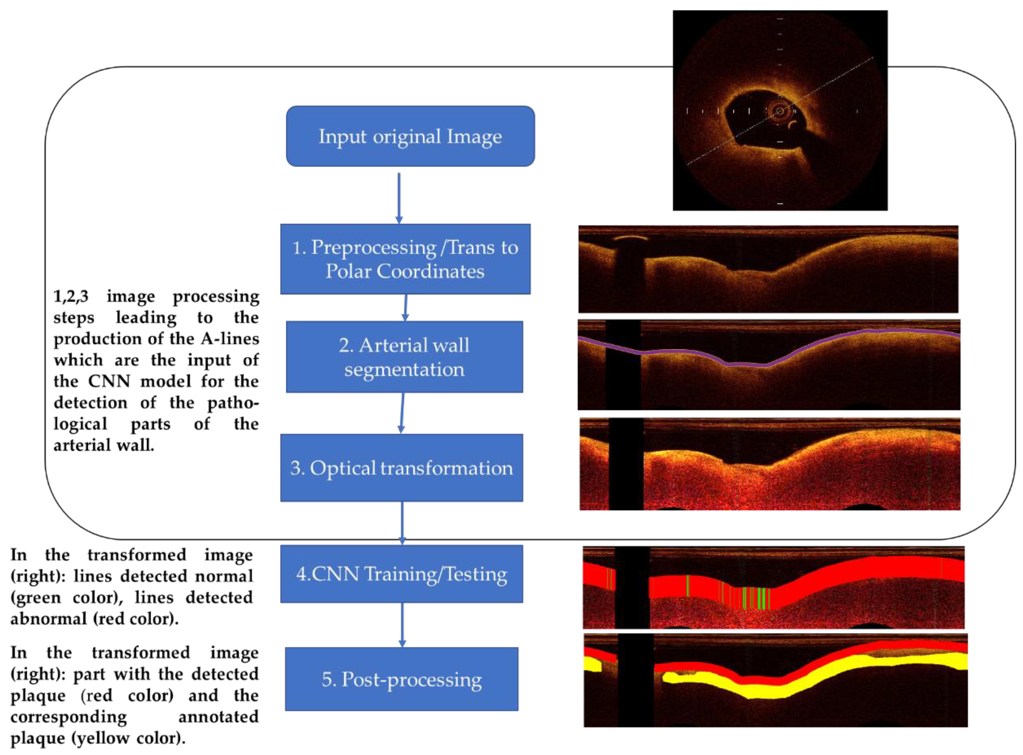
A-line is the propagation line of the light beam that starts from the catheter and reaches the depth of the biological tissue where it is completely attenuated. The method, which classifies A-lines to normal and plaque, consists of the following analysis steps: (1) preprocessing—image preparation, (2) arterial wall segmentation, (3) OCT-specific transformation based on the attenuation coefficient estimation, (outcome the A-lines that are input to the CNN), (4) CNN training—testing procedure (for the detection of the pathological tissue and classification of the different tissue types), and (5) post-processing based on the majority of the classifications. The employed image processing and CNN classification procedure workflow is illustrated in Figure 1 and described below.

3.3. Preprocessing

Preprocessing steps included: (i) dataset “alignment” by image resizing, (ii) calibration markers’ noise removal, and (iii) polar coordinates transformation:

Due to the fixed size of the CNN input and to the examination of texture features, images were “aligned”, i.e., they were resized to have the same size and resolution. Most images in the dataset used had the size of 1024 × 1024, and we chose to oversample smaller images. Few images in our dataset had higher resolution than 2048 × 2048 pixels. We chose to downsample the latter because oversampling all other images of the dataset to their size would significantly alter the original data.

Calibration markers represent non-natural pixels in the images and were thus removed. The intensities of pixels in calibration markers’ positions were estimated by taking the median value of their region utilizing a 5 × 5 window.

The transformation of images to polar coordinates was proposed by several studies [12,13] both for the delineation of arterial wall-lumen border and for semantic analysis by deep learning techniques. In this work, this transformation was also an essential step to achieve these tasks and to extract A-lines that are input to the proposed deep neural network architecture. Given a pixel (x,y) in the Cartesian domain, its corresponding position (ρ,θ) in polar coordinates is given by [30]:

x = Cx + ρ*cos(θ) and y = Cy +ρ*sin(θ)

(1)

where (Cx,Cy) is the image center coordinates (the central point of the catheter) in the Cartesian domain. We considered that we have enough information from the image in the Cartesian domain to represent a depth of 383 pixels and 1532 angles. Consequently, the size of the resulting images in polar coordinates was 383 × 1532 pixels.

3.4. Segmentation of the Arterial Wall

After preprocessing, the ARC-OCT algorithm was applied for the delineation of lumen-wall borders [30]. ARC-OCT includes mainly OCT-specific (depth-resolved) transformation of images, thresholding, morphological operations and contour smoothing. The lumen-wall border was not defined in A-lines with guide-wire artifacts, but it is estimated by the neighboring parts of the border. However, image parts influenced by guide-wire artifacts were excluded from further examination in this work. In Figure 2, the result of the lumen segmentation algorithm is presented.

The delineation of the lumen-wall border is equivalent to arterial wall segmentation with the assumption that what is deeper than the lumen-wall border and up to the point where there is no backscattered signal is considered the arterial wall. The arterial wall is the region where plaques and normal tissue can be found. Therefore, we applied ARC-OCT to produce one-dimensional A-line patches that start at the lumen-wall border and include pixels from the arterial wall. Each A-line patch acquired a tag, if at least one pixel is part of a manual delineated plaque. The tags were: fibrous plaque, lipid plaque, calcified plaque, mixed plaque, or normal tissue.

3.5. A-Line Size Selection

The penetration depth (how deeply within the tissue we can obtain OCT image data) usually does not exceed 2 mm in coronary arteries. At this depth, the light signal is usually completely attenuated. Medical experts suggested that 1.5 mm is the penetration depth on the arterial wall where information about tissue properties can be found in any case. This depth corresponds to 90 pixels in the dataset’s resolution [9]. We carried out relative tests with A-lines of different sizes (120, 110, 100, 90, 80, 70, and 60 pixels) to verify that A-lines of a 1 × 90 size are a reasonable option. Finally, we chose the A-line size of 90 pixels as input in our CNN model.

3.6. Attenuation Coefficient Estimation

Backscattered light, which forms the OCT image, is attenuated in arterial wall parts. Consequently, intensities of the same tissue type, e.g., endothelial, diverge. However, it is preferable that regions of a certain tissue type share a similar appearance. The latter is attempted by estimating attenuation coefficient values in every pixel of an OCT image. The outcome image is more realistic, i.e., a specific tissue type is represented by a smaller range of intensities while maintaining texture information. To test the effect of using the attenuation coefficient in the classification of A-lines, transformations of OCT-images were carried out according to the work presented by Liu et al. [29]. The attenuation μ in every pixel of an OCT image can be estimated with the OCT image intensities by using the formula [29]:

$$\mathsf{\mu }[\mathrm{i},\mathrm{j}]=\mathrm{I}[\mathrm{i},\mathrm{j}]/(2*\mathsf{\Delta }*{\mathsf{\Sigma }}_{\mathrm{n}=\mathrm{j}+1}^{\infty }\mathrm{I}[\mathrm{i},\mathrm{n}])$$

(2)

where I[i,j] is the intensity in the original image; Δ is the physical size of a pixel (mm/pixel); i indicates the A-line number; j indicates the depth. In the rest of this document, transformed images are often referred to as attenuation images for brevity.

In Figure 3, an example of these transformations is presented. In the Section 4, we show that A-line patches extracted from images representing estimated attenuation coefficient values are classified with higher accuracy than A-line patches extracted from images with original intensity values.

3.7. Deep Learning

CNNs are neural networks with convolutional layers followed by dense layers. CNN-based methods outperformed other methods in many computer vision problems. Specifically, accurate methods in A-line classification in IVOCT images [22,23] are using CNNs. Therefore, in this work, various original (trained from scratch) and pretrained CNN architectures were tested.

Pretrained CNNs are fixed, open-source methods that were trained with natural images. They can be efficient in medical image analysis by fine-tuning their parameters [31]. Fine-tuning the parameters leads to faster convergence during training than training from scratch. Such a pretrained network is AlexNet [32], which consists of five convolutional layers with rectified linear unit (ReLU) activations and three dense layers. Some of its activations are followed by max-pooling layers. Although there are more efficient architectures, AlexNet is still a basis for the development of simple architectures that are more easily trained due to their small number of layers.

Having been trained with natural images that are included in large databases, pretrained networks may not be suitable for medical images that represent the interior of the human body. Besides, resizing images to fit these networks may significantly alter their original representation. More specialized networks are needed for medical image analysis. In medical image analysis, regions are segmented based on their texture. When there is no abundance of images, semantic methods are not efficient. Therefore, images are segmented to fix-sized patches. This introduces the need for CNN architectures with smaller input sizes than state-of-the-art architectures. To analyze CT images of lungs, Anthimopoulos et al. [33] proposed an original CNN that is specialized in classifying small parts of the images. The main characteristics were: five convolutional and three dense layers. This network could be considered a miniature of AlexNet, but it does not use pooling layers.

Inspired by common architectures such as AlexNet and the more specialized miniature network by Anthimopoulos et al. [33] and after experiments with different CNNs, in this work, we propose the use of a 1-D CNN that takes as input axial-lines with the corresponding attributes (Figure 4. To test the nearly optimal depth of A-lines for classification, the input size varied from 1 × 60 × 3 and 1 × 120 × 3 by changing the size of the second dimension by 10 pixels each time. The resulting network we finally propose has input 1 × 90 × 3. It consisted of 3 convolutional layers, 2 dense layers, and an output layer. The size of the convolutional kernels was small to keep small the receptive field so that high spatial frequencies stimulate the kernels. Their exact size of 1 × 4, 1 × 2, 1 × 10 was chosen after experiments. In these experiments, the number of feature maps in each layer was also examined. The use of only one big dense layer accelerated convergence. A much smaller dense layer followed to capture A-line appearances that could be grouped in few categories. Overfitting was dealt with dropout layers after the dense layer and with L2 regularization (The L2 parameter was set equal to 0.0005). After experimentation with activations, leaky ReLU [34] was selected for the convolution layers. Leaky ReLU activation is more robust when applied to the convolutional layers. The last dense layer was followed by a softmax activation. The Adam optimizer was used to reduce categorical cross-entropy [35]. Hyper-parameter tuning was used to select the learning rate to be equal to 0.001. After 200 iterations without improvement of the training error, the training stopped.

With this architecture as a basis, deeper CNNs were examined, and their results were compared. These CNNs also converged fast and achieved a similar validation and test accuracy for each task. However, the architecture in Figure 4 (and

Table 1. Elements of the proposed CNN architecture.

	Name	Type	Activations	Learnables
1	Image input 90 × 1 × 3images with “zerocenter”normalization	Image input	90 × 1 × 3	-
2	Conv_1 32 4 × 1 × 3 convolutions with stride [1 1] and padding [0 0 0 0]	Convolution	87 × 1 × 32	Weights 4 × 1 × 3 × 32 Bias 1 × 1 × 32
3	leakyrelu_1 Leaky ReLU with scale 0.01	Leaky ReLU	87 × 1 × 32	-
4	Conv_2 32 2 × 1 × 32 convolutions with stride [1 1] and padding [0 0 0 0]	Convolution	86 × 1 × 32	Weights 2 × 1 × 32 × 32 Bias 1 × 1 × 32
5	leakyrelu_2 Leaky ReLU with scale 0.01	Leaky ReLU	86 × 1 × 32	-
6	Conv_3 32 10 × 1 × 32 convolutions with stride [1 1] and padding [0 0 0 0]	Convolution	77 × 1 × 32	Weights 10 × 1 × 32 × 32 Bias 1 × 1 × 32
7	leakyrelu_3 Leaky ReLU with scale 0.01	Leaky ReLU	77 × 1 × 32	-
8	fc_1 5 fully connected layers	Fully Connected	1 × 1 × 5	Weights 5 × 2464 Bias 5 × 1
9	fc_2 2 fully connected layers	Fully Connected	1 × 1 × 2	Weights 2 × 5 Bias 2 × 1
10	Softmax softmax	Softmax	1 × 1 × 2	-
11	Classoutput crossentrophyex with classes “1” and “2”	Classification Output	-	-

) slightly surpasses, in most cases, the performance of other deeper CNNs. In the Results section, we refer to its performance except for a comparison with a deeper CNN. In the latter case, two more convolutional layers were added as dropout layers following the convolutional layers.

3.8. Post-Processing

The similar performance of the CNN architectures in the normal/abnormal classification case is attributed to the descriptive properties of the data. Many A-lines were correctly classified as normal or abnormal with different CNN architectures. On the other hand, a smaller percentage of A-lines are misclassified. The test set includes information about the adjacency of A-lines. Based on the minimum extent of plaques, which is 40 A-lines, and the fact that a single normal A-line cannot reside inside a plaque region, it is assumed that an individual A-line, which is not classified as belonging to the same class with most of a group of 20 adjacent A-lines, is misclassified. Therefore, a post-processing step to smooth classification results and correct misclassifications was introduced.

Specifically, let the notation of classification be: C(i) = 0 (normal) or 1 (plaque), where i is the A-line number. For i = 1, 21, 42, …, M (where M is the total number of A-lines in an image): C(i:i + 20) values are updated to 0 if Σ(C(i:i + 20) ≤ 10 and C(i:i + 20) are update to 1 if Σ(C(i:i + 20) > 10. This step decides the classification result of an A-line based on the dominant class of the classification results of adjacent A-lines. This produces a more realistic outcome, and it can improve test accuracy by 1–2% in most cases. An example of a post-processing result is shown in Figure 5.

3.9. Experimental Setup

All experiments were performed on a laptop computer featuring an Intel Core i7-4720HQ 2.60 GHz CPU, 8 GB RAM memory and a 3GB NVIDIA GeForce RTX 1080 GPU. The algorithms were implemented in MatLab (2020a, MathWorks, Natick, MA, USA).

Regarding the evaluation of the method, five-fold cross-validation was used: from 183 cross-sectional images of coronary images of 33 patients, 6 groups were randomly selected. Each group consisted of images of 5 different patients, apart from one group that consisted of images of 3 patients. To assess the efficiency of the proposed pipeline, 5 rounds of tests were applied. In each run, one of the aforementioned groups was used as the validation set, one as the test set, and the remaining images were used as the training set. Training, validation, and test sets combined consisted of 196,580 A-lines (11,333 calcified, 39,956 fibrous, 17,724 mixed plaque, 40,183 lipid plaque, and 87,384 normal tissue).

4. Results

4.1. Classification to Plaque or Normal Tissue

In this section, we present results from experiments that classify A-lines as normal or abnormal with respect to three factors: A-line size, oct-specific transformation, post-processing. For each case, accuracy, sensitivity, and specificity were calculated based on the true positive, false positive, true negative, and false negative A-line classifications.

4.1.1. Impact of OCT-Specific Transformation

In

Table 2. The mean test accuracy (sensitivity/specificity) ± their standard deviation of A-lines (1 × 90) classification for original images and attenuation images.

A-Line Classification	Accuracy	Sensitivity	Specificity
Original Images	73.73% ± 5.65%	88.68% ± 1.41%	54.03% ± 10.25%
Attenuation Images	74.73% ± 6.55%	87.78% ± 8.79%	61.45% ± 8.4141%

, the mean accuracy, sensitivity, and specificity (from 5 cross-validation runs) are presented for original images and images corresponding to the attenuation coefficient. The results presented are the outcome of the full pipeline (including post-processing). It is observed that sensitivity is higher than specificity whether the input is the attenuation or original images. The specificity is higher in the classification of A-lines extracted from attenuation images than in the classification of A-lines extracted from original images. Therefore, less normal A-lines are classified as abnormal in attenuation images. Low specificity values can be attributed to artifacts and to non-detailed annotation. This is further analyzed in the Section 4.1.3.

In

Table 3. The best test accuracy of A-lines (1 × 90) for original images and attenuation images.

A-Line Classification	Simple Shallow Architecture	Deeper Architecture
Original Images	78.43%	78.92%
Attenuation Images	82.52%	78.59%

, the test accuracy is presented for different inputs (original images and attenuation images). From this table, it can be concluded that transformed images representing attenuation coefficients can improve classification results. The best test accuracy with original images was 78.79%, while the best validation accuracy with images representing attenuation coefficients was 80.83%. The settings and the CNN were identical in both cases (only the input was different). The contribution of transforming the images is more significant in four-way plaque and binary classification described in Section 4.2.

In the test runs that correspond to Table 2 and Table 3, the difference between training and test accuracy is not large as a mean value. For a specific test run, the mean training accuracy was 75.87%, while the mean test accuracy was 74.73%. A confidence interval of −4.4712% to 5.9712% of the difference was calculated. Therefore, overfitting is not significant, and effort must be focused on reducing both training and test error. However, it is important to stress that the results of the experiments carried out suggest that adding two convolutional layers and a dropout layer and altering hyperparameters does not significantly affect the classification results.

4.1.2. Impact of Post-Processing

The test accuracy mentioned until now is calculated after the post-processing step described in Section 3.7 is taken. However, all tests were also carried out without post-processing. There was a slight improvement in accuracy when using a post-processing step, e.g., for the run with best results, the accuracy was improved from 79.99% to 82.52%.

4.1.3. Visualization of Results and Annotation Issues

During annotation, only plaque regions were manually segmented. The rest of the regions of the arterial wall were considered normal. However, this may not always be the case. Medical experts annotate what they consider as most interesting plaque regions, e.g., a calcified plaque can be adjacent to fibrous plaque, which is extended to more A-lines than calcified plaque. In this case, A-lines corresponding to fibrous plaque may be wrongly classified as normal in our initial setup. This is in accordance with the results in Figure 6, where one can observe specific patterns of appearance in normal A-lines (true negative). These patterns are absent in A-lines that were classified as plaque but are not initially annotated as such (false positive). Therefore, a number of these A-lines may be part of non-annotated plaque or an artifact. To cope with these cases, an active learning process is proposed by Lee et al. [23]. In such a case, other medical experts blind to the initial expert annotation re-evaluate the automated method’s result. Still, even after applying the active learning process, there are many challenges to be addressed in the manual annotation of OCT images in both research and clinical practice [7].

Figure 7 shows plaque detection results for intravascular OCT test images containing three different plaque types. Visual inspection of the results showed that most A-lines that are falsely not classified as plaque are part of the fibrous plaque class. It should be noted that fibrous plaque having a similar texture with normal tissue is usually more difficult to discriminate from the latter. In general, however, there was a high degree of agreement between automatic and manual segmentation in locating the arteriosclerotic plaques.

Although plaque regions may be missed by manual segmentation, it is considered that those that are delineated are accurately labeled as fibrous, calcified, mixed, or lipid. Therefore, we examined the classification in the latter four plaque types, excluding the normal A-lines.

4.2. Plaque Classification

In this section, we present results from experiments that classify A-lines to plaque type. Normal A-lines are excluded. We examined the difference in results when input is original or attenuation images.

4.2.1. Four-Way Plaque Classification

Very few studies which attempt an automatic classification of tissue in OCT images discriminate four plaque types. To the best of our knowledge, there is no study for A-line classification that distinguishes four plaques. We performed five runs of four-way classification with different test sets of attenuation images. This procedure was repeated for original images. Cumulative confusion matrices were calculated for original images and attenuation images by adding the confusion matrices of five test runs. The accuracy was calculated from the cumulative confusion matrices. The overall accuracy was 53.47% for the attenuation images and 47.68% for the original images. In Figure 8, the cumulative confusion matrix of the five runs is presented for the attenuation images.

It can be observed that lipid and fibrous plaque are more often mistaken for each other. This is because A-lines often include both plaques. Fibrous plaque starts on the surface of the arterial wall and is followed by lipid plaque, which is located deeper. In fact, A-line classification methods refer to their combination as fibrolipidic plaques. Mixed and calcified plaques are also mistaken for each other because they present similar textures, and their tissue types share common properties. However, the borders of calcified plaque are sharply delineated. Border information is not captured by A-line classification. Therefore, A-line classification methods [22,23] probably refer to mixed and calcified plaques as one group, i.e., fibrocalcific plaque.

4.2.2. Classification to Fibrolipidic and Fibrocalcific

Similar to the previous classification, we performed ten runs of binary classification with different test sets each time. Five runs were carried out with A-lines from original images, and five runs were carried out with A-lines for attenuation images. Overall accuracy was calculated from the cumulative confusion matrices. The accuracy was 83.47% for A-lines derived from attenuation images and 74.94% for A-lines derived from original images. In the binary classification between fibrolipidic and fibrocalcific classes, the contribution of attenuation optical transformation is more significant than in classification into normal and plaque A-lines.

5. Discussion

Most methods presented in Section 2 do not consider all the plaque types that can be identified in OCT images by medical experts [9]. More often, these methods do not distinguish fibrous plaque. Our study includes two more types of plaque than the previously mentioned works [22,23]. Specifically, we considered four plaque types: fibrous, lipid, calcific, and mixed. A-line classification methods were based on a quite arbitrary outer wall border segmentation to select the input (A-line patch) to the classifier. Alternatively, other methods used whole A-lines (from the catheter to maximal depth). We selected A-line patches that start from the arterial lumen-wall border and include pixels that are part of the arterial wall. Instead of choosing an endpoint pixel at a certain depth, we compared the classification results of our pipeline giving as input A-line patches of different sizes. In addition, inspired by the work of Boi et al. [26] and using Liu et al. [29] approach, we estimated the attenuation coefficient in every pixel of each image. The outcome images offered better A-line classification results than the images based on original intensities. Finally, the CNN architecture and the various training options we proposed were the result of testing, OCT-specific intuition, and adoption of ideas that we considered to fit the problem.

More common methods of splitting the image into square patches were not preferred. Instead, A-lines were chosen because the stratification of the tissue of the arterial wall is the major anatomic feature of the plaque. Concerning A-line segment selection, our estimation is that it is better to extract the more meaningful part that light can be backscattered than the whole A-line used in other studies. The co-occurrence of two plaques in the same wall part and the extent of plaques were not examined in this work since this adds high variability in classes. In the case of co-occurrence of plaques, the dataset is too small for reliable classification Further, the problem of OCT penetration in the vessel wall depending on the OCT technology used is an issue we need to take into account when developing four class classifiers.

The data examined are single frames, and after extended testing using ALEXnet, we achieved the results presented in this paper. Of course, a deep learning approach is desirable to be applied on a large set of data so that the evaluation of the deep learning approach can reach as high as possible performance metrics. Given the size of the data we used, we believe that the proposed architecture achieved the best possible evaluation metrics. Further, various data augmentation techniques are not a favorable option because of the specific nature of OCT A-lines. The generative adversarial network (GAN) for data augmentation may be a suitable option, and it can be employed in future work given the availability of more data. In this case, we believe that it is best to add in vivo images, which offer real and not synthetic variability, to the dataset. One other aspect of the data to be considered is that by transforming images to polar coordinates, images are represented with their original acquisition form. The method could be applied to raw data (possibly with better results since calibration markers and going back and forth to coordinates’ systems introduces errors).

One more important point to stress is that computer vision algorithms’ efficiency can be enhanced with specialized pre-processing relevant to the modality, especially in the case of medical images. The attenuation properties of the tissue were examined in this study. Backscattering properties could be examined too, but according to [29], backscattering coefficients in homogeneous regions are linearly related to the attenuation coefficients. Experiments were carried out with the same setup for attenuation images and for original images. The setup of the attenuation images surpassed at least slightly the performance of the method in comparison to the setup of the original data. An interesting finding in this work is that in the classification of A-lines to fibrolipidic or fibrocalcific, the accuracy was enhanced from 74.94% to 83.4% by using attenuation coefficients estimation.

Concerning deep learning methods, possibly, there is room for improvement since the exhaustive use of original architectures and subsequent hyper-parameter tuning may lead to better classification. However, several tests were carried out with much different convolutional network set-ups that did not achieve significantly different results. Therefore, we believe that we have acquired the maximum of the descriptive features that can be acquired by this dataset.

It was chosen to split the dataset into three parts: training, validation, and testing. Each part was derived from a different random group of patients. The validation set was used in training for regularization, and the test set was not used at all in training, which stopped after several epochs with no training accuracy improvement. Therefore, this method has the potential to generalize new data if there is an availability of such data.

In conclusion, there are four key steps that are original in the method presented: initial image segmentation (A-lines are not considered whole but part of the arterial wall), the use of OCT-specific transformations, a specific CNN architecture for A-line classification and simple but efficient post-processing. Finally, the annotated dataset developed and used for the purposes of this study is a valuable resource for our scientific community. The results and especially the sensitivity in detecting abnormal A-lines can be found satisfactory since we considered more types of tissues than other studies: normal, lipid, fibrous, calcified, and mixed. Only Athanasiou et al. [15] examined the same tissue types, but they used many heuristic and hand-crafted steps, and therefore, their method cannot easily generalize to new data. The method presented here is very slightly dependent on parameters and has the potential for a more complete semantic analysis of the intravascular OCT images.

6. Conclusions

An automatic method for A-line classification in intravascularOCT images using CNN in its core was proposed. The method uses a novel combination of pre-processing steps: arterial wall segmentation, use of an OCT-specific transformation and a post-processing step based on the majority of classifications. The high sensitivity of 87.78% of the proposed method in detecting pathological A-lines of the intravascular arterial wall is promising. In the classification of plaque A-lines into fibrolipidic and fibrocalcific, the overall accuracy was enhanced to 83.47% from 74.94% by applying the attenuation OCT-specific transformation in the method’s pipeline. This major improvement in accuracy indicates the advantage of using attenuation coefficients when characterizing plaque types.