A Real-Time Automated System for Dual-Aperture Common-Path Interferometer Phase-Shifting

Abstract

We report a novel fully real-time automatized optomechatronic dual-aperture common-path interferometer system for obtaining the phase difference between two interferograms by using the technique of phase-shifting interferometry. A motorized system is used to shift an additional phase transversally to the optical axis by ruling translation. For each high-resolution ruling displacement step of 0.793 μm, an interferogram is recorded by a CCD camera. The phase difference between the two successive recorded interferograms is then automatically calculated by computational self-calibrated algorithms. The proposed device provides more accurate measuring than typically used manual processes. Real-time phase differences are obtained from a robust low-cost optomechatronic system. Analytical calculation of the phase is performed automatically without the requirement of additional or external tools and processes, reducing the significant rework delay. A set of 47 interferograms were captured in real time then recorded and analyzed, obtaining an average phase shifting of 2.483 rad. Analytic explanation and experimental results are presented.

1. Introduction

Mass production through highly automated manufacturing processes has highlighted the need for more efficient precision surface measurement systems and testing processes. In automated manufacturing, the quality of the workpiece surface is highly related to the machining process [1]. Additionally, the manufacturing of technological devices has rapidly migrated to the production of micrometric and nano-scale surfaces [2].

Currently, on-machine in-process measurement provides reliable methodologies to obtain information on machining processes. In-process measurement characteristics require high-speed, high-resolution, real-time measurement, and optical measurement systems provide reliable alternatives to perform measurements and monitoring. Interferometric approaches have been widely used for surface measurement because they can provide noncontact, high-resolution, and high-accuracy measurements [3,4,5]. Particularly, common-path interferometers such as Fizeau or Twyman–Green have been widely used for ex-situ surface measurement, however, for on-machine measurement it is necessary to reduce the influence of disturbances associated with the process [4,5]. In this sense, it is necessary to develop automated measurement systems, based on optical interferometry with real-time operation, that are immune to disturbances during the measurement of noisy interferograms.

In optical interferometry, phase difference between two interferograms allows physical variable quantities such as displacement [6,7], temperature [8,9], refractive index [9,10], and deformation [11,12], among others, to be obtained. The phase difference can be obtained by applying phase-shifting methods [13,14,15]. These methods typically consist of introducing an additional phase by shifting either a grating or a mirror depending on the interferometric arrangement configuration [16,17,18]. The phase-shifting process is typically achieved manually in most cases or by using electro-mechanical actuators [19,20,21]. In the case of manual shifting, the use of specialized or expensive equipment is not required, however, low accuracy and repeatability of the process is obtained. Alternatively, the use of electromechanical actuators improves the accuracy and linearity of the phase-shifting step spacing; however, the implementation of such systems typically require expensive equipment and specific implementation conditions. In this regard, piezoelectric devices have been widely used to reach millimetric-sized or even nanometric phase-shift linear displacements within interferometric approaches to obtain smaller phase variations [22,23]. Additionally, the interferometric implementation can significantly improve the accuracy when obtaining the phase difference. Particularly, the dual-aperture common-path interferometer (DACPI) is a robust interferometric system that is able to deal with mechanical disturbances better, compared with separated-path interferometers [15,17,24,25]. The DACPI consists of a telecentric, 4f-Fourier imaging system with two windows in the object plane and a binary ruling as a spatial filter [18].

In DACPI systems, phase stepping is usually obtained by transverse translation of a Ronchi ruling placed at the Fourier plane, where the translation is typically performed manually [17]. Moreover, the phase difference obtained by a DACPI requires external digital processing, which includes the use of algorithms, usually performed separately from the capture stage. In this regard, the main disadvantages in systems such as DACPI is the significant time increase in phase calculating and related miscalibration issues.

In this paper, we present an automated DACPI system for obtaining the phase difference between the probe and the reference window in real time. Furthermore, the obtaining of the phase extraction is carried out by means of a self-calibrated algorithm [26,27], without the requirement of equal spaced consecutively captured interference patterns [13,14,28]. The computational process for the phase-difference calculation is performed in real time at the image plane. The proposed system is a reliable alternative to improve the accuracy of the phase difference calculation, incorporate low-cost elements, and use a homemade ruling translation system.

2. Operation Principle of a DACPI

A DACPI is a telecentric 4f-imaging system formed by a couple of windows in the object plane and a Ronchi ruling used as spatial filter in the Fourier plane, as it is shown in the schematic of Figure 1. One window acts as a reference arm where a phase object is placed, whereas the other one is the probe arm. In the first section (window stage), a collimated laser beam with wavelength $\lambda$ propagates through the windows A and B with dimensions determined by $a_w$ and $b_w$ placed in the object plane. In order to match the interference condition, the distance between window centers is $x_0\le \lambda f/u_p$, where $u_p$ is the ruling period and $f$ is the focal length, determined by the lenses $L_1$ and $L_2$.

The field from the object plane is propagated through $L_1$, then, in the ruling plane, the field is formed by the interfered diffraction orders from both window fields. Considering the impulse response of the spatial filter, the rectangular function for the windows at the image plane (capture stage) is expressed by$w\left(x,y\right)=\mathrm{rect}(x/a_w)\mathrm{rect}(y/b_w)$, and the phase difference between the probe and the reference arm is $\varphi \left(x,y\right)=\varphi {\left(x,y\right)}_R-\varphi {\left(x,y\right)}_P$. The interference pattern due to the superposition of fields from the 0th order of the probe arm and the 1st order of reference arm can be described as in [18,29]:

$$I_{0j}\left(x,y\right)=\frac{1}{{\pi }^2}{A}_R{}^2+\frac{1}{4}{A}_P{}^2+\frac{1}{\pi }{A}_R{A}_P\cos \left(\varphi \left(x,y\right)-{\alpha }_j\right),$$

(1)

where $A_R$and $A_P$ are the output amplitudes of the beams from the windows and ${\alpha }_j$ is the phase added to generate $j$ known phase steps. Therefore, the phase-shifting interferometry (PSI) is based on the generation of additional phases ${\alpha }_j$ and the capture of intensities for each corresponding phase. In a DACPI, this additional phase can be achieved by transversal ruling translation on the Fourier plane, where the amount of phase added is given by [16,17]:

$${\alpha }_j=2\pi \frac{u_d}{u_p},$$

(2)

where $u_p$ is the ruling period and $u_d$ is the linear displacement of the ruling. As the values of $u_p$ and $u_d$ are known, it is possible to generate $N$ number of steps to apply a self-calibrated algorithm in order to recover the phase $\varphi \left(x,y\right)$.

3. Real-Time Automated Phase-Difference Retrieving from a DACPI

Typically, in sensing DACPI applications, the determination of $\varphi \left(x,y\right)$ allows the estimation of a physical, chemical or biological quantity. Here, a measurable quantity from a transparent object placed at the probe arm can be related to the phase difference between the light beams from both arms [15,29,30,31]. For practical applications, it is convenient to obtain an immediate value of $\varphi \left(x,y\right)$ to achieve real-time monitoring of the measured quantity, which also allows fast and precise calibration of the system. From Equation (2) it can be clearly noticed that the precision of the phase amount directly depends on the control of the transverse translation of the ruling, since $u_p$ is a fixed parameter that depends on the ruling fabrication characteristics. As a consequence, $u_d$ is the only parameter that can be tailored in order to obtain phase steps for specific applications. In most of the cases, the linear displacement of the ruling is manually performed, which increases the measurement inconsistencies due to human error. The automation of the $u_d$ parameter by using an electromechanical system then improves the reliability and repeatability of the system.

Figure 2 shows a schematic diagram of the automation system. In order to generate interference fringes, a transparent object is placed in the probe window B. The interfering fields, denoted in Equation (1), generate interferograms described by fringe patterns $I_j\left(x,y\right)$ that are produced by the comparison between the reference and the probe wavefronts. The intensity of the fringe pattern is captured by the CCD camera and digitally recorded as 8-bit grayscale images. Then, by using controlled electromechanical rotation on the micrometrical screw, the ruling is linearly displaced (in the direction of the x-axis in Figure 1) generating a phase change ${\alpha }_{j+1}$ in the interference field. Therefore, a new and consecutive grayscale pattern $I_{j+1}\left(x,y\right)$ is obtained and then recorded. Subsequently, it can obtain as many patterns $I_j\left(x,y\right)$ as there are induced phase changes ${\alpha }_j$.

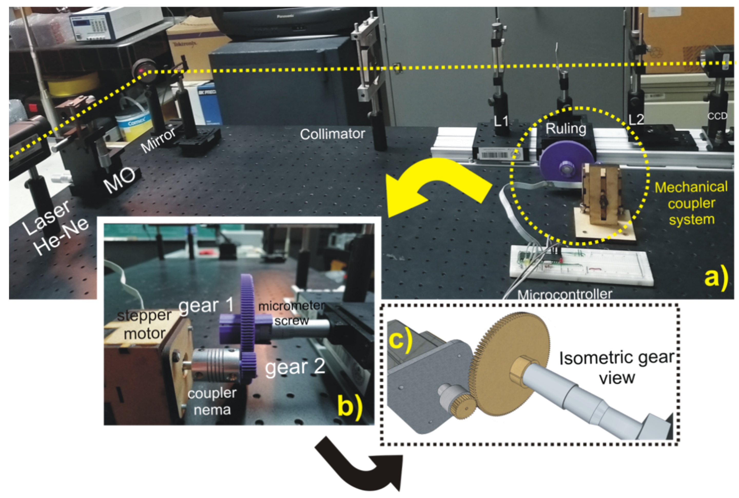
A microcontroller (PIC16F877A) receives codified instructions of the image capture and processing of the j^th interferogram from the LabVIEW platform. Then, the microcontroller, aided by a power stage, delivers the 4-bit impulse sequence required for a unipolar stepper motor (Nema17) operation (see Figure 3a). The stepper motor is coupled to a PLA 3D printed spur gear system to rotate a micrometric screw (Mitutoyo Head Series 149) of an optical translation stage, as it is shown in Figure 3b. The gear transmission produces a linear displacement of a Ronchi ruling with a period of $500 \mathrm{lines}/\mathrm{mm} \left(u_p=2 \mathsf{\mu }\mathrm{m}\right)$ mounted on the translation stage. In order to meet the interference condition in the object plane, the separation between the windows was set to $x_0=30 \mathrm{mm}$, considering a He–Ne laser with $\lambda =632.8 \mathrm{nm}$ and focal length $f=100 \mathrm{mm}$. The micrometer screw had a nominal resolution of $0.001$ inches per division $\left(25.4 \mathsf{\mu }\mathrm{m}\right)$, then, without a gear transmission system, a full turn is completed with a linear displacement of $0.025$ inches (635 µm). With a stepper motor resolution of $1.8°$, the ruling is transversally displaced 3.175 µm per motor step. According to Equation (2), the ruling displacement generates an aggregate phase of $\alpha =2\pi \left(3.175 \mathsf{\mu }\mathrm{m}\right)/2 \mathsf{\mu }\mathrm{m}\approx 10 \mathrm{rad}$ to the interference pattern, which exceeds the range of $\left(0,2\pi \right)$ in which the algorithms can calculate the phase. Therefore, a gear transmission system coupled to the micrometric screw allows the decreasing of the ruling linear displacement to meet the range from 0 to 2π rad. Figure 3c shows the designed 1:4 gear transmission system, which decreases the linear displacement of the ruling to $u_d=0.793 \mathsf{\mu }\mathrm{m}$, allowing theoretical phase shifts of $\alpha \approx 2.493$ rad.

It is worth mentioning that a commercially available piezoelectric optical translation system, which includes a driver and a coupling device, is approximately 1200% more expensive compared with our system based on a stepper motor system. Although a piezoelectric device can reach higher angular displacement resolution, our setup represents a reliable low-cost approach for real-time automatic phase recovery by phase shifting from a dual-aperture common-path interferometer.

Furthermore, the integration through a widely distributed platform, such as LabView, allows standard low-cost access to users interested in the proposed system.

Generally, phase-shifting techniques retrieve the object phase $\varphi \left(x,y\right)$ by solving an $N\times 3$ system of equations from equal phase steps and specific phase-shifter calibration [32]. Particularly, generalized phase-shifting interferometry (GPSI) does not require known and equal phase steps, however a specific phase-shifter calibration is required. As recently reported, self-calibration generalized phase-shifting interferometry (SGPSI) provides the possibility of unequal and unknown phase steps without the requirement of an exhaustive calibrating process to retrieve the object phase [26,27]. In this case, SGPSI advantages allow a straight forward calculation of the phase-step $\alpha$ introduced by linear displacement of the ruling. Digital grayscale pattern images are converted into an $m\times n$ matrix in order to apply the SGPSI technique and obtain the phase differences $\alpha$ between recorded interferograms using [27]:

$$\begin{array}{c}\cos \frac{1}{2}{\alpha }_1=\frac{\mathrm{tr}\left(q^{\mathrm{T}}r\right)}{\sqrt{\mathrm{tr}\left(q^{\mathrm{T}}q\right)\mathrm{tr}\left(r^{\mathrm{T}}r\right)}}\\ \cos \frac{1}{2}{\alpha }_2=\frac{\mathrm{tr}\left(p^{\mathrm{T}}q\right)}{\sqrt{\mathrm{tr}\left(p^{\mathrm{T}}p\right)\mathrm{tr}\left(q^{\mathrm{T}}q\right)}}\end{array}$$

(3)

$\mathrm{tr}(·)$ and ${(·)}^{\mathrm{T}}$ are the trace and transpose operators respectively; the restrictions are ${\alpha }_0=0,{\alpha }_1\in \left(0,{\alpha }_2\right)$ and ${\alpha }_2\in \left(0,2\pi \right)$, $p=I_0-I_1, q=I_1-I_2$, and $r=I_0-I_2$. Then, the phase of the probe arm $\varphi \left(x,y\right)$ is obtained by:

$$\tan \varphi =\frac{I_2-I_1+\left(I_0-I_2\right)\cos {\alpha }_1-\left(I_0-I_1\right)\cos {\alpha }_2}{\left(I_0-I_2\right)\sin {\alpha }_1-\left(I_0-I_1\right)\sin {\alpha }_2}$$

(4)

The block diagram of the SGPSI algorithm used to obtain $\varphi \left(x,y\right)$, including the automation, is shown in Figure 4. The automation of the phase retrieving by the proposed DACPI system was incorporated into the implementation in LabView, used for the capture of the interferograms. Equation (4) retrieves the original phase function, for this purpose the SGPSI requires a minimum of 3 phase-shifted interference patterns in order to achieve the values of ${\alpha }_j$. Each pattern is captured by a CCD camera from sequential motor steps, and then, converted into grayscale 2D $m\times n$ arrays: $I_0$, $I_1$, and $I_2$. The SGPSI algorithm is performed using the values of $p$, $q$, and $r$, obtained from the $I_0$, $I_1$, and $I_2$ interactions. Then, ${\alpha }_1$ and ${\alpha }_2$ are calculated (${\alpha }_0=0$). Next, the phase ${\varphi }_w$ is calculated, wrapped for a period $2\pi$ or integer multiples of $2\pi$, which leads to a discontinuous function in the solution. In this regard, several techniques known as unwrapping phase methods are used to eliminate such discontinuities to obtain a smoothed function of the phase by adding $2\pi$ or multiples of $2\pi$. LabView libraries includes the virtual instrument (VI) Unwrap Phase VI, which allows 1D phase unwrapping. In order to simplify the design of the algorithm, the VI was used and adapted for the 2D unwrapping of ${\varphi }_w$. The unwrapped phase $\varphi$ is then obtained.

4. Results and Discussion

Once the mechatronic system was implemented, computational tests were performed. The algorithm was proved using three simulated phase-shifted interference patterns labeled as (a), (b), and (c) in the LabView front panel, shown in Figure 5. The original function from the simulated phase steps of the interferograms was shown as reference in the plotting labeled as (e). Then, the proposed retrieving phase algorithm calculated the values of $p,q,r$ from the simulated interferograms to obtain the phase step values of $\alpha$.

Table 1. Comparison between the simulated and the calculated values for the phase shifts.

Simulated Value	Calculated Value	Error (Absolute Value)
${\alpha }_0=0$	${\alpha }_0=0$	-
${\alpha }_1=1.57079$	${\alpha }_1=1.586469$	0.015
${\alpha }_2=3.14159$	${\alpha }_2=3.142185$	0.0005

shows the comparison between the proposed and calculated phase step values ${\alpha }_1$ and ${\alpha }_2$ and the absolute value of the error. Next, the algorithm calculated the wrapped phase function ${\varphi }_w$, observed in the plot (d). Finally, the unwrapped phase ${\varphi }_u$ is obtained, as it is shown in the plot labeled as (f) in the front panel image, as it is displayed to the user. The plot (f) corresponds to the retrieved 2D unwrapped phase function obtained from the algorithm, which can be compared with the 2D original function of the plot (e). This comparison is shown in plot (g) as the subtraction (error) between them (red curve). Additionally, the plot labeled as (h) shows the calculated 3D phase function. As can be observed in Table 1, the non-zero error is attributed to the limitation of the used SPGSI algorithm, which required a high number of interference fringes to reduce the error [26]. In the proposed system, the error is considered acceptable due to its advantages compared with the reported systems. In our approach, the proposed SPGSI algorithm exhibited noise immunity which allowed the calculation of the phase from the experimental interferograms, avoiding undergoing filtering processes [33]. In addition, equal spacing displacement is not required from the obtained interferograms and the needless special calibration procedures.

Afterwards, experimental results were obtained. In order to generate the interference fringes, transparent acetate was used as the phase object placed in the probe window B of the object plane. It is worth noting that for experimental results, the angular displacements generated in each motor step are not equal. However, for the implemented algorithm, the equal steps condition is not mandatory since the SGPSI is capable of achieving phase shifts, even if these steps are unequal. Figure 6 shows a set of four CCD consecutive interference pattern captures. The images were arranged in two groups of three patterns. The first group, corresponding to the initial phase steps, includes the first three images whose intensities are $I_0$, $I_1$, and $I_2$. The second group stands for the new phase for each step calculation and includes the second, third and, fourth images with intensities $I_1$, $I_2$, and $I_3$. Then, the phase function ${\varphi }_w$ is obtained by calculating the values of ${\alpha }_1$ and ${\alpha }_2$ with the corresponding phase difference between each pair of interferograms.

As a result of evaluating the set of experimental patterns, the wrapped and unwrapped phase is calculated from the obtained phase steps for each motor step. Figure 7 shows the front panel of LabView for the implemented algorithm. The plots labeled as (a), (b), and (c) correspond to the calculated phase shift for each step. The plot (d) corresponds to the calculated wrapped phase. The 2D and 3D plots for the retrieved phase are labeled as (e) and (f), respectively. As it can be observed, by using three consecutive experimental patterns it is possible to automatically obtain the phase function, without reprocessing the data.

The results of the characterization of the phase shift introduced by each stepper motor rotation step are shown in Figure 8. The measurement was obtained from 47 consecutive experimental pattern captures. The calculated values of $\alpha$ from the consecutive images recorded were obtained by using the aforementioned algorithm. The first set of results was computed with the obtained interferograms from 1 to 3, the second set of results was computed with the obtained interferograms from 2 to 4, and so on to complete all 46 calculations of the phase step. The theoretical phase step value calculated with Equation (2) is ${\alpha }_T=2.493$ rad (blue line), whereas the average value of the experimental phase step of $\overline{\alpha }=2.483$ rad (green line) was obtained from the calculated values of $\alpha$ from the consecutive recorded interferograms. The bias between the theoretical and experimental values is $\left|{\alpha }_T-\alpha \right|=0.01$ rad. The average standard deviation of the total result is of $\sigma =0.197$. Finally, it is possible to calculate the average value with the uncertainty percentage as $\overline{\alpha }=2.483 \mathrm{rad}\pm 8\%$, which is comparable to the result obtained by manual transversal displacement of the ruling in a DACPI system but with measurements obtained over half a step of the reported values [29]. It is important to mention that because the algorithm is capable of evaluating phase changes with non-uniform shifts, the system was able to obtain the phase function with complex implementation, high-precision devices, and special calibration.

5. Conclusions

In this paper, we demonstrated the reliable operation of an automated DACPI system with real-time obtaining of the phase difference between the probe and reference windows. The phase extraction was achieved by a self-calibrated algorithm without the requirement of equally spaced displacements.

As a result of the experimental evaluation, it is demonstrated that the implementation of a real-time automatic system capable of transversely shifting a ruling to the optical axis in a dual-aperture common path interferometer is possible. The transverse displacement of the ruling generates a phase change between one interferogram and another, which the system is able to calculate using elements without requirement of extensive calibration. Additionally, the proposed system calculates the unwrapped phase and immediately displays it on a user-friendly platform, avoiding rework and increasing the precision compared to manually operated systems. From a set of 47 interferograms an average motor step phase difference of 2.483 rad was obtained, with a difference of 0.01 rad with respect to the theoretical value.

The proposed automated system is a reliable option to improve the accuracy when calculating the phase difference by using low–cost elements and a homemade ruling translation.