Variability of Gravel Pavement Roughness: An Analysis of the Impact on Vehicle Dynamic Response and Driving Comfort

Featured Application

In this article, we present a methodology for adapting pavement quality indexes for roads with gravel pavement. The findings presented in this article can be used to improve driving safety and gravel pavement maintenance.

Abstract

Gravel pavement has lower construction costs but poorer performance than asphalt surfaces on roads. It also emits dust and deforms under the impact of vehicle loads and ambient air factors; the resulting ripples and ruts constantly deepen, and therefore increase vehicle vibrations and fuel consumption, and reduce safe driving speed and comfort. In this study, existing pavement quality evaluation indexes are analysed, and a methodology for adapting them for roads with gravel pavement is proposed. We report the measured wave depth and length of gravel pavement profile using the straightedge method on a 160 m long road section at three stages of road utilization. The measured pavement elevation was processed according to ISO 8608, and the frequency response of a vehicle was investigated using simulations in MATLAB/Simulink. The international roughness index (IRI) analysis showed that a speed of 30–45 km/h instead of 80 km/h provided the objective results of the IRI calculation on the flexible pavement due to the decreasing velocity of a vehicle’s unsprung mass on a more deteriorated road pavement state. The influence of the corrugation phenomenon of gravel pavement was explored, identifying specific driving safety and comfort cases. Finally, an increase in the dynamic load coefficient (DLC) at a low speed of 30 km/h on the most deteriorated pavement and a high speed of 90 km/h on the middle-quality pavement demonstrated the demand for timely gravel pavement maintenance and the complicated prediction of a safe driving speed for drivers. The main relevant objectives of this study are the adaptation of a road roughness indicator to gravel pavement, including the evaluation of vehicle dynamic responses at different speeds and pavement deterioration states.

1. Introduction

Pavement surfaces for roads and urban streets are mostly made of concrete, asphalt, cobblestone, and gravel. The share of gravel pavement, particularly on local and regional roads of low- and middle-income countries, remains relatively significant. Decreased handling and comfort, the impact on roadside areas, and other destructive indicators from this point of view make global sustainable transportation hardly achievable [1]. The costs of gravel pavement construction are the lowest; however, its strength, environmental impact, and driving conditions are the poorest [2,3,4]. Gravel pavement must be maintained continuously by employing the blading technique to reduce transverse ripples and the resulting changes in surface elevation. It is also necessary to add bulk material periodically to gravel pavement due to the deterioration process. Rough gravel pavement increases fuel consumption and gas emissions [5], which is incompatible with mobility and life quality needs and environmental principles in today’s society. It is estimated that, based on a reference of 25 years, paving 1 km of gravel road results in 230,000 L of fuel saved and 580 tons of CO₂ emissions avoided [6]. Moreover, many road accidents occur on gravel roads with relatively high traffic volume [7]. Finally, safety, stability, and comfort systems including suspension development must also be adapted to operate efficiently under imperfect pavement with different degrees of roughness [8,9,10,11,12,13,14].

Currently, there are no straightforward methodologies for determining gravel road surface condition according to a driver’s need to travel safely and comfortably. The existing studies on vehicle response analyses, safety, durability, and fatigue loads are mostly related to paved roads [15,16,17,18]. Different indexes are used for road pavement quality evaluation; however, they are mainly used for asphalt or concrete pavements. One of the goals of this study is to analyse the existing indexes and develop a methodology for adapting such indexes to roads with gravel pavement. Instead of developing an original index, we proposed modifying one of the widely used indexes, thus, increasing the possibility of its further usage by operators responsible for ensuring road quality and by other researchers.

The goal is to develop the methodology for gravel road quality evaluation concerning pavement deterioration and vehicle dynamic response, providing appropriate maintenance indication for this pavement type.

This paper is organized into six sections, which includes the Introduction. In Section 2, related studies on road roughness are analysed, and the specificity of gravel pavement is provided. The impact of a gravel road on vehicle dynamic responses considering comfort, handling, and vehicle components’ degradation are taken into account. Road roughness measurement techniques and indexes used for quality evaluations are reviewed and the methodological gaps are identified. In Section 3, we provide the strategy for this study. In addition, we present the theoretical background for the selected index calculations. In Section 4, we describe the experimental procedure. In Section 5, the specificity of the international roughness index (IRI) approach for gravel pavement is analysed, and vehicle dynamic responses in the context of the excitation of sensitive frequencies at different driving speeds on gravel pavement are examined. In the Conclusions, we summarise the main results and explain how the IRI can be used for quality evaluation of gravel pavement and define future study guidelines.

2. Related Works

Three classes of grouped parameters of road pavement roughness, including geometric road parameters, statistical values, and performance-based indicators, are usually used in the literature [19]. Statistical parameters of geometric characteristics are directly related to the pavement texture profile’s geometry, which is described in the international standard ISO 13473-2 [20]. The performance indicators describe tyre–surface interaction, and this area is related to a broad scope of vehicle dynamic response.

Rapid changes in surface characteristics are one aspect of gravel pavement’s specific properties. The deterioration of gravel pavement is affected by climatic and meteorological factors such as wind, water, and temperature fluctuations. These factors alone, or in combination with vehicle loads, break down gravel pavement even faster. Thus, a five-level rating system has been introduced for evaluating the surface of gravel roads [21]. The system includes: (i) crown (shaping and grading quality); (ii) drainage (roadside ditches and culverts); (iii) gravel layer (thickness, gradation, particles shape and regularity, and gravel durability); (iv) surface deformation (corrugation, potholes, and ruts); (v) surface defects (dust and loose aggregate particles). Deteriorated pavement with specific waves of a narrow band spectrum is partly similar to rigid pavement that contains a high number of cosine shape obstacles. In such a case, the road profile is considered to be quasi-homogeneous, i.e., standard profile processing is not directly applicable [22].

The corrugation or ‘washboard’ phenomenon of gravel pavement occurs in small transverse ripples. The periodic vertical motion of a vehicle’s wheels, which is caused by suspension characteristics and body bounce, affects harmonic loads and ripple formation. Very small and initially insignificant imperfections primarily cause corrugation on an unpaved road, such as small undulations, variance in surface flexibility, or even sporadic grains [23,24]. Following a study on the factors causing gravel road corrugation, a regression analysis enabled the researchers to define the extent of corrugation [25]. Surface deformation, especially corrugation, is usual for dirt roads under dry weather conditions; however, ripples also occur on paved surfaces where vehicle traffic involves intensive braking or acceleration, which are typical in vertical curves of roads near intersections.

The process of decomposition and overall deterioration of quality is more difficult to characterize for gravel pavement than asphalt, concrete, or cobble road pavements. During periods of dry weather, due to the interaction between wheels and road surface, pavement wear increases roads’ dustiness, and thus, negatively impacts the comfort and health of vehicle occupants accessing and using this particular type of road [26,27]. On the contrary, rain washes away materials used for reducing dustiness as well as fine particles from the pavement surface, weakening the bedrock and resulting in an increased number of defects and deeper tracks in gravel pavements [28].

Defects in gravel pavement have been shown to result in a decrease in driving speed, comfort, and friction [29,30], as well as an increase in vehicle chassis damage [31]. Wavelength and the spatial frequency of road pavement characterise irregularities and a texture effect on vehicle dynamic response. Wear on vehicle components, rolling resistance, and discomfort properties are sensitive to longer wavelengths (unevenness and partly mega-texture), while friction between tyres and the road interacts at mega-, macro-, and micro-texture levels. Moreover, two types of pavement profile wave sizes have been specified in the tyre-asphalt contact area: short waves are 3–6 mm in length and long waves are 20–30 mm [32]. This particular study demonstrated that the maximum height of 1 mm micro-irregularities were found until adhesion tended to increase; however, this regularity was not applicable for rough surfaces.

Different maintenance procedures are applied to gravel pavement which mainly include light or hard blading, sand cushioning, reshaping, regravelling, etc. [33]. Bitumen emulsion spraying is used as an effective method for decreasing dustiness [34]. Jurkevičius et al. [35] defined a road maintenance management system based on a model for predicting pavement performance and deterioration. The model could be applied for gravel pavement and calculated the loss of gravel thickness [36], therefore, applicable for planning the thickness of gravel layer for road rehabilitation or a new road. Data on traffic, climate, and roughness variation; material quality; gradeability; and cost should be collected to select an optimal road maintenance strategy.

Pavement quality evaluations that include roughness measurements are necessary for planning road pavement maintenance. Various methods and devices have been used for evaluating the roughness and deterioration level of road pavement [37,38]. For profiling, various devices such as a straightedge, a dipstick, the Merlin machine, and an inertial profiler have commonly been used [39,40]. Response-based devices (displacement or acceleration sensors, equipped trailers, or vehicles) are widely applied due to fast processing and low-cost equipment availability [41,42,43,44,45,46,47]. Monitoring the state and quality of unpaved roads can be based on visual observations and in-person surveying, contrary to paved road evaluations in which data are collected automatically [48]. A digital image acquisition system has been applied utilizing an unmanned aerial vehicle (UAV); however, limited pavement distresses were captured (mainly potholes and rutting) and the flight range of the UAV made not widely applicable. A ride quality assessment of vehicle response is convenient enough, although the most characteristic driving speed is not the same for different quality pavements. Various identification principles are also known from studies in the literature, for example, a mechanical profilometer for three-dimensional terrain models [49], smartphone accelerometer processing [50], digital image analysis [51], and reconstruction methods using additional sensors [52,53].

Various ride quality assessment indicators have been defined to describe the impact of road roughness and, in the last 15 years, several new indexes have been introduced [54]. Loprencipe and Zoccali [55] compared the relations among Ride Number (RN), Michigan Ride Quality Index (RQI_Mich), Minnesota Ride Quality Index (RQI_Mn), and frequency-weighted vertical acceleration ($a_{wz}$) and their relationships with the most-used IRI. The RN, RQI_Mich, and RQI_Mn were developed considering road customer opinions, and their thresholds of ride quality level were not speed related. Therefore, the weighted acceleration $a_{wz}$ provided by ISO 2631 [56] was applicable for lower speed roads (not exceeding 50 km/h). Gurmail and Kiss [57] analysed the response of towed vehicles employing the power spectral density (PSD) function to determine the effect of vehicle wheel–ground interaction on structural deterioration. Different types of roads with high- and low-quality surfaces were selected for the simulation analysis. The same frequency ranges with the elevated local maximum of the PSD characteristic increasing speeds from 3.6 to 18 km/h were determined for a rough gravel road. This study also stated that, under low speed, towed vehicle conditions (up to 20 km/h), micro-obstacles (humps and holes) occurred with shorter than 2.4 m of wavelength or greater than 0.4–1 m wave numbers on agricultural roads. A smooth exponential increase in root mean square (RMS) values of measured accelerations in a speed range from 3.6 to 25 km/h was determined. Lower-quality road surfaces with irregular forms of roughness are not suitable for the conventional IRI-based description, despite its broad applicability and simple enough computational implementation [58]. Different values of other indicators (for passengers in particular) were determined for roads with the same IRI values; therefore, alternative roughness or vehicle/passenger response indicators (such as the RMS value of acceleration) could be used for specific pavements. Some significant aspects of comfort evaluation in the cabins of different bus topologies were also highlighted as an IRI limitation [59]. First, it was argued that, in the case of similar IRI values, it was possible that there could be three different road profiles and that passengers would experience different vibration conditions. Then, insufficient sensitivity to lateral motions (acceleration) was proven based on experimental data. Due to the limited IRI evaluation of specific or unpaved road surfaces, dynamic response-based devices or road profile scanners have been used [45]. Devices added onto a vehicle have shown a high enough correlation with the IRI and allowed real-time measurements. However, evaluations of different roughness indicators have shown that nearly all the roughness measuring devices employed around the world could produce measurements on the same scale, as long as that scale was suitably selected; therefore, the IRI was defined [60,61]. The World Bank developed an IRI after conducting the International Road Roughness Experiment (IRRE) in Brazil in 1982. The aim of the experiment was to harmonise the existing indices for evaluating pavement roughness. Due to its stability over time and transferability over the world, it has become the most widely employed pavement index (not only for roughness assessment) in developed countries [62,63,64,65] and in developing countries [66,67,68]. Therefore, it is preferable to adopt an existing and known index to gravel roads instead of developing a new one.

Road infrastructure in different regions has been developed unevenly as there are various gravel coatings in suburban and rural areas. The majority of studies on vehicle–road interaction have focused on asphalt pavement. Evaluations of gravel road conditions have commonly been performed using methodologies developed several decades ago, and therefore new solutions are needed.

3. Indexes for Gravel Road Quality Assessment

The fundamental concept of road surface profiles at different mechanical vibration levels is described by the international standard ISO 8608 [69]. The PSD of vertical road profile displacement, $G_d\left(n\right)$, or its rate of change by velocity, $G_v\left(n\right)$, or acceleration, $G_a\left(n\right)$, conforming to spatial frequency, $\left(n\right),$ are used for defining the degree of roughness:

$$G_d\left(n\right)=G_d\left(n_0\right){\left(\frac{n}{n_0}\right)}^{-w},$$

(1)

$$G_v\left(n\right)={\left(2\pi n\right)}^2·G_d\left(n\right),$$

(2)

$$G_a\left(n\right)={\left(2\pi n\right)}^4·G_d\left(n\right),$$

(3)

where $n$ is the spatial frequency (cycles/m); $n_0$ is the reference spatial frequency (0.1 cycles/m); $w$ is the pavement waviness indicator, or the exponent of the fitted PSD. For general use, the road roughness indicator usually takes the values of 1.75 < $w$ < 2.25 [70] and for ISO classification assuming constant velocity PSD, $w$ = 2.

The profile of gravel pavement cannot be approximated with the waviness of w = 2 used in ISO 8608, which usually occurs on paved roads [46]. Múčka [71] reported that up to 40% of roads had differences in wavebands, and 20% of tested sections had short wave unevenness ($w$ > 2). Another type of specific road usually used for evaluating vehicle dynamic response, known as Belgian paving, also has few brakes in its displacement spectral density characteristic [72]. There, the wavenumber of 6 cycles/meter corresponds with the size of cobbles forming the pavement [73].

Generally, PSD expresses power in a signal per unit frequency [74]. The PSD of road profile displacement can also be expressed by an unevenness index $C$ [75]:

$$G_d\left(n\right)=C·n^{-w}.$$

(4)

Wavelength λ (m) has an inverse value of spatial frequency. In the time domain, frequency is expressed as the ratio between wavelength and vehicle speed $v$ (m/s), which generally satisfies conditions for light vehicles [76,77]:

$$0.5 \mathrm{Hz}<\frac{v}{\lambda }<15 \mathrm{Hz}$$

(5)

In the context of vehicle dynamic response and vibration response analysis, it is more convenient to convert excitation from road pavement spatial frequency $n$ (cycles per meter) to temporal frequency $f$(cycles per second or Hz). In this case, the supposed vehicle speed (v) is involved [78]:

$$f=n·v.$$

(6)

Then, the PSD of the road pavement, in consonance to temporal frequency $G_d\left(f\right)$, is adapted to vehicle speed:

$$G_d\left(f\right)=\frac{G_d\left(n\right)}{v}.$$

(7)

The IRI is the most frequently used single-number indicator usually implemented in road maintenance management plans, ride comfort, or stability assessments. The IRI value is estimated from the reference quarter car model (Figure 1a), also known as the Golden car model [39], driving at 80 km/h. The highest sensitivity for IRI computation was found from 0.065 to 0.42 cycles/m (wavelength from 15 to 2.4 m) (Figure 1b), which also varied from the selected sample interval and integration method [79]. The general IRI computation is based on two components as the velocity of suspension displacement [79,80]:

$$\mathrm{IRI}=\frac{1}{L}{{\displaystyle \int }}_0^{L/v}\left|{\dot{z}}_{sm}-{\dot{z}}_{usm}\right|dt,$$

(8)

where $L$ is the length of the evaluated road profile (m), $v$ is the longitudinal vehicle speed applied for the quarter car model (m/s), ${\dot{z}}_{sm}$ is the the velocity of sprung mass (SM) vertical displacement (m/s), ${\dot{z}}_{usm}$ is the the velocity of unsprung mass (USM) vertical displacement (m/s), and $dt$ is the time increment (s).

The dynamic load coefficient (DLC) has been used for evaluating vehicle response to ride safety and driving stability. It shows variations in the vertical tyre force as compared with its static force [81,82]:

$$\mathrm{DLC}=\frac{{\mathrm{RMS}}_{Fz,\mathrm{dyn}}}{F_{\mathrm{stat}}},$$

(9)

where $F_{\mathrm{stat}}$ is the static force and ${\mathrm{RMS}}_{Fz,\mathrm{dyn}}$ is the the root mean square of the dynamic vertical tyre force ($F_{z,\mathrm{dyn}}$), determined by applying a vehicle model simulation or using the formula:

$$F_{z,\mathrm{dyn}}=k_t\left(z_{usm}-h\right),$$

(10)

where $k_t$ is the tyre radial stiffness (taken from the Golden car model), $z_{usm}$ is the vertical displacement of USM, and $h$ is the vertical roughness of the road pavement.

The DLC value usually ranges from 0.05 to 0.3, and ride safety is high when DLC < 0.1. In contrast, a value above 0.15 is related to shaking wheel interaction with the rough pavement and an increase in contact loss [83].

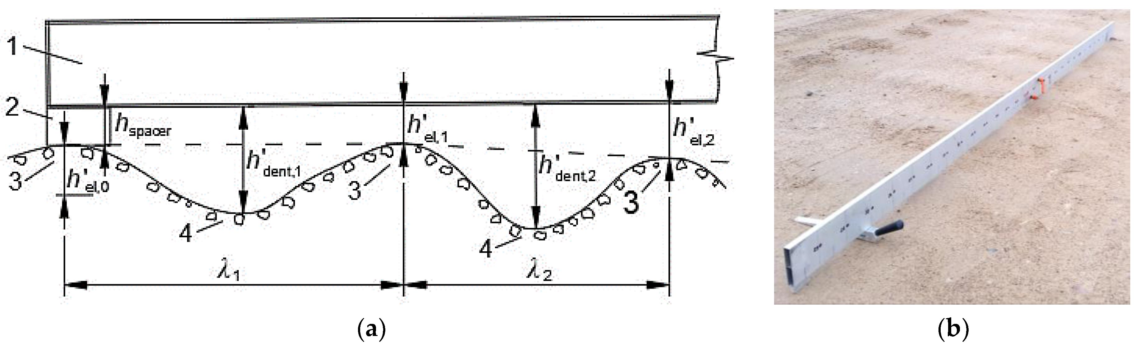
4. Roughness Measurement Using a Straightedge

The straightedge method for the pavement rut depth measurement [84] was selected for the data collection from the real gravel pavement. The proposed static method is based on measuring the gap between the road surface and a constant length (3.0 m) beam placed along the track corresponding to a vehicle’s left-side wheels. In this study, the straightedge method for measuring gravel pavement longitudinal roughness was adopted, which is usually characterised by higher roughness. Therefore, a small correction in measurement was made by adding 20 mm height spacers ($h_{\mathrm{spacer}}$) at the ends of the beam (Figure 2). An additional spacer was used in the cases when the end of the beam was over pavement dent.

The actual height of elevation and dent is determined by subtracting added spacer height (20 mm) considering each measured vertical distance, which is the clearance between the bottom of the straightedge and the pavement surface at corresponding elevation and dent:

$$h_{\mathrm{el}}=h{\prime }_{\mathrm{el}}-20,$$

(11)

$$h_{\mathrm{dent}}=h{\prime }_{\mathrm{dent}}-20,$$

(12)

where $h{\prime }_{\mathrm{el}}$ and $h{\prime }_{\mathrm{dent}}$ are the measured height of elevation and dent, respectively (mm); $h_{\mathrm{el}}$ is the actual height of elevation or clearance between the bottom of the straightedge and the pavement at corresponding elevation (mm); $h_{\mathrm{dent}}$ is the actual depth of dent or clearance between the bottom of the straightedge and the pavement at corresponding dent (mm).

The first stage of data post-processing included the inversion of data on the measured pavement elevation. Thus, the negative values of pavement dent were obtained. The absolute depth (amplitude) of the first wave ${\Delta }_{{\lambda }_1}$ (Figure 2), meaning the difference between dent depth and the average of neighbouring elevations, is expressed by the formula:

$${\Delta }_{{\lambda }_1}=h_{\mathrm{dent},1}-\frac{h_{\mathrm{el},0}+h_{\mathrm{el},1}}{2}.$$

(13)

The absolute depth (amplitude) of the second and next waves are as follows:

$$\begin{gathered} {\Delta }_{{\lambda }_2}=h_{\mathrm{dent},2}-\frac{h_{\mathrm{el},1}+h_{\mathrm{el},2}}{2}, \\ ⋮ \\ {\Delta }_{{\lambda }_N}=h_{\mathrm{dent},N}-\frac{h_{\mathrm{el},N-1}+h_{\mathrm{el},N}}{2}. \end{gathered}$$

(14)

A straight section of rural road, 160 m in length, with gravel pavement was selected for this study. Pavement roughness was measured considering the different states of the pavement. The first state (Pavement State 1, PS-1) means that the gravel pavement measurement was carried out two days after pavement maintenance using the blading technique without adding gravel material to the existing road surface. This state corresponds to the best-expected quality and driving conditions. The second state (Pavement State 2, PS-2) is described as a middle-quality gravel road, three weeks after pavement maintenance and the start of intensive road deterioration. The third state (Pavement State 3, PS-3) corresponds to the worst pavement quality, when maintenance is expected.

After blading, large grains were observed on the gravel’s flat surface; however, it did not have a significant influence on vehicle response because of tyre enveloping properties. The formed ripples were noticeable on the surface before maintenance (worst condition), and almost no individual free grains were found.

5. Results

The processed data on the measured profile elevation conforming to the pavement state of the road section are shown in Figure 3. The amplitudes do not exceed the elevation value of 20 mm in all pavement states; however, the profiles have noticeable differences which are described further.

The determined surface roughness of the analysed road section is presented in line with ISO 8608 methodology in the form of displacement spectral density—spatial frequency (Figure 4). The pavement roughness description concerning the PSD log-log plot has a specific break from a smooth characteristic at spatial frequency $n$ = 2 cycles/m (Figure 4).

The characteristic of PS-3 has an additional break at around 6.5 cycles/m. The characteristic PSD slope changes show variations in profile waviness at different bands of waves (long, medium, or short). The corrugation or ‘washboard’ phenomenon is recognised at the investigated road section. It is the most characteristic for the PS-3 state, where the shortest waves with the smallest variance are established. Furthermore, the maximum number of the estimated waves represented PS-3, which confirmed the worst pavement quality. Such smooth and constant ripples at certain road sections make driving extremely uncomfortable and unsafe at a specific speed, which is also one of the reasons for pavement corrugation. The results of the performed analysis of the wavelengths formed on the gravel pavement were used to study the reliability of the calculated IRI of the investigated pavement.

5.1. The IRI Approach for Gravel Pavement

Methodically, the velocities of SM and USM in a vertical direction of the Golden car model are determined and used for calculating the IRI value (Equation (8)). The second column in

Table 1. The estimated IRI values of the analysed gravel pavement.

Pavement State	IRI, m/km	Velocity RMS, m/s
		SM	USM
PS-1	6.33	0.0283	0.1821
PS-2	7.28	0.0313	0.2303
PS-3	5.51	0.0378	0.1530

shows the IRI values of the different states of the gravel pavement at a driving speed of 80 km/h, as provided in the ASTM [80]. Under the deteriorating road pavement condition, the IRI values change inconsistently; the highest IRI value (7.28 m/km) is obtained under PS-2 condition, while the lowest IRI value (5.51 m/km) is obtained under PS-3 condition. This is not in line with the visually observed (Figure 3) trends of pavement roughness deterioration from PS-1 to PS-3. To analyse the resulting distribution of IRI values concerning pavement condition, the vertical velocities of SM and USM were calculated. Table 1 shows the calculated RMS values of the SM and USM velocities in vertical directions. The RMS is calculated as follows:

$${\mathrm{RMS}}_{{\dot{z}}_i}={[\frac{1}{T}{{\displaystyle \int }}_0^T{\dot{z}}_i{}^2 dt]}^{1/2},$$

(15)

where $T$ is the duration of the evaluated road profile (s) and $i$ is the indicator for the SM or USM depending on the calculated parameter (${\dot{z}}_{sm}$ or ${\dot{z}}_{usm}$).

The values presented in Table 1 show that the RMS of the SM velocity increases along with consistent deterioration of the road pavement condition (from PS-1 to PS-3), but the RMS value of the USM velocity is unevenly distributed (such as the IRI values). The SM movement is inhibited by suspension elements (mainly dampers). At the same time, the USM interacts with the gravel pavement through the tyres, for which stiffness ($k_t$) is around ten times higher than that of suspension ($k_s$). As a result, the USM moves faster than the SM and has a more significant effect on calculating the IRI. These results indicate that the calculated IRI values are not suitable for analysing gravel pavements in which the wavelengths of the dominant length in the mega-texture area are formed. Similar results of higher sensitivity of wheel holder vibrations to the IRI value as compared with vehicle frame vibrations have been captured following measurements of reconstructed urban roads with cobblestone and asphalt pavements in [85].

The IRI values of the gravel pavement are determined by simulating a quarter car model as a vehicle moving at a speed of 80 km/h. Due to comfort and sufficient stability, the tested road section of gravel pavement is characterised by lower driving speeds. Therefore, the IRI values were calculated for a broader (30–90 km/h) speed range (Figure 5a). The received IRI values are significantly higher at lower speeds because the same road section is covered over a longer time duration, leading to higher accumulated suspension displacement in the IRI calculation. In this case, the distribution value at a given speed under a certain gravel pavement condition rather than the IRI absolute value is analysed. Figure 5a shows that, at lower speeds (30 and 40 km/h), the IRI values increase along with road pavement deterioration from PS-1 to PS-3. At speeds above 45 km/h, the distribution of the IRI values changes; the values of IRI_PS-3 corresponding to the worst gravel pavement condition become lower than the values of IRI_PS-2, whereas, at speeds above 55 km/h, the values of IR_{IPS 3} are the same as the worst gravel pavement condition and become lower than that of IR_IPS-1 (under the best-quality gravel pavement state). Thus, for calculating the IRI value, a speed of 45–55 km/h meets the transition phase, the IRI value of which is incorrectly consistent with the pavement condition.

The RMS of the SM and USM velocities was used to analyse variations in the IRI values (Figure 5b). Fluctuations in the RMS values demonstrated that an increase in driving speed resulted in minor changes in the SM velocity (continuous lines). However, changes in the velocity of the USM were found to be significant (dotted lines). In addition, USM_PS-3 is on a declining trend as speed increases while USM_PS-1 and USM_PS-2 are on an upward trend. These trends in the USM are repeated for IRI values and confirm that a speed of 30–45 km/h is compatible with the pavement state (PS) of the gravel road (Figure 5a).

5.2. Vehicle Response to the Pavement Surface State

In line with ISO 8608, the presented initial characteristic of the measured road roughness (Figure 4) shows a clear peak of displacement PSD at a spatial frequency of 2 cycles/m for the third pavement surface (PS-3) state. This peak is also repeated at six cycles/m of the frequency range. Such unevenness of the characteristic is considerably weakened in the second pavement surface (PS-2) state and is completely invisible under the best pavement surface (PS-1) state. Converting road roughness characteristics to temporal frequency (Equations (6) and (7)) reveals these characteristics’ irregularities at different vehicle driving speeds (Figure 6). Speeds up to 70 km/h, shown as higher road speeds on the gravel pavement, are prohibited under national road traffic regulations [86]. The most pronounced fractures in the elevated PSD are observed for the third pavement surface PS-3 state (Figure 6): a peak for 10 km/h at 5–6 Hz, a peak for 30 km/h at 15–18 Hz, a peak for 50 km/h at 23–30 Hz, and a peak for 70 km/h at 33–42 Hz.

Driving at lower speeds (10–30 km/h) through short wavelength roughness (PS-3) formed on the gravel pavement (macro-texture level) demonstrates that vibration frequency caused by waves approaches the natural frequency of vehicle USM (11–15 Hz). This order vibration tends to increase the variability in the normal load of the wheel described by the DLC [87,88]. The normal force of the tyre depends on suspension characteristics [89]; however, road pavement and driving speed have a direct influence. The calculated DLC values for the quarter car model working at a broad speed range (10–90 km/h) are shown in Figure 7. Here, the Golden car model simulation in the MATLAB/Simulink environment was used. Conforming to the pavement surface state, the obtained DLC values have the same distribution as the IRI (Table 1) due to the dominant movement of the USM (the highest RMS of the USM for PS-2). Both tendencies (IRI and DLC) prove that the second pavement surface (PS-2) state excites resonant motion for the analysed light car model.

To analyse vehicle response changes in different gravel pavement surface states, the spectral density of pavement displacement at a vehicle vertical dynamics sensitive range of 0–20 Hz was selected (Figure 8). The excitation of the road pavement to the vehicle driven at a speed of 10 km/h corresponds to an increase in pavement deterioration level (Figure 8a). Although there is no significant rise in pavement excitation for the SM and USM dynamics at 10 km/h (at 1–2 Hz and 10–14 Hz, respectively), the undesired excitation occurs at a human body sensitive frequency range of 4–8 Hz (ISO 2631-1) on PS-3 and PS-2 states. Since a speed of 10 km/h is more typical for a special purpose vehicle with different suspension and tyre properties, in this study on light vehicle application, we continued analysing higher speeds.

The characteristic of 30 km/h (Figure 8b) highlights two crucial cases. Excitation at a human body sensitive frequency range of 2.5–5.5 Hz is higher in the middle-quality pavement state (PS-2) and is the lowest in the PS-3 state. This also shows that a slightly higher driving speed (from 10 km/h) makes a milder impact on the human body. The second important point, in the case of 30 km/h, indicates the exclusively high excitation of the PS-3 state at a frequency range of 10–18 Hz. This frequency range covers the resonant frequency of the USM and increases variability in dynamic tyre force, contact loss, and vehicle chassis wear. The corresponding peak of the DLC characteristic is marked with a dotted line in Figure 7. The conversion of PS-3 characteristics from the lowest position at 2.5–5.5 Hz to the highest at 10–18 Hz (Figure 8b) shows possible erroneous driver’s sensations about comfortable enough driving, but an imperceptible decrease in road holding.

The characteristics of 50 km/h and 70 km/h do not have distinguished peaks or rises (Figure 8c,d); however, the two characteristics have the same feature of higher PS-2 excitation in the middle-frequency range, i.e., 4–9 Hz for 50 km/h and 5.5–12.5 Hz for 70 km/h. The difference between these two cases is that excitation corresponding to 50 km/h affects the human body, while excitation corresponding to 70 km/h additionally affects USM dynamics (wheel contact). The latter is also recognised as a DLC characteristic (marked with the continuous line in Figure 7).

The excitation at a low-frequency range of 1–2 Hz sensitive for driving comfort is higher on the PS-3 state, but this is reasonable because it is the worst pavement quality.

In general, all PSD curves of pavement excitation tend to descend with each increase (Figure 8). This may lead to a false perception that a higher speed on the gravel pavement gives better driving comfort or safety. The individual analysis of different operating frequencies made it possible to distinguish vehicle stability, comfort, and human body sense. Lower pavement excitation for specific frequencies causes better comfort, but the individual cases of a high DLC warn about the potential of vehicle stability loss.

Natural frequencies utilising the quarter car model’s damping ratios (Golden car parameters [39]) were determined from the Bode plot (Figure 9a). Natural frequencies were placed into the speed-wavelength-frequency characteristic (Figure 9b), showing sensitive frequencies overlapping pavement wavelengths at a specific driving speed. The characteristic shows that SM (vehicle body) vibrations are amplified by the pavement with the dominant wavelength of 2–30 m at a driving speed in the range of 10–130 km/h, while USM vibrations (wheels and axles) are amplified by the wavelengths of 0.25–3.5 m in length (Figure 9b).

For example, normal highway asphalt pavement with an unevenness of 10 m wavelength causes uncomfortable driving at around 30–50 km/h (speed curves cross the solid black line in Figure 9b). However, this speed is not characteristic of highway driving, and thus a hardly deteriorated pavement prevents discomfort. Vehicle instability caused by wheel resonance under such conditions is barely activated as the natural frequency of the USM (wheel hop) does not cross any speed curve at the above mentioned 10 m wavelength. On the contrary, the second example presents unpaved roads with gravel pavement where short wavelengths dominate. Considering the 1 m wavelength, the natural frequency of SM is not reached (solid line in Figure 9b). However, the USM resonances at a speed range of 30–50 km/h (crosses dotted line), thus, causing unstable wheel contact with the pavement. Shorter wavelengths activate USM resonance at a lower driving speed. Furthermore, the human body sensitive frequency range of 4–8 Hz falls into the short-middle wavelength band (0.3–5 m) for a wide range of speeds. The obtained vibrations correspond to uncomfortable and unstable driving at a specific road pavement waviness for a certain speed.

In this Section, it was proven that the IRI index could be used to evaluate gravel road conditions; the significance of the proposal for calculating the index using the specific velocity interval from 30 to 45 km/h for gravel pavement was indicated. The PSD and DLC indexes with frequency response characteristics provide valuable information about the impact of different road roughness levels on discomfort and safety at a certain driving speed.

6. Conclusions

In this study, we aimed to determine changes in the quality of gravel pavement overtime during the service life of a road, in line with the level of surface roughness and pavement excitation on vehicle response and driving comfort. The roughness of the experimental 160 m section of road with gravel pavement was measured continuously three times by adopting the 3 m straightedge method: (1) two days after pavement maintenance (blading), (2) three weeks after pavement maintenance, and (3) assessing the worst pavement quality before maintenance. The measurement results showed that the road quality continuously deteriorated with an increase in pavement roughness. Pavement elevation spectral density disclosed several fractures in the roughness log-log plot, which meant variations in pavement waviness. For the worst pavement quality (PS-3), a dominance of short waves of approximately 0.5 m in length was found (lowest standard deviation), which was compatible with the corrugation phenomenon of the transverse ripples formed. Furthermore, such a wavy pattern was found to cause unsprung mass (USM) resonant excitation of the vehicle before the worst road quality was achieved.

Spatial frequency conversion to temporal was done to analyse vehicle dynamic responses at different driving speeds. Although the specific fractures of surface power spectral density (PSD) characteristics remained, for the worst pavement quality state, in particular, the speed-affected frequencies shifted to higher bands. Speed is mostly related to driving safety, and therefore the dynamic load coefficient (DLC), as the indicator of tyre–pavement interaction and vehicle stability, was determined considering the analysed pavement states. Even quarter car simulations of driving at a low speed (<30 km/h) showed that the DLC reached values higher than 0.15 but did not exceed 0.3 when the proportion of wheel contact loss increased rapidly. However, the DLC undesirably increases at a low speed of 30 km/h on the worst pavement quality and a high speed of 90 km/h on the middle-quality pavement. Even though most countries have a speed limit of 70 km/h on gravel pavement, the potential wheel contact force loss draws attention to timely road maintenance. Variations in driving comfort sensation and the indirect prediction of wheel–pavement interaction complicate a driver’s selection of safe driving speed. Therefore, vehicle active chassis systems should be continuously developed for better performance on a specific road such as variable roughness gravel pavement.

In consonance with the estimated vehicle suspension response to the investigated type of gravel pavement, IRI values have been found to rarely correspond to the actual level of pavement roughness. Therefore, this worldwide single-number indicator used for road maintenance planning is not appropriate for unpaved pavements with unsteady waviness. Absolute IRI values do not provide reliable results that can be used for safe speed estimation. However, calculating the IRI at a speed range of 30–45 km/h shows an increase in the values corresponding to the deteriorating pavement state. Thus, the IRI values calculated at a low speed (30 km/h) are suitable for assessing gravel pavement condition and road maintenance planning.

The achieved results can be used to assist operators responsible for ensuring road quality and for decision making about road maintenance, to analyse the effects of unpaved roads on vehicle driving stability and comfort, and to support the performance of active safety systems, drivers, road maintenance planners, and road supervisors.

Future experimental and theoretical studies should focus on vehicle dynamic response measurements and driver comfort evaluation in different driving modes under varying pavement states. Continuous research should also investigate higher-order frequency bands related to the issues of tyre dynamics and active vehicle safety control while driving on unpaved roads. The development of pavement roughness measurement utilising laser sensors and artificial intelligence-based image analysis for pavement state identification is planned. The results of direct roughness measurements and their analysis presented in this study could also be used for validating the results of further research.

References

1. Horiuchi, S.; Tsuda, A.; Kobayashi, H.; Redding, C.A.; Prochaska, J.O. Sustainable transportation pros, cons, and self-efficacy as predictors of 6-month stage transitions in a Chinese sample. J. Transp. Health 2017, 6, 481–489. [Google Scholar] [CrossRef]
2. Obeng, D.A.; Tuffour, Y.A. Prospects of alternative funding sourcing for maintenance of road networks in developing countries. Transp. Res. Interdiscip. Perspect. 2020, 8, 100225. [Google Scholar] [CrossRef]
3. Pasindu, H.R.; Gamage, D.E.; Bandara, J.M.S.J. Framework for selecting pavement type for low volume roads. Transp. Res. Proc. 2020, 48, 3924–3938. [Google Scholar] [CrossRef]
4. Petkevičius, K.; Maskeliūnaitė, L.; Sivilevičius, H. Determining travel conditions on motorways for automobile transport based on the case study for Lithuanian highways. Transport 2019, 34, 89–102. [Google Scholar] [CrossRef] [Green Version]
5. Ziyadi, M.; Ozer, H.; Kang, S.; Al-Qadi, I.L. Vehicle energy consumption and an environmental impact calculation model for the transportation infrastructure systems. J. Clean Prod. 2018, 174, 424–436. [Google Scholar] [CrossRef]
6. Gleave, S.D.; Frisoni, R.; Dionori, F.; Casullo, L.; Vollath, C.; Devenish, L.; Spano, F.; Sawicki, T.; Carl, S.; Lidia, R.; et al. EU Road Surfaces: Economic and Safety Impact of the Lack of Regular Road Maintenance. European Parliament—Directorate General for Internal Policies, Policy Department B: Structural and Cohesion Policies, Transport and Tourism. 2014. Available online: https://www.europarl.europa.eu/RegData/etudes/STUD/2014/529059/IPOL_STU(2014)529059_EN.pdf (accessed on 16 August 2021).
7. Mamčic, S.; Sivilevičius, H. The analysis of traffic accidents on Lithuanian regional gravel roads. Transport 2013, 28, 108–115. [Google Scholar] [CrossRef]
8. Pretagostini, F.; Ferranti, L.; Berardo, G.; Ivanov, V.; Shyrokau, B. Survey on Wheel Slip Control Design Strategies, Evaluation and Application to Antilock Braking Systems. IEEE Access 2020, 8, 10951–10970. [Google Scholar] [CrossRef]
9. Van der Merwe, N.A.; Els, P.S.; Žuraulis, V. ABS braking on rough terrain. J. Terramech. 2018, 80, 49–57. [Google Scholar] [CrossRef] [Green Version]
10. Cao, D.; Song, X.; Ahmadian, M. Editors’ perspectives: Road vehicle suspension design, dynamics, and control. Veh. Syst. Dyn. 2011, 49, 3–28. [Google Scholar] [CrossRef] [Green Version]
11. Hamersma, H.A.; Els, P.S. Improving the braking performance of a vehicle with ABS and a semi-active suspension system on a rough road. J. Terramech. 2014, 56, 91–101. [Google Scholar] [CrossRef] [Green Version]
12. Šabanovič, E.; Žuraulis, V.; Prentkovskis, O.; Skrickij, V. Identification of Road-Surface Type Using Deep Neural Networks for Friction Coefficient Estimation. Sensors 2020, 20, 612. [Google Scholar] [CrossRef] [Green Version]
13. Žuraulis, V.; Surblys, V.; Šabanovič, E. Technological measures of forefront road identification for vehicle comfort and safety improvement. Transport 2019, 34, 363–372. [Google Scholar] [CrossRef] [Green Version]
14. Savitski, D.; Ivanov, V.; Shyrokau, B.; De Smet, J.; Theunissen, J. Experimental study on continuous ABS operation in pure regenerative mode for full electric vehicle. SAE Int. J. Passeng. Cars Mech. Syst. 2015, 8, 364–369. [Google Scholar] [CrossRef]
15. Gao, H.; Jézéquel, L.; Cabrol, E.; Vitry, B. Chassis durability and comfort trade-off at early stage of project by virtual proving ground simulation. Veh. Syst. Dyn. 2021, 5–20. [Google Scholar] [CrossRef]
16. Fauriat, W.; Mattrand, C.; Gayton, N.; Bekou, A.; Cembrzynski, T. Estimation of road profile variability from measured vehicle responses. Veh. Syst. Dyn. 2016, 54, 585–605. [Google Scholar] [CrossRef]
17. Kerst, S.; Shyrokau, B.; Holweg, E. Anti-lock braking control based on bearing load sensing. In Proceedings of the EuroBrake, Dresden, Germany, 4–6 May 2015; pp. 4–6. [Google Scholar]
18. Vantsevich, V.V.; Shyrokau, B.N. Autonomously operated power-dividing unit for driveline modeling and AWD vehicle dynamics control. Dyn. Syst. Control Conf. 2008, 43352, 891–898. [Google Scholar] [CrossRef]
19. Bitelli, G.; Simone, A.; Girardi, F.; Lantieri, C. Laser Scanning on Road Pavements: A New Approach for Characterizing Surface Texture. Sensors 2012, 12, 9110–9128. [Google Scholar] [CrossRef] [PubMed]
20. ISO 13473-2: 2002. Characterisation of Pavement Texture by Use of Surface Profiles–Part 2: Terminology and Basic Requirements Related to Pavement Texture Profile Analysis; International Standardization Organization: Geneva, Switzerland, 2002. [Google Scholar]
21. Walker, D.; Entine, L.; Kummer, S. Pavement Surface Evaluation and Rating (PASER) Manual; Wisconsin Transportation Information Center, University of Wisconsin-Madison: Madison, WI, USA, 2002. [Google Scholar]
22. Kropáč, O.; Múčka, P. Deterioration Model of Longitudinal Road Unevenness Based on its Power Spectral Density Indices. Road Mater. Pavement Des. 2008, 9, 389–420. [Google Scholar] [CrossRef]
23. Taberlet, N.; Morris, S.W.; McElwaine, J.N. Washboard Road: The dynamics of granular ripples formed by rolling wheels. Phys. Rev. Lett. 2007, 99, 068003. [Google Scholar] [CrossRef] [Green Version]
24. Both, J.A.; Hong, D.C.; Kurtze, D.A. Corrugation of roads. Phys. A Stat. Mech. Appl. 2001, 301, 545–559. [Google Scholar] [CrossRef] [Green Version]
25. Mahgoub, H.; Bennett, C.; Selim, A. Analysis of factors causing corrugation of gravel roads. Transp. Res. Rec. 2011, 2204, 3–10. [Google Scholar] [CrossRef]
26. Edvardsson, K.; Magnusson, R. Monitoring of dust emission on gravel roads: Development of a mobile methodology and examination of horizontal diffusion. Atmos. Environ. 2009, 43, 889–896. [Google Scholar] [CrossRef]
27. Zhu, D.; Gillies, J.A.; Etyemezian, V.; Nikolich, G.; Shaw, W.J. Evaluation of the surface roughness effect on suspended particle deposition near unpaved roads. Atmos. Environ. 2015, 122, 541–551. [Google Scholar] [CrossRef]
28. McClelland, D.E.; Foltz, R.B.; Falter, M.C.; Wilson, W.D.; Cundy, T.; Schuster, R.L.; Saurbier, J.; Rabe, C.; Heinemann, R. Relative Effects on a Low-Volume Road System of Landslides Resulting from Episodic Storms in Northern Idaho. Transp. Res. Rec. Transp. Res. Board 1999, 1652, 235–243. [Google Scholar] [CrossRef]
29. Uys, P.E.; Els, P.S.; Thoresson, M. Suspension settings for optimal ride comfort of off-road vehicles travelling on roads with different roughness and speeds. J. Terramech. 2007, 44, 163–175. [Google Scholar] [CrossRef] [Green Version]
30. Scholtz, O.; Els, P.S. Tyre rubber friction on a rough road. J. Terramech. 2021, 93, 41–50. [Google Scholar] [CrossRef]
31. Farrahi, G.H.; Ahmadi, A.; Kasyzadeh, K.R. Simulation of vehicle body spot weld failures due to fatigue by considering road roughness and vehicle velocity. Simul. Model. Pract. Theory 2020, 105, 102168. [Google Scholar] [CrossRef]
32. Raslavičius, L.; Pakalnis, A.; Keršys, A.; Skvireckas, R.; Juodvalkis, D. Investigation of asphalt texture roughness on friction evolution for wheeled vehicles. Transport 2016, 31, 133–141. [Google Scholar] [CrossRef] [Green Version]
33. Van Zyl, G. Blading optimisation Reverting from Theory to Practice. Transp. Res. Rec. 2011, 2204, 11–20. [Google Scholar] [CrossRef]
34. Žilionienė, D.; Čygas, D.; Juzėnas, A.A.; Jurgaitis, A. Improvement of functional designation of low-volume roads by dust abatement in Lithuania. Transp. Res. Rec. Transp. Res. Board 2007, 1989, 293–298. [Google Scholar] [CrossRef]
35. Jurkevičius, M.; Puodžiukas, V.; Laurinavičius, L. Implementation of Road Performance Calculation Models Used in Strategic Planning Systems for Lithuania Conditions. Balt. J. Road Bridge Eng. 2020, 15, 146–165. [Google Scholar] [CrossRef]
36. Archondo-Callao, R. HDM-4 Road User Cost Model Documentation; Version 1.20; User’s Guide; The World Bank: Washington, DC, USA, 2009. [Google Scholar]
37. Yunusov, A.; Eshkabilov, S.; Riskaliev, D.; Abdukarimov, N. Estimation and evaluation of road roughness via different tools and methods. In Proceedings of the Transport Problems 2019, XI International Scientific Conference, Silesian University of Technology Faculty of Transport, Silesia, Poland, 26–28 June 2019; pp. 770–784. [Google Scholar]
38. Tomiyama, K.; Kawamura, A. Application of lifting wavelet transform for pavement surface monitoring by use of a mobile profilometer. Int. J. Pavement Res. Technol. 2016, 9, 345–353. [Google Scholar] [CrossRef] [Green Version]
39. Sayers, M.W.; Karamihas, S.M. The Little Book of Profiling; University of Michigan: Ann Arbor, MI, USA, 1998. [Google Scholar]
40. Rajkamal, K.; Reddy, T.D.; Rohith, D.; Chowdary, V.; Prasad, C.S.R.K. Performance Evaluation of Gravel Road Sections Sealed with Surface Dressing. Transp. Res. Proc. 2019, 17, 81–89. [Google Scholar] [CrossRef]
41. Abulizi, N.; Kawamura, A.; Tomiyama, K.; Fujita, S. Measuring and evaluating of road roughness conditions with a compact road profiler and ArcGIS. J. Traffic Transp. Eng. 2016, 3, 398–411. [Google Scholar] [CrossRef] [Green Version]
42. Bidgoli, A.M.; Galroo, A.; Nadjar, H.S.; Rashidabad, A.G.; Ganji, M.R. Road Roughness measurement using a cost-effective sensor-based monitoring system. Autom Constr. 2019, 104, 140–152. [Google Scholar] [CrossRef]
43. Du, Y.; Liu, C.; Wu, D.; Jiang, S. Measurement of International Roughness Index by Using 𝑍-Axis Accelerometers and GPS, Hindawi Publishing Corporation. Math. Probl. Eng. 2014, 2014, 928980. [Google Scholar] [CrossRef] [PubMed] [Green Version]
44. Eshkabilov, S.; Yunusov, A. Measuring and Assessing Road Profile by Employing Accelerometers and IRI Assessment Tools. Am. J. Traffic Transp. Eng. 2018, 3, 24–40. [Google Scholar] [CrossRef] [Green Version]
45. Leitner, B.; Decký, M.; Kováč, M. Road pavement longitudinal evenness quantification as stationary stochastic process. Transport 2019, 34, 195–203. [Google Scholar] [CrossRef] [Green Version]
46. Pawar, P.R.; Mathew, A.T.; Saraf, M.R. IRI (International Roughness Index): An Indicator of Vehicle Response. Mater. Today Proc. 2018, 5, 11738–11750. [Google Scholar] [CrossRef]
47. Žuraulis, V.; Levulytė, L.; Sokolovskij, E. The impact of road roughness on the duration of contact between a vehicle wheel and road surface. Transport 2014, 29, 431–439. [Google Scholar] [CrossRef] [Green Version]
48. Shtayat, A.; Moridpour, S.; Best, B.; Shroff, A.; Raol, D. A review of monitoring systems of pavement condition in paved and unpaved roads. J. Traffic Transp. Eng. 2020, 7, 629–638. [Google Scholar] [CrossRef]
49. Becker, C.M.; Els, P.S. Profiling of rough terrain. Int. J. Veh. Des. 2014, 64, 240–261. [Google Scholar] [CrossRef]
50. Souza, V.M.A. Asphalt pavement classification using smartphone accelerometer and Complexity Invariant Distance. Eng. Appl. Artif. Intell. 2018, 74, 198–211. [Google Scholar] [CrossRef]
51. Botha, T.R.; Els, P.S. Rough terrain profiling using digital image correlation. J. Terramech. 2015, 59, 1–17. [Google Scholar] [CrossRef] [Green Version]
52. Kerst, S.; Shyrokau, B.; Holweg, E. Reconstruction of wheel forces using an intelligent bearing. SAE Int. J. Passeng. Cars Electron. Electr. Syst. 2016, 9, 196–203. [Google Scholar] [CrossRef]
53. Kerst, S.; Shyrokau, B.; Holweg, E. A Model-based approach for the estimation of bearing forces and moments using outer ring deformation. IEEE Trans. Ind. Electron. 2019, 67, 461–470. [Google Scholar] [CrossRef]
54. Múčka, P. Current approaches to quantify the longitudinal road roughness. Int. J. Pavement Eng. 2016, 17, 659–679. [Google Scholar] [CrossRef]
55. Loprencipe, G.; Zoccali, P. Ride Quality Doe to Road Surface Irregularities: Comparison of Different Methods Applied on a Set of Real Road Profiles. Coatings 2017, 7, 59. [Google Scholar] [CrossRef] [Green Version]
56. ISO 2631-1: 1997. Mechanical Vibration and Shock—Evaluation of Human Response to Whole-Body Vibration. Part I: General Requirements; International Standardization Organization: Geneva, Switzerland, 1997. [Google Scholar]
57. Gurmail, L.; Kiss, P. A comparative study of destructive effects resulting from road profile acting on off-road towed vehicles. J. Terramech. 2019, 81, 57–65. [Google Scholar] [CrossRef]
58. Kropáč, O.; Múčka, P. Be careful when using the International Roughness Index as an indicator of road unevenness. J. Sound Vib. 2005, 287, 989–1003. [Google Scholar] [CrossRef]
59. Fichera, G.; Scionti, M.; Garescì, F. Experimental correlation between the road roughness and the comfort perceived in bus cabins. SAE Tech. Pap. 2007, 116, 39–49. [Google Scholar] [CrossRef]
60. Sayers, M.W.; Gillespie, T.D.; Queiroz, C.A.V. International Road Roughness Experiment: Establishing Correlation and a Calibration Standard for Measurements; Technical Report, World Bank Technical Paper 1986, No. WTP 45; World Bank Group: Washington, DC, USA.
61. Gillespie, T.D.; Paterson, W.D.O.; Sayers, M.W. Guidelines for Conducting and Calibrating Road Roughness Measurements; World Bank Technical Paper 1986, No. WTP 46; World Bank Group: Washington, DC, USA. (In English)
62. Sidess, A.; Ravina, A.; Oged, E. A model for predicting the deterioration of the international roughness index. Int. J. Pavement Eng. 2020. [Google Scholar] [CrossRef]
63. Pérez-Acebo, H.; Gonzalo-Orden, H.; Findley, D.J.; Rojí, E. Modeling the international roughness index performance on semi-rigid pavements in single carriageway roads. Constr. Build. Mater. 2021, 272, 121665. [Google Scholar] [CrossRef]
64. Yamany, M.S.; Abraham, D.M. Hybrid approach to incorporate preventive maintenance effectiveness into probabilistic pavement performance models. J. Transp. Eng. Part. B Pavements 2021, 147, 04020077. [Google Scholar] [CrossRef]
65. Yamany, M.S.; Abraham, D.M.; Labi, S. Comparative analysis of Markovian methodologies for modeling infrastructure system performance. J. Infrastruct. Syst. 2021, 27, 04021003. [Google Scholar] [CrossRef]
66. Mirtabar, Z.; Golroo, A.; Mahmoudzadeh, A.; Barazandeh, F. Development of a crowdsourcing-based system for computing the international roughness index. Int. J. Pavement Eng. 2020. [Google Scholar] [CrossRef]
67. Pérez-Acebo, H.; Mindra, N.; Railean, A.; Rojí, E. Rigid pavement performance models by means of Markov Chains with half-year step time. Int. J. Pavement Eng. 2019, 20, 830–843. [Google Scholar] [CrossRef]
68. Obunguta, F.; Matsushima, K. Optimal pavement management strategy development with a stochastic model and its practical application to Ugandan national roads. Int. J. Pavement Eng. 2020, 1–15. [Google Scholar] [CrossRef]
69. ISO 8608: 2016. Mechanical Vibrations—Road Surface Profiles—Reported of Measured Data; International Standardization Organization: Geneva, Switzerland, 2016. [Google Scholar]
70. Goenaga, B.; Fuentes, L.; Mora, O. Evaluation of the methodologies used to generate random pavement profiles based on the power spectral density: An approach based on the International Roughness Index. Ing. E Investig. 2017, 37, 49–57. [Google Scholar] [CrossRef] [Green Version]
71. Múčka, P. Road waviness and the dynamic tyre force. Int. J. Veh. Des. 2004, 36, 216–232. [Google Scholar] [CrossRef]
72. Els, P.S.; Theron, N.J.; Uys, P.E.; Thoresson, M.J. The ride comfort vs. handling compromise for off-road vehicles. J. Terramech. 2007, 44, 303–317. [Google Scholar] [CrossRef] [Green Version]
73. Ngwangwa, H.M.; Heyns, P.S.; Breytenbach, H.G.A.; Els, S. Reconstruction of road defects and road roughness classification using Artificial Neural Networks simulation and vehicle dynamic responses: Application to experimental data. J. Terramech. 2014, 53, 1–18. [Google Scholar] [CrossRef] [Green Version]
74. ISO/TS 13473-4: 2008. Characterisation of Pavement Texture by Use of Surface Profiles—Part 4: Spectral Analysis of Surface Profiles; Technical Specification; International Standardization Organization: Geneva, Switzerland, 2008. [Google Scholar]
75. Múčka, P.; Stein, G.J.; Tobolka, P. Whole-body vibration and vertical road profile displacement power spectral density. Veh. Syst. Dyn. 2020, 58, 630–656. [Google Scholar] [CrossRef]
76. Rill, G. Road Vehicle Dynamics: Fundamentals and Modeling; CRC Press LLC: New York, NY, USA, 2020. [Google Scholar]
77. Tyan, F.; Hong, Y.F.; Tu, S.H.; Jeng, W.S. Generation of random road profiles. J. Adv. Eng. 2009, 4, 373–1378. [Google Scholar]
78. Reza-Kashyzadeh, R.; Ostad-Ahmad-Ghorabi, M.J.; Arghavan, A. Investigating the effect of road roughness on automotive component. Eng. Fail. Anal. 2014, 41, 96–107. [Google Scholar] [CrossRef]
79. Sayers, M.W. On the calculation of international roughness index from longitudinal road profile. Transp. Res. Rec 1995, 1501, 1–12. [Google Scholar]
80. ASTM E1926-98. Standard Practice for Computing International Roughness Index for Roads from Longitudinal Profile Measurement; ASTM E 1926–98 ASTM International: West Conshohocken, PA, USA, 1998. [Google Scholar] [CrossRef]
81. Cebon, D. Handbook of Vehicle-Road Interaction; CRC Press: Lisse, The Netherlands, 1999. [Google Scholar]
82. Múčka, P. Simulated Road Profiles According to ISO 8608 in Vibration Analysis. J. Test. Eval. 2018, 46, 405–418. [Google Scholar] [CrossRef]
83. Buhari, R.; Rohani, M.M.; Abdullah, M.E. Dynamic Load Coefficient of Tyre Forces from Truck Axles. Appl. Mech. Mater. 2013, 405–408, 1900–1911. [Google Scholar] [CrossRef] [Green Version]
84. Wang, D.; Falchetto, A.C.; Goeke, M.; Wang, W.; Li, T.; Wistuba, M.P. Influence of computation algorithm on the accuracy of rut depth measurement. J. Traffic Transp. Eng. 2017, 4, 156–164. [Google Scholar] [CrossRef]
85. Lakušić, S.; Brčić, D.; Tkalčević Lakušić, V. Analysis of Vehicle Vibrations—New Approach to Rating Pavement Condition of Urban Roads. Promet Traffic Transp. 2012, 23, 485–494. [Google Scholar] [CrossRef] [Green Version]
86. Seimas, L.R. Dėl Lietuvos Respublikos Vyriausybės 2002 m. Gruodžio 11 d. Nutarimo Nr. 1950 „Dėl Kelių Eismo Taisyklių Patvirtinimo“ Pakeitimo. Available online: https://e-seimas.lrs.lt/portal/legalAct/lt/TAD/2a948a80506e11e485f39f55fd139d01 (accessed on 6 August 2021).
87. Múčka, P. Road Roughness Limit Values Based on Measured Vehicle Vibration. J. Infrastruct. Syst. 2016, 23, 04016029. [Google Scholar] [CrossRef]
88. Múčka, P. Proposal of Road Unevenness Classification Based on Road Elevation Spectrum Parameters. J. Test. Eval. 2016, 44, 930–944. [Google Scholar] [CrossRef]
89. Xu, Y.; Ahmadian, M. Improving the capacity of tire normal force via variable stiffness and damping suspension system. J. Terramech. 2013, 50, 121–132. [Google Scholar] [CrossRef]
Figure 1. IRI computation and evaluation [39]: (a) Golden car model and its parameters; (b) IRI sensitivity to wave number.
Applsci 11 07582 g001
Figure 2. The measurement of gravel road roughness applying a straightedge: (a) schematic view, 1—straightedge of 3 m in length; 2—added spacer; 3—pavement elevation; 4—pavement dent; (b) measurement of gravel pavement.
Applsci 11 07582 g002
Figure 3. Pavement elevation of the same road section in different pavement states (PSs).
Applsci 11 07582 g003
Figure 4. Roughness representation of the measured road section in its different states.
Applsci 11 07582 g004
Figure 5. The analysis of IRI calculation sensitivity in line with calculation-applicable speed: (a) IRI values; (b) RMS values of SM and USM displacement velocity.
Applsci 11 07582 g005
Figure 6. Roughness representation in temporal frequency measured at different driving speeds and pavement surface states: (a) PS-1; (b) PS-2; (c) PS-3.
Applsci 11 07582 g006
Figure 7. The estimated DLC at different driving speeds and investigated pavement states.
Applsci 11 07582 g007
Figure 8. Roughness representation in the temporal frequency: (a) 10 km/h; (b) 30 km/h; (c) 50 km/h; (d) 70 km/h.
Applsci 11 07582 g008
Figure 9. Sensitive vehicle frequencies of pavement wavelengths: (a) Natural frequencies and damping ratios of the Bode plot; (b) wavelength frequency characteristics conforming to driving speed.
Applsci 11 07582 g009