Abstract
Autonomous, flexible, and human–robot collaboration are the key features of the next-generation robot. Such unstructured and dynamic environments bring great challenges in online adaptive path planning. The robots have to avoid dynamic obstacles and follow the original task path as much as possible. A robust and efficient online path planning method is required accordingly. A method based on the Gaussian Mixture Model (GMM), Gaussian Mixture Regression (GMR), and the Probabilistic Roadmap (PRM) is proposed to overcome the above difficulties. During the offline stage, the GMM was used to model teaching data, and it can represent the offline-demonstrated motion and constraints. The optimal solution was encoded in the mean value, while the environmental constraints were encoded in the variance value. The GMR generated a smooth path with variance as the resample space according to the GMM of the teaching data. This representation isolated the old environment model with the novel obstacle. During the online stage, a Modified Probabilistic Roadmap (MPRM) was used to plan the motion locally. Because the GMM provides the distribution of all the feasible motion, the sampling space of the MPRM was generated by the variable density resampling method, and then, the roadmap was constructed according to the Euclidean and Probability Distance (EPD). The Dijkstra algorithm was used to search for the feasible path between the starting point and the target point. Finally, shortcut pruning and B-spline interpolation were used to generate a smooth path. During the simulation experiment, two obstacles were added to the recurrent scene to indicate the difference from the teaching scene, and the GMM/GMR-MPRM algorithm was used for path planning. The result showed that it can still plan a feasible path when the recurrent scene is not the same as the teaching scene. Finally, the effectiveness of the algorithm was verified on the IRB1200 robot experiment platform.
1. Introduction
Conventional industrial robots work in a safety fence, and their work trajectory is usually preset through a program. In recent years, with the concept of human–robot collaboration, robots have gradually stepped out of the safety fence, which has made the working environment of robots more complicated and unpredictable, and offline programming would not be able to meet such work requirements.
LfD can quickly transfer human skills to robots through human–computer interaction and teaching methods, to realize the rapid programming of robots [1]. However, the teaching scene and the recurring scene are usually not completely consistent while repeating the task. At present, most path planning algorithms are aimed at the point-to-point path planning problem, that is, when encountering obstacles, the information of the whole workspace is obtained first, and then, a feasible path from the starting point to the target point is planned. However, the path planning problem of task recurrence in the process of LfD is not a point-to-point path planning problem, but a problem of tracking a task trajectory while avoiding obstacles. Meanwhile, not only industrial robots, but also other platforms, such as parallel robot platforms, require path planning. Russo presented the mechanical design of a humanoid robot named LARMbot 2. The torso of LARMbot 2 can be described as a 4SPS-(3E) parallel mechanism with four degrees of freedom, and the legs of LARMbot 2 are structured by a 3UPR lower-mobility parallel mechanism. The parallel architectures on which the robot is based allowed it to lift a considerable payload [2]. Ceccarelli presented the results of HeritageBot. The novel aspect of the HeritageBot robot is that it was designed with a modular structure. The HeritageBot robot can be recognized in the modular design by combining a legged parallel manipulator locomotor with a drone with a short flight capability, which allows the robot to have greater potential in cultural heritage services [3]. The dynamic control of both LARMbot 2 and the HeritageBot robot requires path planning.
The path planning algorithm usually models the free configuration space through random sampling and collision detection and then generates an effective collision-free path in the sampled free configuration space. The most famous sampling-based planning algorithms are PRM [4] and RRT [5], which use roadmaps and tree structures to model the free space, respectively [6]. In addition, in order to extend the capabilities of these algorithms, many variants have been proposed, such as LazyPRM [7], EST [8], SBL [9], RRT-Connect [10], NC-RR [11], and KPIEC [12]. Due to the inherent characteristics of random sampling, these algorithms have some common problems, such as the low efficiency of narrow channel search and the optimal probability of the searched path [13].
In recent years, researchers have proposed many sampling planning algorithms based on optimization, such as TRRT [14], RRT* [15], and BIT* [16]. Although some optimization goals or constraints can be achieved gradually, such as minimizing the length of the path, the computational cost of these optimization planners is relatively expensive. Aiming at the problem that the constrained optimal feedback controllers require extensive calculation, Chen presented two locally optimal feedback controllers that can be efficiently computed online in real time. The controllers use an iterative algorithm to numerically compute the constrained optimal feed-forward control input, so the computation of the inputs can be performed in real time [17]. However, this controller can better mitigate external perturbations and imperfect model information. In addition, the optimization objective of some problems may be difficult to describe as a specific mathematical function. For example, the motion generated by a humanoid robot is an optimization objective that is difficult to describe by mathematical function [18]. With the popularity of reinforcement learning, people began to study path planning based on reinforcement learning. Shahid used the modern proximal policy optimization algorithm to learn a grasping task [19]. However, the path planning algorithm based on reinforcement learning requires much training time, so it cannot realize online path planning.
In addition, path planning algorithms based on sampling always start planning from the beginning, while the LfD method aims to generate task trajectories from human teaching paths. LfD uses demonstration paths to simulate the free space and optimize the objectives. The most famous one is the DMPS method. Generally, the reference trajectory of DMPS can be obtained from the suboptimal teaching path with noise by the GMM/GMR or reinforcement learning method [20]. Roveda presented a task-trajectory learning algorithm based on a few human demonstrations, and the demonstrated data were processed by a hidden Markov model approach. A Bayesian optimization-based algorithm has designed to autonomously optimize the robot control parameters. The proposed HMM algorithm can select the most reliable demonstrated task trajectory [21]. However, the HMM algorithm cannot deal with the inconsistency of the working environment between task demonstration and task reproduction.
Aiming at the problem of the LfD method not being able to deal with new obstacles in the environment, many scholars have made efforts to solve such problems. Rai used the coupling terms in DMPS to solve path planning problems, and the coupling term can allow avoiding obstacles of different sizes in a reactive manner after learning from human demonstrations [22]. By estimating an unknown reward function from the demonstration and using the quasi-Newton strategy to learn the parameters of the reward function, Amir realized the path planning [23]. However, these algorithms are generally based on nonlinear optimization, which may fall into local minima.
In order to use the prior knowledge of LfD, Jiang and Kallmann proposed a method called the Attractor-Guided Planner (AGP), wherein each attractor point works as a replacement of the random sampling strategy in the original RRT. The results showed that the AGP planner is well suited for dynamic tasks in dynamic environments [24]. Rosell used Principal Component Analysis (PCA) to increase the probability of finding collision-free samples in a space with low clearance [25]. García used the PCA algorithm to find the joint synergy of different areas in the configuration space according to the demonstration and used the joint synergy to determine the expansion of the tree based on the basic RRT [26]. Mike presented a search-based planning method with experience graphs. The experience graphs can be generated in the configuration space by searching the search-space, and an effective path can be generated by searching the experience graphs with the weighted A-star algorithm [27,28].
Although traditional motion planning algorithms have certain adaptive capabilities, they can only find a feasible path from the starting point to the target point. For complex tasks, they cannot guarantee that the planned path will pass through all key points, and the cost of designing a specific loss function for each task is high. Although LfD does not require defining the loss function manually, it cannot demonstrate all the possibilities of a task, so the adaptability is poor.
Therefore, this paper proposes a path planning algorithm called the GMM/GMR-MPRM. The algorithm combines the advantages of the LfD algorithm and the motion planning to realize the path planning algorithm and uses the feasible space of the task trajectory obtained by the LfD as the sampling space of the MPRM algorithm. The algorithm can improve the success rate of path planning and maintain the similarity of the original task trajectory simultaneously. The main contributions of this paper are:
- Aiming at the inconsistency between the recurrent scene and the teaching scene in LfD, a path planning algorithm with certain adaptive capabilities and an obstacle avoidance capability is proposed. When the obstacles are detected, only the part of the path that collides with the obstacle is modified, and the rest of the path remains unchanged, then a path that can avoid the obstacles can be generated;
- The sampling space is constructed by means of variable density resampling, and more sampling points are generated in the Gaussian component close to the obstacle, which improves the resampling speed and the success rate of path planning;
- Euclidean and probability distance are used to construct the roadmap, so that the resampling points closer to the task trajectory have higher importance, so as to ensure that the searched path has a high similarity to the task path.
The rest of this paper is organized into five sections. Section 2 addresses the related work of the GMM/GMR-MPRM. Section 3 describes the construction and the details of the implementation of the GMM/GMR module. Section 4 describes the construction and the details of the implementation of the MPRM module. Section 5 shows the simulations and the experiments. Section 6 gives some conclusions of the research.
2. The GMM/GMR-MPRM Algorithm Framework
The GMM/GMR-MPRM algorithm consists of the GMM/GMR module and the MPRM module, and the block diagram of the algorithm is shown in Figure 1.
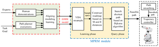
Figure 1.
The GMM/GMR-MPRM path planning framework.
The teacher will teach a specific task many times. After obtaining the data of the teaching path, the GMM/GMR module uses the GMM algorithm to obtain a compact data model according to the data of the teaching path, then the data model is fit into a smooth path with the mean and variance by GMR.
The function of the MPRM module is to generate a collision-free path based on the fit smooth path. Firstly, the smooth path is divided into a collision-free path and a collision path according to the position and shape of the obstacle. Then, the sampling space for the points on the collision path are generated using the variable density resampling method according to the covariance of the collision points and the relative position of the collision points and the obstacle, and the collision points in the sampling space are removed. Finally, a roadmap for the MPRM according to the EPD is constructed. After constructing the roadmap, the Dijkstra algorithm is used to search for a feasible path, then the Shortcut is used to prune the path and delete the redundant sampling points. A smooth path is generated by smoothing the pruned path using B-spline interpolation.
3. GMM/GMR Module
The GMM/GMR module is used to generate the sampling space based on the teaching data. Figure 2 gives the flowchart for generating the sampling space based on the GMM/GMR algorithm. First, according to the teaching path data, the GMM algorithm is used to obtain the Gaussian conditional distribution of the data of the teaching path, and then, the GMR algorithm is used to generate the task path and sampling space.
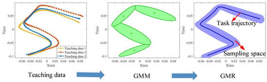
Figure 2.
The GMM/GMR-MPRM path planning framework.
Usually, the dataset of the teaching path consists of N teaching paths, so it can be represented by , where is one-time teaching path data. The teaching trajectory data are a sequence of random variables that obey the multivariate normal distribution. The GMM of the teaching data can be expressed as:
where stands for the coefficient of the Gaussian component and , , stands for the distribution density of the Gaussian component of dimensionality D, which can be defined as:
where , , and stand for the mean and variance of the Gaussian component, respectively, and can be expressed as:
The parameters of the GMM are solved using the EM algorithm. The solution steps are as follows: Firstly, the k-means clustering algorithm is used to obtain the initial estimated value of the EM algorithm to prevent the solution from falling into the local minima; secondly, the GMM infinitely approaches the optimal solution through the iteration of the E steps and M steps; finally, the parameters of the GMM that meet the requirements are obtained.
After using the GMM to obtain the distribution of the teaching trajectory, the GMR algorithm is used for regression to obtain a continuous path, and the path contains the mean and the covariance of each point on the path. Using time series as the index variables, the corresponding space vector is:
For a GMM , the GMM is transformed into a continuous model by varying t, according to the linear transformation properties of the Gaussian distribution, that is:
where,
For the totality component, the expected distribution is:
where is the prior probability of each component and can be expressed as:
For the component, the mean and covariance matrices of each time point can be computed as:
Then, a continuous trajectory can be generalized by calculating . The feasible space of the trajectory is used as the sampling space of the MPRM algorithm.
4. MPRM Module
The MPRM module consists of two parts: the construction part and the query part. In the construction part, by randomly sampling nodes in the free space and connecting them with each other, a roadmap can be constructed. In the query part, a path from the start location to the target location can be queried on the roadmap with the Dijkstra search algorithm. The conventional PRM methods uses a grid map in 2D space or a voxel map in 3D space to describe the roadmap. The roadmap covers the whole workspace, and once the environment changes, the roadmap has to be reconstructed. The MPRM module is used to generate robot motion from a given roadmap and the target location without a priori knowledge. However, in this paper, the GMM/GMR model already encoded the ideal robot motion. Therefore, it was able to combine these two methods and exploit their advantages so as to meet the online adaptive requirements.
4.1. Collision Detection and Path Segmentation
Before resampling, it is necessary to divide the path into a collision path and a noncollision path, that is to separate the collision path from the path and record the start and end points of the collision path.
In order to divide the path, it is necessary to calculate the Euclidean distance from the points on the path to the obstacle surface and then select the smallest Euclidean distance to compare with the threshold , where , stands for the radius of the obstacle, and stands for the radius of the manipulator of the robot. If , the point is considered to collide with the obstacle. The first collision point is recorded as the starting point of the collision path, then whether the next point is a collision point is determined, until the next point is a noncollision point, and the point is recorded as the end point of the collision path. Repeat the iteration until the last point on the path. The iterative process of the path segmentation algorithm is shown in Algorithm 1.
| Algorithm 1 Path segmentation algorithm. |
| Input: Task trajectory Output: The Startpoints and Endpoints of the collision path 1: Startpoints=[]; Endpoints=[]; StartFlag=False; EndFlag=False; 2: ; ; 3: while do 4: ; 5: if then 6: if Startflag==False then 7: Startflag=True; Startpoints(j)=i; ; 8: end if 9: else 10: if Startflag==True then 11: Startflag=False; Endpoints(j)=i; 12: end if 13: end if 14: end while |
4.2. Variable Density Resampling
Each point on the task path obtained by the GMM/GMR algorithm has a mean and a covariance. The mean value is represented by , and the covariance is represented by . This paper used the function in MATLAB to generate the sampling space. The function can generate a dataset that conforms to the multivariate Gaussian distribution. Therefore, resampling the point on the path based on the Gaussian distribution can be expressed as:
where is the resampled dataset of the point, is the sample quantity of resampling, and is the resampled dataset with a sample quantity of .
If the sample quantity of resampling for each Gaussian component on the task path is the same, then there will be a large number of resampling points near the obstacle when the Gaussian component close to the obstacle is resampled, which reduces the success rate of path planning. In addition, the covariance of the Gaussian component also has an impact on the quantity of resampling, that is the Gaussian component with a smaller covariance has higher importance, and the quantity of resampling for this component should be increased, while the Gaussian component with a larger covariance has lower importance, and the quantity of resampling for this component should be reduced.
Therefore, a variable density resampling method is proposed, that is the Gaussian component that is closer to the obstacle generates more sampling points, and the Gaussian component that is farther from the obstacle generates fewer sampling points. The Gaussian component with a small covariance generates more sampling points, and the Gaussian component with a high covariance generates fewer sampling points. This can not only increase the sampling speed and the success rate of path planning, but also improve the consistency of the planned path and the task path. The quantity of resampling can be defined as:
where is the shortest distance between the Gaussian component and the obstacle, is the threshold of the distance, is the covariance of the Gaussian component, and and are the reference quantity of resampling based on the covariance and distance, respectively. Since there is no collision detection during resampling, some sampling points will fall into the position of obstacles. If the roadmap is constructed directly in this sampling space, the number of collision detections and invalid queries will increase. Therefore, it is necessary to recalculate the minimum distance between the sampling point and the obstacle surface. If , the point is considered as the collision point and removed; otherwise, the point is retained.
4.3. Euclidean and Probability Distance
In the traditional PRM algorithm, the distance between two points is usually defined by the Euclidean distance between two points. The PRM algorithm adopted in this paper ensures that the shortest feasible path can be found, and it tries to ensure the similarity with the original trajectory. Therefore, this paper redefined the distance between two points as the weighted sum of the Euclidean distance and the probability distance, that is:
where represents the Euclidean distance between two points. is the coefficient with the value range of , used to balance the length of the planned path and the similarity with the task path, that is the larger is, the greater the similarity with the task path; the smaller is, the shorter the length of the planned path; represents the distance generated by the probability density.
The higher the probability density of the point is, the closer to the task path. Therefore, the probability distance is defined as the following form:
where , D is the dimension of the variable x, is the mean value, and is the covariance matrix.
Finally, according to the weighted distance , construct a locally weighted roadmap for each collision path, where is the edge and is the vertex.
4.4. Path Search Based on the Dijkstra Algorithm
The Dijkstra algorithm is one of the most famous algorithms for searching the shortest path. It uses the breadth-first search to solve the single-source shortest path problem of a weighted directed graph or an undirected graph. Given the roadmap , the starting vertex , and the target vertex , the shortest path from the starting point to the target point can be searched. Since the similarity with the task path is taken into account when constructing the roadmap, the algorithm follows the two principles of the shortest path and the highest similarity.
4.5. Path Pruning Based on the Shortcut Algorithm
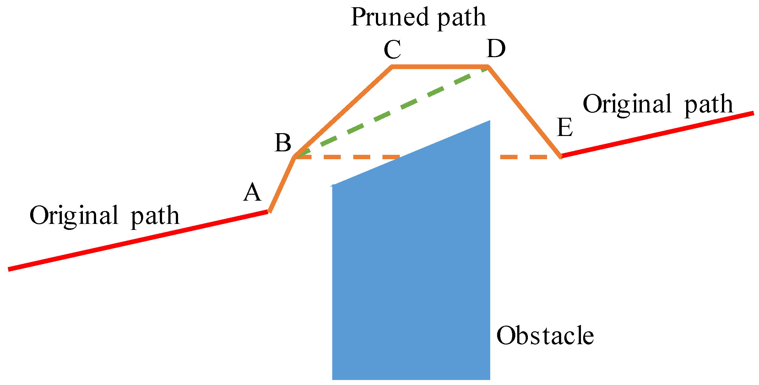
The Shortcut path pruning process is shown in Figure 3, assuming that the planned path is composed of Points A, B, C, D, and E. Although the trajectory can avoid the obstacle, it can be further simplified. For example, Point B can be directly connected to Point D, then Point C can be removed. However, when Point B and Point E are connected, they will collide with an obstacle, then Point D cannot be removed. The pruning algorithm is shown in Algorithm 2.

Figure 3.
Schematic diagram of path pruning.
| Algorithm 2 Shortcut path pruning algorithm. |
| Input: Path to be pruned path1 Output: Path after pruning path2 1: 2: ; 3:while do 4: for do 5: if then 6: ; 7: ; 8: break 9: end if 10: end for 11: end while |
4.6. B-Spline Trajectory Smoothing
After shortening the length of the path by using the Shortcut algorithm, B-spline interpolation is used to smooth the pruned path. At the same time, in order to ensure the continuous speed of the connection, the speed boundary condition is set. The B-spline curve is essentially a set of piecewise continuous polynomials, and complex curves can be described by low-order polynomials. The B-spline curve can be represented by:
where is the B-spline basis function, is the control vertex, and p is the order of the polynomial. The value of u is defined by the node vector:
Take , and use the Cox–de Boor recursion formula for the basis function of the B-spline; the recursion formula can be given by:
The shape of the B-spline curve is determined by the node vector and the control vertices. There are various parameterization methods to parameterize the node vector, such as uniform parameterization, chord length parameterization, and centripetal parameterization. Centripetal parameterization can obtain a smoother curve; therefore, this paper adopted this parameterization method:
where , and are the points to be interpolated.
For the cubic B-spline curve, when performing the interpolation calculation, there is:
This formula can be expressed in the form of the matrix equation:-4.6cm0cm
For the cubic B-spline curve, the first and last nodes in the node vector are quadruple nodes, and this causes the first (end) vertex to be the same as the first (end) data point. After removing the first and last two equations of the above formula, the matrix equation can be expressed as:
Add two boundary conditions and simplify; the matrix equation can be expressed as:
where,
The velocity boundary conditions are:
Therefore, given the boundary velocities and , an interpolated B-spline curve with a continuous velocity can be obtained.
5. Simulation and Experimental Analysis
5.1. Simulation and Analysis
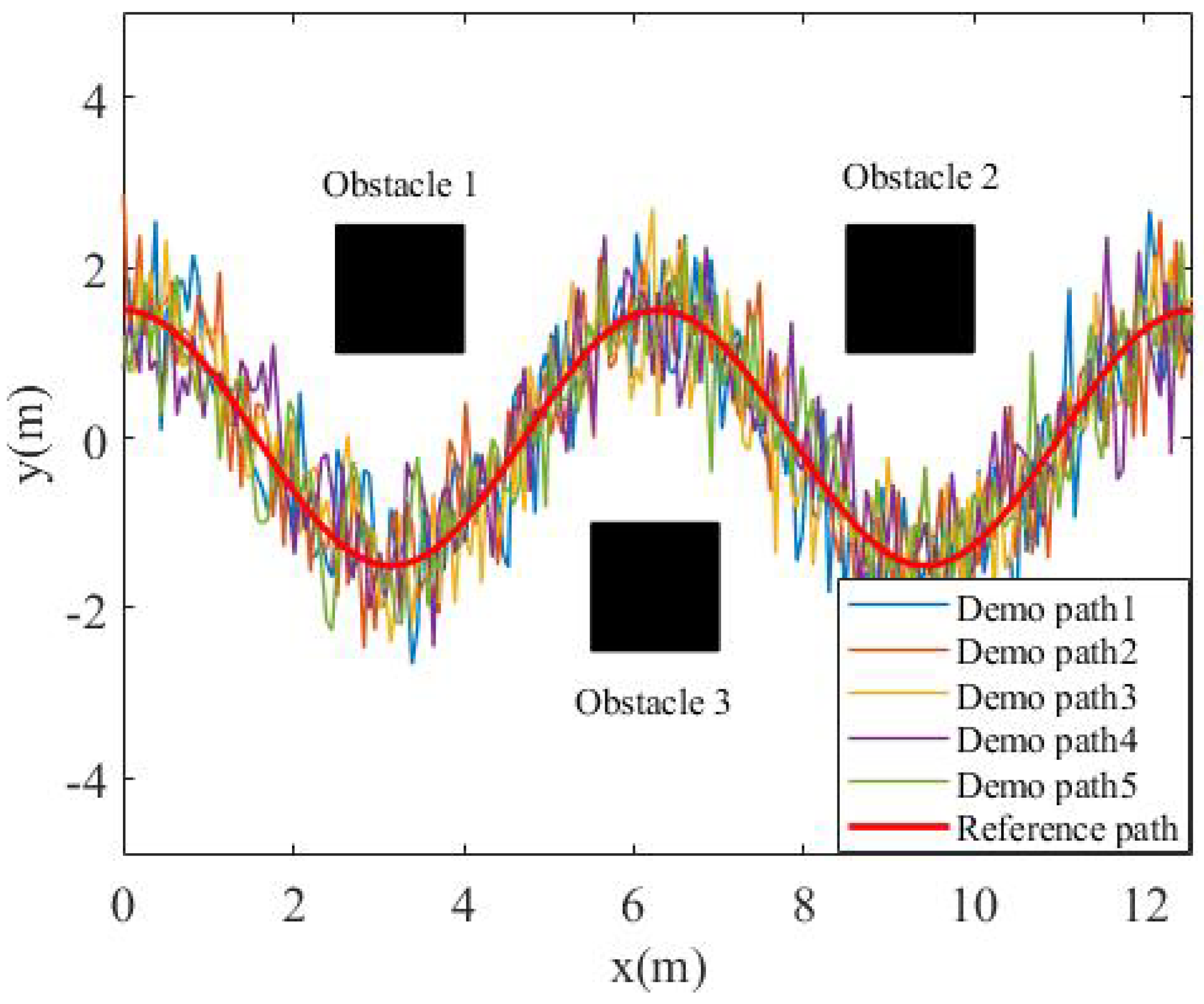
In order to verify the effectiveness of the algorithm, this paper constructed a simulation scenario in MATLAB. The purpose of the experiment was to plan a motion path close to the task trajectory, and there were three obstacles around the task trajectory. The task trajectory was a cosine curve of two periods, that is: .
In order to simulate the uncertainty in the demonstration data, the task trajectory was first enlarged by 0.9, 0.96, 1, 1.03, and 1.1 times, and then, 6dB of Gaussian noise was added to obtain the teaching data, as shown in Figure 4. Finally, the GMM algorithm was used to model the loose teaching data, as shown in Figure 5. The number of Gaussian components in the GMM was set as , and it can be seen that the data expressed by the GMM were relatively compact.

Figure 4.
Demonstration environment.
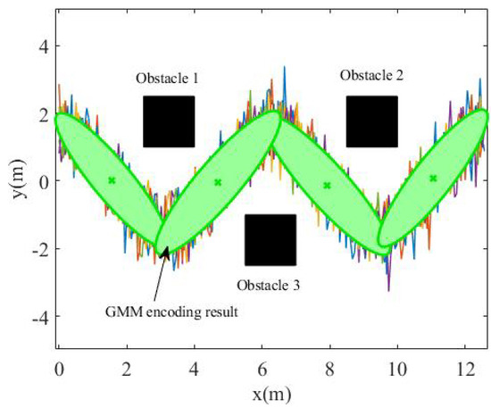
Figure 5.
GMM encoding result.
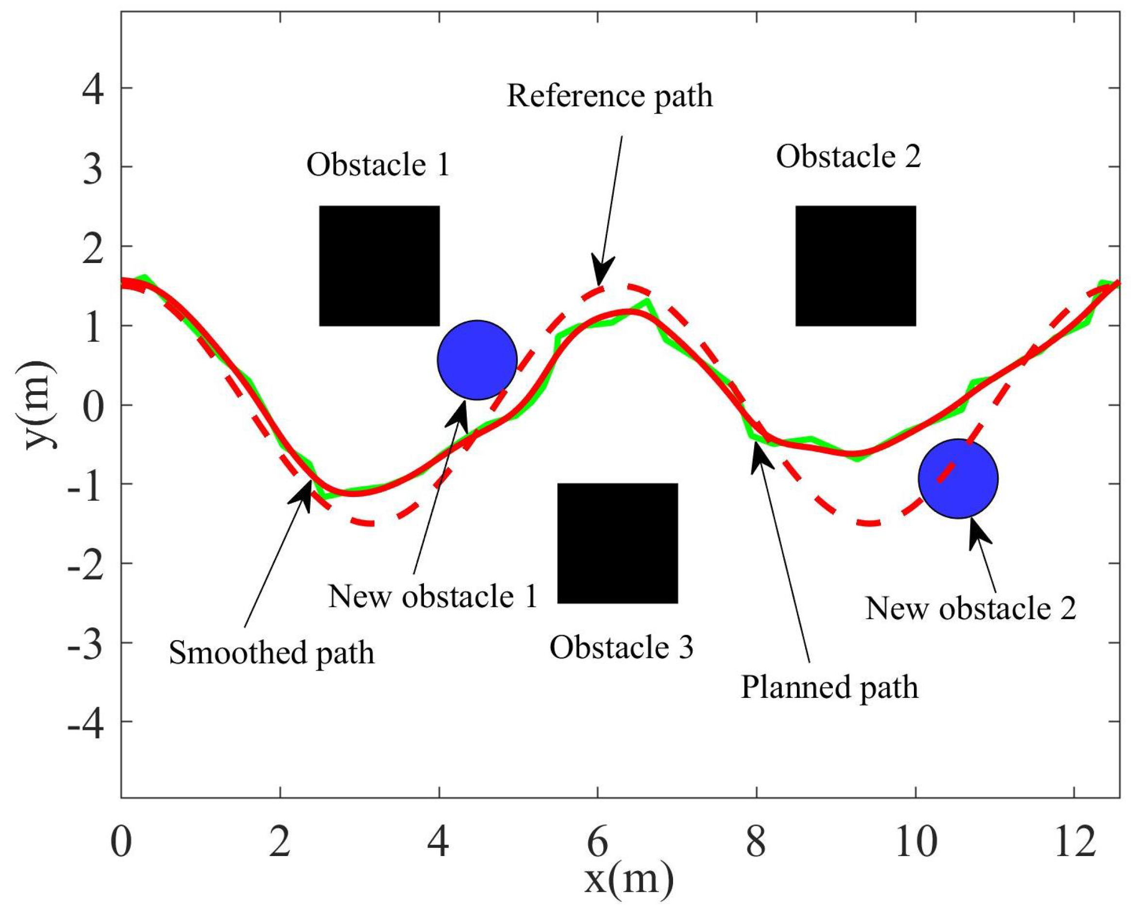
After using the GMM algorithm to transform the demonstration data into a compact probability model, the GMR algorithm was used to fit the model into a smooth path with variance as the resample space for path planning. However, there will be a certain difference between the recurrent scene and the teaching scene. Two obstacles were added to the recurrent scene to indicate the difference from the teaching scene. The recurrent scene can seen in Figure 6; it can be seen that the path planned using GMR will collide with the obstacle.
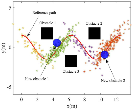
Figure 6.
The recurrent scene with two new obstacle.
In order to plan a path that is not only able to avoid new obstacles, but is also similar to the original trajectory, the original trajectory was divided into the collision-free path and the collision path. According to the distance between the obstacles and the points in the sampling space, variable density resampling was carried out to generate uneven sampling points and remove the points that collide with obstacles. A roadmap was constructed according to the EPD, then Dijkstra algorithm was used to search the feasible path. Finally, the planned path was pruned and smoothed to generate a smooth path. In the simulation, the quantity of resampling based on covariance was set as , the quantity of resampling based on distance was set as , and the adjustment coefficient of the Euclidean and probability distances was , while the order of the B-spline was set as . The path planned by the GMM/GMR-MPRM is shown in Figure 7, and it can be seen from the figure that the GMM/GMR-MPRM can still plan a feasible path when the recurrent scene is not the same as the teaching scene.
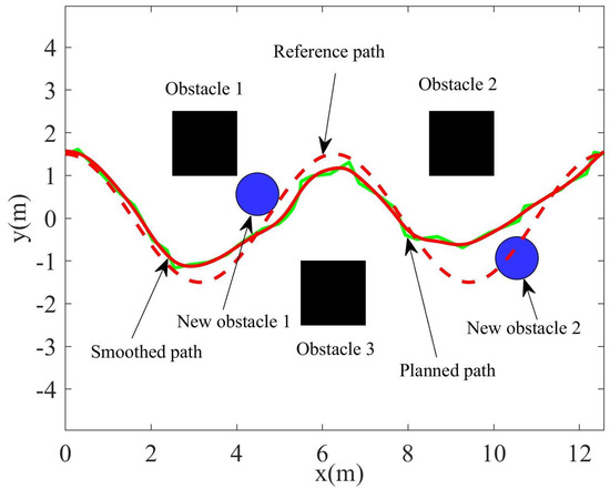
Figure 7.
Path planned by the GMM/GMR-MPRM.
5.2. Experiment and Analysis
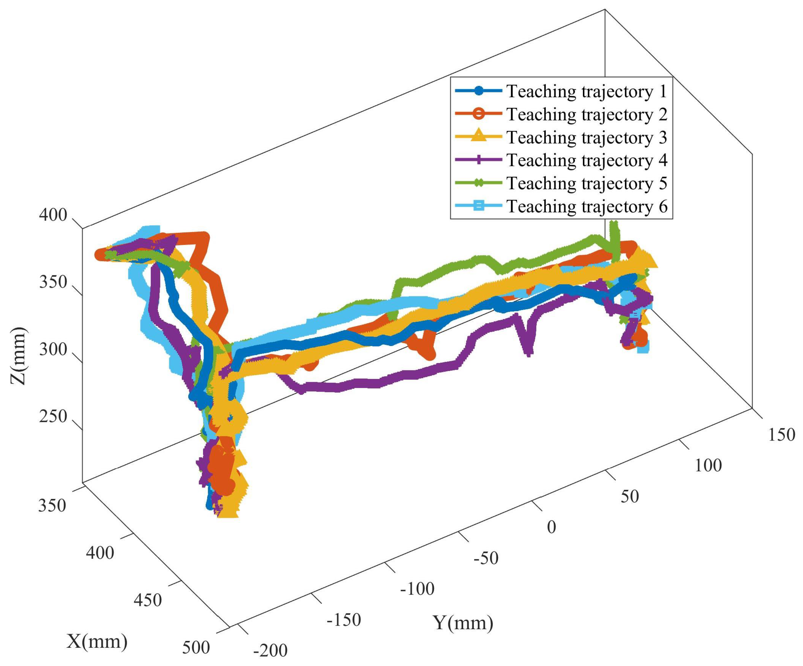
In order to verify the effectiveness of the GMM/GMR-MPRM algorithm, a path planning experiment platform for the pick-and-place task of a manipulator was built. The manipulator used in this experimental platform was ABB IRB1200, with a maximum load of 7 kg and a maximum working radius of 700 mm. The manipulator was installed on the workbench, and a pneumatic gripper was installed at the end of the manipulator to complete tasks such as picking and placing and assembly. A Kinect V2 was also installed on the workbench to detect the position and size of the obstacle. The experimental platform is shown in Figure 8. In this experimental scene, the manipulator needed to pick up the axle from the container and place it in another container. In the process of the demonstration, the teacher performed teaching six times, and six different teaching trajectories were obtained, as shown in Figure 9. When the task recurred, a white spherical obstacle with a diameter of 50 mm was placed on the task path. The position and size of the obstacle were obtained by the Kinect V2, and the position of the obstacle was .
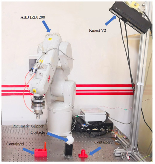
Figure 8.
The experimental platform.

Figure 9.
Teaching trajectory of the experimental task.
Because there was an obstacle in the experimental scene, if the pick and place task were executed directly according to the path planned by the GMM/GMR, it would cause the manipulator to collide with the obstacle. However, the obstacle did not affect all the feasible space of the teaching path, but only part of the feasible space. Therefore, the GMM/GMR-MPRM algorithm can be used for trajectory planning. The number of Gaussian components in the GMM was set as . The quantity of resampling based on covariance was set as . The quantity of resampling based on the distance was set as . The adjustment coefficient of the Euclidean and probability distances was . The order of the B-spline was set as . The control loop rate of IRB1200 was 10 Hz.
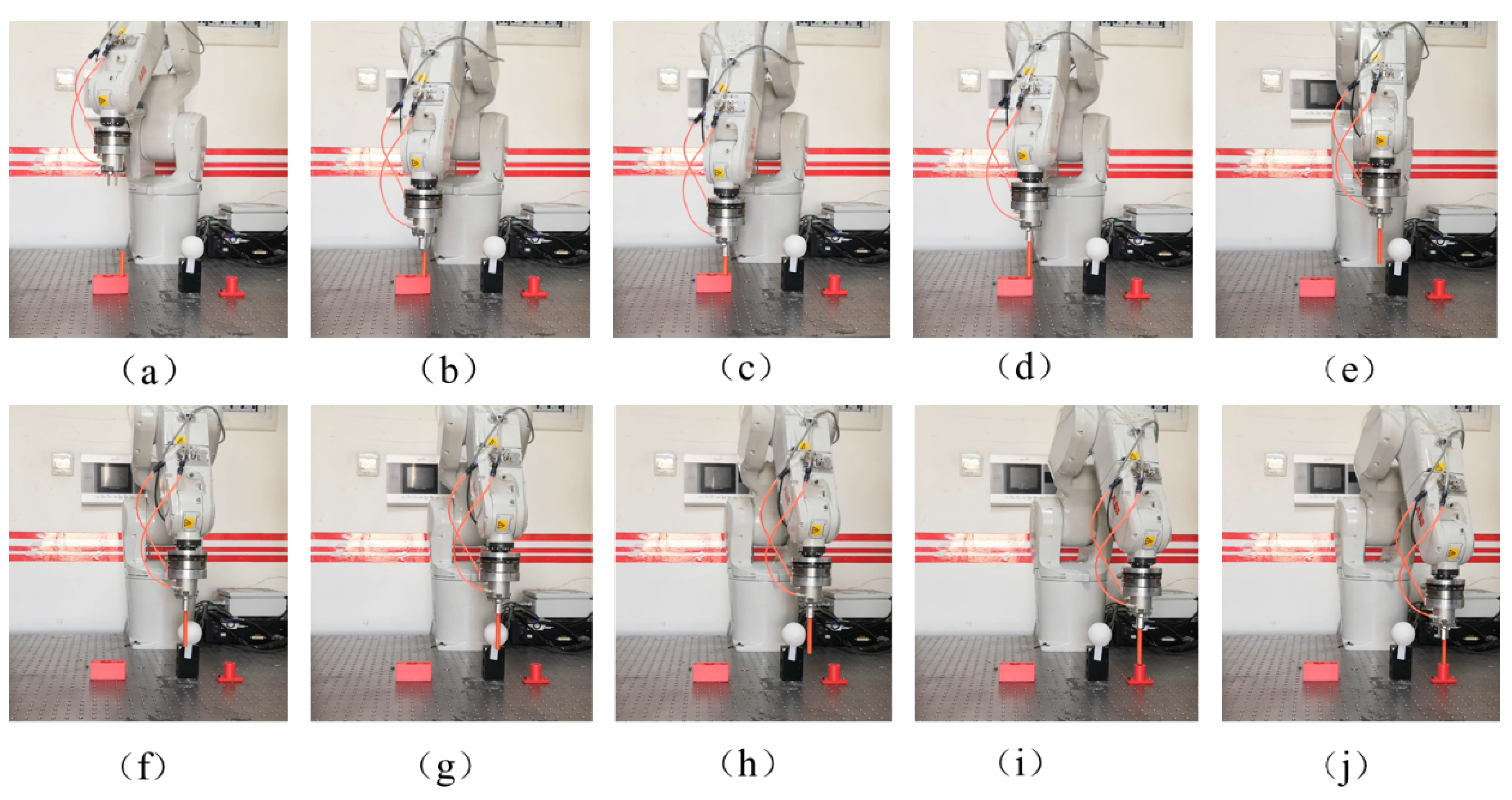
Figure 10 is the path planning process of the manipulator using the GMM/GMR-MPRM algorithm: (a,b) the manipulator first moves to the initial position and then moves to the top of the container; (c) the manipulator descends to the grasping position and grabs the shaft; (d,e) after the grasping is completed, the manipulator is raised to a certain height and then moved to the vicinity of the obstacle; (e–h) there is a feasible space in front of the obstacle, and the GMM/GMR-MPRM algorithm plans a feasible path in this space; the manipulator bypasses the front side of the obstacle; (h–j) after the manipulator completes the obstacle avoidance, the manipulator continues to move to the top of the container along the GMR path, moves downwards, and opens the claw to release the shaft, then the shaft is placed into the container.
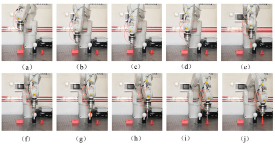
Figure 10.
Path planning process for the manipulator with the GMM/GMR-MPRM algorithm. (a–j) are the different stages of the manipulator in completing the task.
The experimental results showed that the GMM/GMR-MPRM algorithm provided the manipulator better adaptability when the task recurred, that is when a new obstacle appeared in the recurring scene, the path planning could be completed without teaching again.
6. Conclusions
In this paper, we proposed an adaptive path planning algorithm aiming at the problem of a task recurring in the process of LfD. The algorithm was based on the GMM of the teaching path and used the GMR algorithm to generate the task path and sampling space. Then, the steps of collision detection, path segmentation, variable density resampling, EPD-based roadmap construction, Dijkstra path search, Shortcut path pruning, and the smooth path of the B-spline were followed. Finally, a smooth and feasible task path was generated.
The sampling space obtained by the algorithm not only met the physical constraints and task constraints, but also reduced the size of the sampling space and improved the speed of motion planning. Variable density resampling can improve the efficiency and success rate of motion planning. The route map constructed by the Euclidean distance and the probability distance can ensure that the planned path is shorter and closer to the task trajectory.
Author Contributions
Literature search, software, data curation, and writing—original draft, Q.C.; data interpretation, H.L. and Y.Z.; methodology, Q.C. and W.Z.; writing—review and editing, H.L., Y.Z. and L.H. All authors have and agreed to the published version of the manuscript.
Funding
This work was supported by the National Natural Science Foundation of China under Grant Number 62073063 and the Fundamental Research Funds for the Central Universities under Grant Numbers N18240007-2, N2104008, and N2003003.
Institutional Review Board Statement
Not applicable.
Informed Consent Statement
Not applicable.
Data Availability Statement
The data are contained within the article.
Acknowledgments
We thank Xingchen Li for his comments, which substantially improved the quality of this paper.
Conflicts of Interest
The authors declare no conflict of interest.
References
- Zhou, Z.; Hu, J.; Wang, Y.; Xiong, R. Research progress of robot programming by demonstration. Autom. Panor. 2020, 37, 48–56. [Google Scholar]
- Russo, M.; Cafolla, D.; Ceccarelli, M. Design and experiments of a novel humanoid robot with parallel architectures. Robotics 2018, 7, 79. [Google Scholar] [CrossRef] [Green Version]
- Ceccarelli, M.; Cafolla, D.; Carbone, G.; Russo, M.; Cigola, M.; Senatore, L.J.; Gallozzi, A.; Maccio, R.D.; Ferrante, F.; Bolici, F.; et al. HeritageBot service robot assisting in cultural heritage. In Proceedings of the 2017 First IEEE International Conference on Robotic Computing, Taichung, Taiwan, 10–12 April 2017; pp. 440–445. [Google Scholar]
- Kavraki, L.E.; Svestka, P.; Latombe, J.; Overmars, M.H. Probabilistic roadmaps for path planning in high-dimensional configuration spaces. Int. Trans. Robot. Autom. 1996, 12, 566–580. [Google Scholar] [CrossRef] [Green Version]
- LaValle, S.M.; Kuffner, J.J. Rapidly-exploring random trees: Progress and prospects. In Algorithmic and Computational Robotics; Donald, B., Lynch, K., Rus, D., Eds.; A K Peters/CRC Press: New York, NY, USA, 2001; pp. 293–308. [Google Scholar]
- Wei, K.; Ren, B. A Method on Dynamic Path Planning for Robotic Manipulator Autonomous Obstacle Avoidance Based on an Improved RRT Algorithm. Sensors 2018, 18, 571. [Google Scholar] [CrossRef] [PubMed] [Green Version]
- Bohlin, R.; Kavraki, L.E. Path planning using lazy PRM. In Proceedings of the 2000 IEEE International Conference on Robotics and Automation, San Francisco, CA, USA, 24–28 April 2000; pp. 521–528. [Google Scholar]
- Hsu, D.; Latombe, J.C.; Motwani, R. Path Planning in Expansive Configuration Spaces. In Proceedings of the 1997 IEEE International Conference on Robotics and Automation, Albuquerque, NM, USA, 25–25 April 1997; pp. 2719–2726. [Google Scholar]
- Sánchez-Ante, G. Path planning using a single-query bi-directional lazy collision checking planner. In Proceedings of the Mexican International Conference on Artificial Intelligence, Yucatan, Mexico, 22–26 April 2002; pp. 41–50. [Google Scholar]
- Kuffner, J.J.; LaValle, S.M. RRT-Connect: An Efficient Approach to Single-Query Path Planning. In Proceedings of the 2000 IEEE International Conference on Robotics and Automation, San Francisco, CA, USA, 24–28 April 2000; pp. 995–1001. [Google Scholar]
- Wang, X.; Luo, X.; Han, B.; Chen, Y.; Liang, G.; Zheng, K. Collision-free path planning method for robots based on an improved rapidly-exploring random tree algorithm. Appl. Sci. 2020, 10, 1381. [Google Scholar] [CrossRef] [Green Version]
- Şucan, I.A.; Kavraki, L.E. Kinodynamic Motion Planning by Interior-Exterior Cell Exploration. In Algorithmic Foundation of Robotics VIII; Chirikjian, G.S., Choset, H., Morales, M., Murphey, T., Eds.; Springer: Berlin/Heidelberg, Germany, 2009; pp. 449–464. [Google Scholar]
- Elbanhawi, M.; Simic, M. Sampling-Based Robot Motion Planning: A Review. IEEE Access 2014, 2, 56–77. [Google Scholar] [CrossRef]
- Jaillet, L.; Cortés, J.; Siméon, T. Sampling-Based Path Planning on Configuration-Space Costmaps. IEEE Trans. Robot. 2010, 26, 635–646. [Google Scholar] [CrossRef] [Green Version]
- Karaman, S.; Frazzoli, E. Sampling-based Algorithms for Optimal Motion Planning. Int. J. Robot. Res. 2011, 30, 846–878. [Google Scholar] [CrossRef]
- Gammell, J.D.; Srinivasa, S.S.; Barfoot, T.D. Batch informed trees (BIT*): Sampling-based optimal planning via the heuristically guided search of implicit random geometric graphs. In Proceedings of the 2015 IEEE International Conference on Robotics and Automation, Seattle, WA, USA, 26–30 May 2015; pp. 3067–3074. [Google Scholar]
- Chen, Y.; Roveda, L.; Braun, D.J. Efficiently Computable Constrained Optimal Feedback Controllers. IEEE Robot. Autom. Lett. 2018, 4, 121–128. [Google Scholar] [CrossRef]
- Shin, S.Y.; Lee, J.W.; Kim, C.H. Humanoid’s dual arm object manipulation based on virtual dynamics model. In Proceedings of the 2012 IEEE International Conference on Robotics and Automation, Saint Paul, MN, USA, 14–18 May 2012; pp. 2599–2604. [Google Scholar]
- Shahid, A.A.; Roveda, L.; Piga, D.; Braghin, F. Learning continuous control actions for robotic grasping with reinforcement learning. In Proceedings of the 2020 IEEE International Conference on Systems, Man, and Cybernetics (SMC), Toronto, ON, Canada, 11–14 October 2020; pp. 4066–4072. [Google Scholar]
- Schaal, S. Dynamic Movement Primitives—A Framework for Motor Control in Humans and Humanoid Robotics. In Adaptive Motion of Animals and Machines; Kimura, M., Tsuchiya, K., Ishiguro, A., Witte, H., Eds.; Springer: Tokyo, Japan, 2006; pp. 261–280. [Google Scholar]
- Roveda, L.; Magni, M.; Cantoni, M.; Piga, D.; Bucca, G. Human-Robot Collaboration in Sensorless Assembly Task Learning Enhanced by Uncertainties Adaptation via Bayesian Optimization. Robot. Auton. Syst. 2020, 136, 103711. [Google Scholar] [CrossRef]
- Rai, T.; Meier, F.; Ijspeert, A.; Schaal, S. Learning coupling terms for obstacle avoidance. In Proceedings of the 2014 IEEE-RAS International Conference on Humanoid Robots, Madrid, Spain, 18–20 November 2014; pp. 512–518. [Google Scholar]
- Amir, M.; Chris, P.; Luca, B. An incremental approach to learning generalizable robot tasks from human demonstration. In Proceedings of the 2015 IEEE International Conference on Robotics and Automation, Seattle, CA, USA, 26–30 May 2015; pp. 5616–5621. [Google Scholar]
- Jiang, X.; Kallmann, M. Learning humanoid reaching tasks in dynamic environments. In Proceedings of the 2007 IEEE/RSJ International Conference on Intelligent Robots and Systems, San Diego, CA, USA, 29 October–2 November 2007; pp. 1148–1153. [Google Scholar]
- Rosell, J.; Suárez, R.; Pérez, A. Path planning for grasping operations using an adaptive PCA-based sampling method. Auton. Robot. 2013, 35, 27–36. [Google Scholar] [CrossRef] [Green Version]
- García, N.; Rosell, J.; Suárez, R. Motion planning using first-order synergies. In Proceedings of the 2015 IEEE/RSJ International Conference on Intelligent Robots and Systems, Hamburg, Germany, 28 September–2 October 2015; pp. 2058–2063. [Google Scholar]
- Phillips, M.; Cohen, B.; Chitta, S.; Likhachev, M. E-Graphs: Bootstrapping Planning with Experience Graphs. In Proceedings of the Robotics: Science and Systems Conference, Sydney, Australia, 9–13 July 2012. [Google Scholar]
- Phillips, M.; Hwang, V.; Chitta, S.; Likhachev, M. Learning to plan for constrained manipulation from demonstrations. Auton. Robot. 2016, 40, 109–124. [Google Scholar] [CrossRef]


Publisher’s Note: MDPI stays neutral with regard to jurisdictional claims in published maps and institutional affiliations. |
© 2021 by the authors. Licensee MDPI, Basel, Switzerland. This article is an open access article distributed under the terms and conditions of the Creative Commons Attribution (CC BY) license (https://creativecommons.org/licenses/by/4.0/).