Classification of Electricity Consumption Behavior Based on Improved K-Means and LSTM

Featured Application

The results of this work will be used to develop a classification framework that will be applied in the analysis of a large number of scattered users’ electricity consumption behavior. This work sets labels for existing electricity consumption behaviors to carry out the classification of unknown types of electricity consumption behavior.

Abstract

Power big data-based artificial intelligence or data mining methods, which can be used to analyze electricity consumption behavior, have been widely applied to provide targeted marketing services for electricity consumers. However, the traditional clustering algorithm has difficulty in judging new electricity consumption patterns. Deep neural networks usually need large amounts of labeled data. However, there are few comparable electricity consumption features or basic data, and the labeled data cannot meet the actual needs. Therefore, an intelligent classification framework for electricity consumption behavior based on an improved k-means and long short-term memory (LSTM) is proposed, which not only extracts features effectively, but also establishes a mapping relationship between unlabeled electricity consumption behavior characteristics and user types. The features can be labeled to train the deep neural network to judge the electricity consumption behavior of new users. Firstly, nine typical characteristics were selected from aspects including electricity price sensitivity and load fluctuation rate. Secondly, the k value and initial clustering centers of the k-means algorithm were optimized. Thirdly, the users were labelled based on the clustering results, together with the features, and a dataset was formed, which was input into LSTM to train the classification model. Finally, the analysis of users in Shenyang, China, showed the results based on the proposed method were consistent with the actual situation. Moreover, compared to other methods, the efficiency and accuracy were higher.

1. Introduction

Based on power big data, artificial intelligence or data mining techniques can be reasonably applied to the analysis of user electricity consumption behavior and habits, which can help power grids to understand the characteristics of users’ electricity consumption and provide more targeted electricity services and marketing strategies [1,2,3]. However, with regard to dispersed and distinct power big data, how to choose appropriate data analysis methods, how to select effective features, and how to make full use of historical data to achieve detailed classification of electricity consumption behavior are all unsolved problems.

At present, the methods commonly used in electricity behavior analysis are cluster analysis and deep neural networks [4]. A clustering method based on self-organizing maps and k-means was proposed in [5], where the self-organizing map was used to initially select cluster centers, which significantly improved the accuracy of clustering and reduced the convergence time of the algorithm. In [6], principal component analysis was introduced to extract features from the original data, and then these features were used as the input of fuzzy clustering, which effectively improved the efficiency of the clustering. In [7], affinity propagation clustering was used in the analysis of electricity consumption. The discrete characteristics and time domain features obtained by symbolic aggregate approximation were extracted. The load curve was reduced in dimensionality and has been fully described. In [8], based on a correlation analysis, cluster forecasting was carried out for each type of load, which not only considered the electricity consumption characteristics of each type of load but also clustered the loads with similar characteristics, reducing the error of load forecasting. In [9], a method based on a simulated annealing algorithm for the optimization of initial cluster centers was proposed, which improved the performance of the k-means algorithm. A pattern classification of an electricity consumption curve based on auto-encoding neural network and fuzzy c-means clustering was proposed in [10], and the optimized electricity price model was established for different electricity consumption patterns, which could guide users to adjust electricity consumption behavior and electricity purchase strategies. Deep neural networks are generally used in load forecasting and classification. A load forecasting method based on a deep belief network (DBN) was proposed in [11]. The potential environmental factors with the strongest correlation with the electricity consumption behavior were selected as inputs to improve the forecasting accuracy. A user classification method based on hybrid long short-term memory (H-LSTM) neural network was proposed in [12]. The H-LSTM neural network analyzed the temporal correlation of feature sequences, and then obtained the classification results.

The above methods focused on the improvement of clustering algorithms or the optimization of features, and the cluster analyses were only performed on the existing data. If new electricity consumption data appears, re-clustering will take a lot of time. Additionally, deep neural networks are often used for load forecasting and require a large amount of label data.

The main contributions of this paper are summarized as follows:

(1)

A framework for intelligent classification of electricity consumption behavior based on improved k-means and LSTM is proposed, which can judge users’ electricity consumption behavior accurately.

(2)

An improved k-means clustering method is introduced to set labels for scattered and irregular original data, and the initial k value and initial clustering centers of the k-means algorithm are optimized intelligently.

The remainder of this paper is organized as follows: Section 2 proposes the classification framework for electricity consumption behavior based on improved k-means and LSTM. Section 3 delivers the defined characteristics and the improved k-means clustering algorithm, as well as the basic network framework of LSTM. Section 4 analyzes the electricity consumption behavior of SY city in LN Province, China, based on the proposed method. Section 5 concludes the paper.

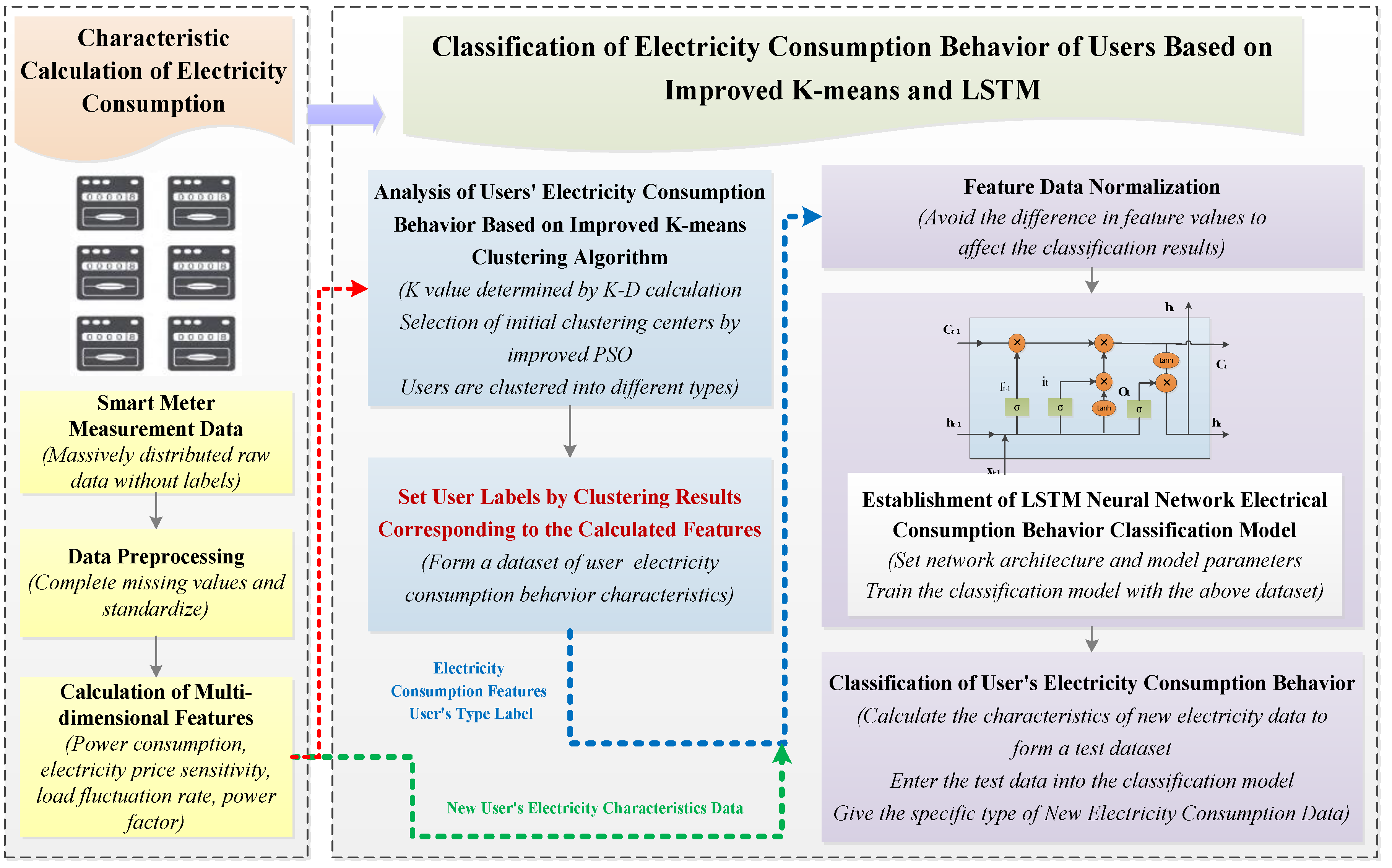
2. The Framework of Electricity Consumption Behavior Classification Based on Improved K-Means and LSTM

Electricity consumption behavior classification based on improved k-means and LSTM mainly includes selecting electricity characteristics and electricity consumption behavior classification. In order to form an effective feature set to train the classification model, cluster analysis was performed. Based on the clustering results, the labels for each user were set corresponding to the extracted features. Then, the intelligent classification model was achieved. The framework is shown in Figure 1.

The specific steps corresponding to the framework are as follows:

• Data acquisition: The electricity consumption data of a certain period were acquired by smart meters. Then, the incomplete data in the original data were replaced with values (average or median) close to the center of the sample attribute. In order to avoid the impact of data differentiation, the above preprocessed data were normalized.
• Feature selection: Multi-dimensional features were calculated based on the preprocessed data, which included electricity consumption, electricity price sensitivity, load fluctuation rate, and power factor.
• Cluster analysis: Referring to the calculated features, we performed a preliminary clustering of users. In order to improve the performance of clustering, the traditional k-means algorithm was improved.
• Training classification model: We initialized the LSTM network structure and selected model parameters. Based on the results of clustering, the users’ labels were set. Together with the calculated features, the electricity consumption behavior dataset was formed, which was used as an input to train the LSTM classification model, and then the trained model parameters were saved.
• Evaluation of classification results: We obtained new electricity consumption data from smart meters and calculated features through the same steps as above. Then, we input the new features into the trained LSTM, and output the classification results to judge the users’ electricity consumption behavior. Finally, the performance of the model was evaluated, and the classification results of other models were compared.

3. Analysis Method of Users’ Electricity Consumption Behavior

3.1. Multi-Dimensional Feature Extraction

There are two common clustering methods for electricity consumption behaviors: direct clustering and indirect clustering. Direct clustering includes k-means, hierarchical clustering, density-based spatial clustering with noise, and self-organizing maps. Indirect clustering requires the performance of feature extraction on the electricity data before clustering. Good feature extraction can greatly improve the effect of clustering [2].

The user’s electricity consumption behaviors are related to multiple factors, such as load, price, time, and environment. There are many characteristics used to describe the behavior, including the daily load rate, valley electricity coefficient, peak time power consumption rate, daily minimum, and maximum load [13,14]. According to different electricity consumption characteristics, different electricity consumption behaviors can be derived.

However, there are few horizontally comparable features and basic data that can be obtained. Some defined features are difficult to meet the actual needs [15,16]. In this paper, a set of electricity consumption characteristics based on power big data (mainly including active load, reactive load, electricity consumption, and electricity price) are proposed, which take into account four aspects: electricity consumption, electricity price sensitivity, load fluctuation rate, and power factor.

• Electricity consumption characteristics.

The total electricity consumption reflects the user’s electricity consumption capacity, which is closely related to the type of the user. It is shown as:

$$A={\displaystyle \sum _{i=1}^{24}P(i)\Delta T}$$

(1)

where $A$ is the total electricity consumption in one day; $P(i)$ is the active power per hour; $\Delta T$ is the time interval, which is 1 h. The total electricity consumption is related to the composition and load adjustment measures of users.

• Sensitivity of electricity price.

Electricity price sensitivity includes sensitivity of electricity price changes and sensitivity of total electricity price.

(a) Sensitivity of electricity price changes:

$$SS={\displaystyle \sum _{i=1}^{24}F(i)}$$

(2)

$$F(i)=\{\begin{array}{l}0,\hspace{1em}\hspace{1em}T(i+1)-T(i)=0\\ \frac{P(i+1)-P(i)}{T(i+1)-T(i)},\hspace{1em}\hspace{1em}T(i+1)-T(i)\ne 0\end{array}$$

(3)

where $SS$ represents the sensitivity of electricity price change; $F(i)$ represents the electricity price change at each hour. $P(i)$ represents the active power at time $i$; $P(i+1)$ represents the active power at time $i+1$; $T(i)$ represents the electricity price at time $i$; $T(i+1)$ represents the electricity price at time $i+1$.

(b) Sensitivity of total electricity price:

$$S{T}_1=\frac{W_1}{T_1}$$

(4)

$$S{T}_2=\frac{W_2}{T_2}$$

(5)

$$S{T}_3=\frac{W_3}{T_3}$$

(6)

where $S{T}_1$, $S{T}_2$, and $S{T}_3$ are the sensitivity of total electricity price in the valley, flat, and peak period, respectively; $W_1$, $W_2$, and $W_3$ are the electricity consumption in the valley, flat, and peak period, respectively. $T_1=0.4$ is the electricity price in the valley period; $T_2=0.8$ is the electricity price in the flat period; and $T_3=1.2$ is the electricity price in the peak period.

The above two parameters can reflect the users’ electricity demand changes with electricity prices. The higher the electricity price sensitivity, the greater the load. Conversely, the lower the electricity price sensitivity, the smaller the load.

• Load fluctuation rate.

Load fluctuation rate includes the peak–valley difference, the mean square deviation, and the ramps.

(a) Peak–valley difference:

$$DPN=\max (P(i))-\min (P(i))$$

(7)

where $DPN$ is the peak–valley difference, which is equal to the difference between $\max (P(i))$ (maximum active power) and $\min (P(i))$ (minimum active power) at time $i$. The index is closely related to the fluctuation of electricity consumption and season.

The greater the peak–valley difference, the greater the peak-shaving pressure of the grid, and the greater the peak-shaving capacity required to maintain the safe operation of the grid.

(b) Mean square deviation:

$$MSE=\sqrt{\frac{1}{24}{\displaystyle \sum _{i=1}^{24}{(P(i)-\overline{P})}^2}}$$

(8)

where $MSE$ represents the mean square deviation; $P(i)$ is the active power at $i$; $\overline{P}$ is the average active power of a day.

The mean square deviation can reflect the dispersion degree of active power of the user at 24 h. The larger the mean square deviation, the greater the user’s load fluctuation rate. The smaller the mean square deviation, the smaller the user’s load fluctuation rate, and the more stable the load.

(c) Ramps:

$$R={\displaystyle \sum _{i=1}^{23}{(P(i+1)-P(i))}^2}$$

(9)

where $R$ represents ramps; $P(i)$ represents the active power at $i$; $P(i+1)$ represents the active power at $i+1$. In peak or low periods of load, ramping events pose a great threat to the safe operation of a power system.

• Power factor.

The power factor reflects the utilization rate of electrical equipment from a technological perspective and the economic benefits of a grid from a management perspective. The minimum power factor is selected as the characteristic:

$$MINPF=\min (P(i)/Q(i))$$

(10)

where $MINPF$ is the minimum power factor; $P(i)$ is the active power at $i$; $Q(i)$ is the reactive power at $i$. The higher the power factor, the higher the equipment utilization rate, and the better the economic efficiency of the grid.

Based on the above index, each user’s electricity consumption behavior is expressed as a 1 × 9 vector $X=[A,SS,S{T}_1,S{T}_2,S{T}_3,DPN,MSE,R,MINPF]$. In order to avoid the influence of larger or smaller values, $X$ is normalized. Using $X$ as a reference, the cluster analysis is performed on the user’s electricity consumption behavior.

3.2. Optimization of K Value

Cluster analysis of users’ electricity data can divide a large number of scattered users into k typical electricity consumption patterns, which is helpful for further refining electricity consumption characteristics. A k-means clustering algorithm is simple and efficient, and with fast convergence and strong scalability, which is often used in the study of electricity consumption behavior [17,18,19].

A k-means algorithm needs to specify the number of clusters k in advance. However, the k is usually given by experience, without considering the actual characteristics of the sample, which is subjective. Therefore, a k value selection strategy based on the K-D calculation was proposed.

Firstly, select a point as the first clustering center in feature dataset. Secondly, calculate the distance $D(x)$ between each point and the selected cluster center. The smaller the $D(x)$, the greater the probability that that point is selected as the new cluster center. Then, repeat the calculation until k cluster centers are selected. Finally, use these k values as the initial cluster centers, and the k value can be obtained from the K-D curve.

$$D=\frac{D_1}{D_2}$$

(11)

where $D$ is the distance between each point and the nearest cluster center; $D_1$ is the average distance within the cluster; and $D_2$ is the average distance between clusters. The smaller the $D$, the smaller the intra-class distance, or the larger the inter-class distance.

The common distance calculation methods of a k-means algorithm are cosine similarity and Euclidean distance. We adopted the latter and took the square root of the minimum Euclidean distance as the objective function.

3.3. Optimization of Initial Clustering Centers

The initial clustering centers of the traditional k-means algorithm is randomly given, which may cause the algorithm to fall into a local optimum, and the final result will be unstable. Therefore, an improved particle swarm optimization (PSO) algorithm for initial cluster centers optimization is proposed. The PSO algorithm does not have many adjustment parameters, which is simple and can be used for a wide range of applications. The algorithm has been introduced many times in the literature [20,21].

The improved PSO algorithm proposed in this paper mainly selects the inertial weight factor and the learning factor by adjusting the parameters, which avoids the algorithm from falling into the local optimum and being difficult to converge when searching the optimal solution.

Supposing the initial clustering centers composed of $N$ particles are searched in the $D$ dimensional space, the position of the $\mathit{i-}th$ particle is $x_{id}=(x_{i1},x_{i2},\dots x_{id})$, and the flight speed is $v_{id}=(v_{i1},v_{i2},\dots ,v_{iD})$, where, $i=1,\dots ,N$. After determining the optimal solution, the particle swarm updates the position and velocity according to (12) and (13) [22].

$$v_{id}^{k+1}=w{v}_{id}^k+c_1{r}_1(p_i^k-x_{id}^k)+c_2{r}_2(p_g^k-x_{id}^k)$$

(12)

$$x_{id}^{k+1}=x_{id}^k+v_{id}^{k+1}$$

(13)

where $k$ is the number of iterations; $w$ is the inertia weight factor; $c_1$ and $c_2$ are the learning factor, and their values are reported in [1,2]. Their appropriate value can accelerate the convergence rate and avoid falling into the local optimum. $r_1$ and $r_2$ are two random numbers in [0, 1]. $p_i^k$ and $p_g^k$ are the local optimal value and global optimal value of the particle swarm, respectively.

In order to increase the position search ability of the particles in the early stage and the converge speed in the later stage, the inertial weight factor $w$ is iterated according to the rule of linear decrease, which is adjusted with the number of iterations:

$$w_i=w_{\max }-\frac{t(w_{\max }-w_{\min })}{t_{\max }}$$

(14)

where $w_i$ is the $i$-th inertia weight value; $t_{\max }$ is the maximum number of iterations; $w_{\max }$ is the maximum inertia weight factor; $w_{\min }$ is the minimum inertia weight factor.

The learning factors $c_1$ and $c_2$ are the linear change of the update rate. In the initial search, $c_1$ is larger, and $c_2$ is smaller. As the iteration progresses, $c_1$ decreases linearly, and $c_2$ increases linearly. Each particle moves closer to the global optimum. The update of $c_1$ and $c_2$ is as follows (15)–(16):

$$c_{1t}=c_{1f}+\frac{t(c_{1b}-c_{1f})}{t_{\max }}$$

(15)

$$c_{2t}=c_{2f}+\frac{t(c_{2b}-c_{2f})}{t_{\max }}$$

(16)

where $c_{1b}$ and $c_{2b}$ are the initial setting value of acceleration constant $c_1$ and $c_2$; $c_{1f}$ and $c_{2f}$ are the final value of acceleration constant $c_1$ and $c_2$ after the maximum iteration; $t_{\max }$ is the maximum number of iterations.

The flowchart of the improved k-means clustering algorithm is shown in Figure 2. Based on the above process, the user’s electricity consumption behaviors were clustered, and the labels were obtained according to different electricity consumption patterns, which provide the basis of the data for intelligent classification.

3.4. LSTM Classification Model

Based on the clustering result and the extracted features, the dataset of users’ electricity consumption behavior characteristics was formed. Considering the high dimensionality and timing correlation of features, a long short-term memory (LSTM) neural network was selected as the classification model. After setting up the network architecture and parameters, the neural network was trained to learn the characteristics with the above-mentioned dataset. Then, the mapping relationship between the user’s category and the electricity characteristics was established, which can automatically judge the new user electricity behavior.

Deep learning has many practical applications in electricity consumption behavior analysis, including grid operation monitoring and load forecasting [23,24]. LSTM is a common classification model and is widely used in speech recognition, text classification, and other fields; it is especially suitable for sequence modeling. Through continuous improvement of LSTM [25,26,27], the neurons in the hidden layer of the recurrent neural network (RNN) were replaced with unique memory neural units, which effectively solves the problems of gradient disappearance and gradient explosion in the RNN.

Each memory unit of LSTM is composed of an input gate, a forget gate, and an output gate. The unit structure is shown in Figure 3. C is used to save the long-term state of the sequence and to pass the information to the next layer. The forget gate updates C and discards the outdated information.

After the data $x_t$ at $t$ reach the network, it is used as the input together with the output $h_{t-1}$ at the previous time to update $C_{t-1}$ to obtain a new long-term state $C_t$, which is shown in (17).

$$\{\begin{array}{l}{f}_t=\sigma (W_f\cdot [h_{t-1},x_t]+b_f)\\ i_t=\sigma \left(W_f\cdot \left[h_{t-1},x_t\right]+b_i\right)\\ {\overline{C}}_t=\tanh (W_C[h_{t-1},x_t]+b_c)\\ C_t=f_t\times C_{t-1}+i_t{\overline{C}}_t\end{array}$$

(17)

Then, perform a sigmoid calculation on $x_t$ to obtain $o_t$. Calculate $o_t$ and the updated long-term state $o_t$ to obtain the output $C_t$, which is shown in (18):

$$\{\begin{array}{l}{o}_t=\sigma (W_o\cdot [h_{t-1},x_t]+b_o)\\ h_t=o_i\times \tanh (C_t)\end{array}$$

(18)

LSTM regulates the flow of characteristic sequences and filters information through input gates, forget gates, and output gates, which can better cover seasonal changes or timing fluctuations of users’ electricity consumption behavior. Moreover, for a large number of high-dimensional features, the classification performance of LSTM is better than BP, SVM, ELM, and other shallow learning models. The generalization ability is stronger, and the accuracy is higher.

4. Case Analysis Results

The electricity consumption data in this case are the active and reactive power of 99,442 users in SY City, LN Province, in February, May, August, and November 2018, which is measured every hour every day. February, May, August, and November can represent the electricity consumption characteristics of the four seasons, respectively. The peak–valley–flat time periods and the corresponding electricity prices in SY City are shown in

Table 1. Peak–valley–flat time and price of electricity load in SY city.

Electricity Consumption	Peak	Valley	Flat
Time	8:00–12:00 17:00–21:00	5:00–8:00 12:00–17:00 21:00–22:00	22:00–05:00
Price $[CNY\cdot {(\mathrm{k}\mathrm{W}\cdot \mathrm{h})}^{-1}]$	1.2	0.8	0.4

.

4.1. Analysis of Electricity Consumption Behavior

Firstly, the electricity data were divided into 77,000 sets for the preprocessing and multi-dimensional features calculation. Then, the improved k-means method was used for cluster analysis on the calculated features. The minimum D was obtained by testing when K = 5, and the corresponding K-D curve is shown in Figure 4.

According to the clustering results, the users’ electricity characteristics are divided into five typical patterns, from which the average value of the electricity load of each type of user can be calculated for detailed analysis. The electricity consumption curves of each type of user in each quarter are shown in Figure 5, Figure 6, Figure 7 and Figure 8. As shown in Figure 5a, Figure 6a, Figure 7a, Figure 8a, load types 1, 2, 4, and 5 are in the same left y-axis coordinate, and load type 3 is in the other right y-axis coordinate.

It can be concluded that (a) the load curves in February and August (spring and autumn), and in May and November (summer and winter) were consistent, respectively. Compared with the load curves of the four months, it was found that the average type 2 load in May and November was higher than that in February and August. This type of load was a cooling load in the summer and a heating load in the winter. The first type 3 and 4 load curves remained unchanged within one year, which are the daily electricity loads, such as resident load, industrial load, and commercial load. (b) The electricity consumption characteristics of type 1, 4 and 5 loads among the four months had obvious time-dependent characteristics: the electricity consumption period was concentrated between 5:00 a.m. to 11:00 p.m., which has a strong correlation with working hours. The type 1 load had the most severe fluctuation and the largest average electricity consumption. It also had a more obvious load spike. The average electricity consumption values of the type 2 and the type 4 loads were relatively small. The analysis results are consistent with the actual situation.

The electricity consumption characteristics of each user in each quarter are shown in

Table 2. Electricity characteristics in February.

Type	A	SS	ST1	ST2	ST3	DPN	MSE	RMP	MINFP
1	148,724.90	691.05	887.60	3028.27	2028.09	500.17	151.60	1,736,617.25	0.69
2	2.73	0.00	0.03	0.05	0.03	0.02	0.00	0.00	0.48
3	150.48	0.25	1.01	3.16	1.70	1.14	0.29	26.64	0.61
4	1438.09	10.28	8.55	28.23	20.87	6.98	1.94	630.46	0.56
5	22,811.29	112.37	178.13	471.28	243.09	84.79	24.88	220,706.65	0.48

,

Table 3. Electricity characteristics in May.

Type	A	SS	ST1	ST2	ST3	DPN	MSE	RMP	MINFP
1	139,238.99	726.53	795.37	2907.16	1929.18	476.91	144.38	1,457,026.12	0.75
2	103,531.74	436.17	827.64	2107.28	1116.34	357.39	106.10	1,314,510.43	0.68
3	131.84	0.33	0.95	2.61	1.62	0.92	0.24	7.77	0.67
4	1401.43	9.92	20.16	22.43	10.43	17.08	4.03	9224.87	0.67
5	1491.33	10.61	8.88	29.32	21.60	7.05	1.98	548.61	0.90

,

Table 4. Electricity characteristics in August.

Type	A	SS	ST1	ST2	ST3	DPN	MSE	RMP	MINFP
1	160,102.23	688.09	894.54	3094.59	2035.40	501.63	152.03	1,732,439.39	0.68
2	2.95	0.00	0.03	0.05	0.03	0.02	0.00	0.00	0.82
3	160.85	0.24	1.02	3.15	1.70	1.13	0.29	24.17	0.68
4	1541.06	10.28	8.52	28.26	20.88	6.99	1.94	640.59	1.00
5	23,964.09	111.05	174.16	462.87	238.34	83.37	24.49	217,997.52	0.81

and

Table 5. Electricity characteristics in November.

Type	A	SS	ST1	ST2	ST3	DPN	MSE	RMP	MINFP
1	147,504.50	725.86	784.20	2874.68	1910.23	472.74	143.19	1,440,424.00	0.62
2	113,077.80	436.06	842.00	2149.86	1139.75	362.00	107.54	1,330,185.00	0.67
3	140.18	0.32	0.94	2.59	1.61	0.92	0.24	7.79	0.70
4	1582.28	10.55	8.82	28.95	21.43	7.01	1.96	539.64	0.62
5	1516.08	10.02	20.24	22.75	10.56	17.08	4.03	9265.71	0.62

.

As can be seen from these tables, except for the minimum power factor, the other characteristic values of the type 1 load of each quarter were the largest. Combined with the actual analysis of the change of the type 2 load, it was the cooling load in May (summer) and the heating load in November (winter), and thus the characteristic value was larger. In February (spring) and August (autumn), the type 2 load was out of service, and the characteristic value was small.

The characteristics of the type 3 and 4 loads were smaller. The characteristics of the type 5 load were closer to the type 4 load in May and November. The difference of characteristic values of the two types was less than 100. However, the characteristics of the type 5 load in February and August increased by more than 10 times compared to May and November.

The change in the characteristic value was consistent with the load fluctuation, which can effectively reflect the users’ electricity consumption behavior. The characteristic value of the type 3 and 4 loads was smaller. The characteristics of the type 5 load were closer to those of the type 4 load in May and November, and the type 5 load consumption in February and August increased nearly 10 times compared with that in May and November. The change in the characteristic value was consistent with the load fluctuation, which can effectively reflect the users’ electricity consumption behavior.

Finally, the silhouette index (SI) was used to compare the traditional k-means algorithm, the particle swarm optimization-based k-means algorithm (PSO-K), and the improved k-means proposed in this paper.

The silhouette index is defined as

$$SI=\frac{d_{out}-d_{in}}{\max (d_{out},d_{in})}$$

(19)

where $d_{\mathrm{in}}$ represents the average distance between the sample point and all other points in the same cluster; $d_{out}$ represents the average distance between the sample point and all points in the next closest cluster. SI is a key indicator used to describe the difference between the inside and outside of the cluster. Its value range is (−1, 1). The closer to 1, the better the clustering effect.

The comparison results are shown in

Table 6. Evaluation of clustering performance.

Evaluation	K-Means	PSO-K	PSO-KD
Silhouette Index (SI)	0.5644	0.6434	0.6345
Time (T/s)	17,263.3	39,736.62	10,274.02

.

It can be seen that although the SI of PSO-K is high, the efficiency is low. The SI of the algorithm proposed in this paper was high, the calculation time was short, and the efficiency was improved, which shows the superiority of the improved algorithm.

4.2. Classification of Electricity Consumption Feature

The above characteristics can be normalized, and thus, the labels for each user based on different electricity consumption quarters and user clustering categories can be obtained, which can form the users’ electricity consumption behavior dataset. The labels are shown in

Table 7. User-type label.

User Type	Label	Quarter	Label
1	001	1	001
2	010	2	010
3	100	3	100
4	101	4	101
5	111

. Then, 15,000 new sample data from the measurement data that did not participate in the above cluster analysis were selected. After data preprocessing, multiple feature values were calculated. These formed a test dataset of the classification model. Since the classification performance of LSTM needs to be evaluated, the sampling period and users’ type of the test sample in this case were known.

The specific settings of the LSTM classification model were the following: the number of input channels was 1; the input dimension was 9; the output dimension was 6; and the numbers of neurons in the first and second hidden layers were 25 and 10, respectively. The neuron excitation function adopted a sigmoid function; the model learning rate was 0.001; and the execution environment was designated as the GPU. The gradient threshold was 1; the number of trainings per batch was set to 300; and the sequence length was specified as the longest.

The accuracy of the classification model under different optimization algorithms and different hidden layer nodes is shown in Figure 9. It can be seen that Adam was superior to other algorithms. When the Adam algorithm was used to train the network, the learning step size of each iteration parameter had a certain range, and the large gradient did not cause an excessive learning step size. Therefore, the parameter update was more stable, and the convergence speed was faster.

Based on the feature dataset, the users’ electricity consumption behavior in SY city was classified. During the training process, the classification accuracy changed when the network selected different initial learning rates and different iteration times, as shown in Figure 10. When the initial learning rate was 0.001 and the number of iterations was 50, the corresponding training dataset accuracy rate curve and loss curve changed, as shown in Figure 11.

Due to certain differences in input features, the classification accuracy in the early days of network training varied greatly. As the iteration continued, the loss curve gradually approached zero, and the model training was completed. LSTM can give the characteristic sequence a certain timing correlation, and has a good time dependence on the input electricity consumption characteristics of different quarters.

The test data were input into the network, and the classification accuracy rate was 96.71%. In order to further evaluate the network performance, precision, recall, and F1-score were also introduced, and the evaluation values of some classification models, such as SVM, KNN, ELM, and BP, were compared. The comparison results are shown in

Table 8. Performance evaluation of different classifiers.

Classifier	Accuracy	Precision	Recall	F1-Score
LSTM	96.71%	95.15%	98%	96.65%
SVM	90.85%	90.15%	95%	90.81%
KNN	83.53%	80.32%	88.82%	84.36%
ELM	86.47%	86.74%	90.83%	88.74%
BP	73.53%	67.07%	98.24%	79.71%

.

It can be concluded from the above analysis that the combination of LSTM and k-means clustering cannot only set cluster labels for complex and irregular original electricity consumption data, but also automatically classify new users’ electricity consumption characteristics, which can carry out analysis of the users’ electricity consumption behavior based on the existing massive electricity big data.

After preliminary clustering analysis of electricity consumption data, the scattered electricity characteristics can be divided into typical categories, and labels can be set for each user. The classification model was trained, and new electricity behavior classifications were given by LSTM, which is beneficial to grids to provide users with targeted services.

5. Conclusions

In this paper, an intelligent analysis of users’ electricity consumption behavior based on improved k-means and LSTM is proposed, which can divide scattered and irregular original electricity consumption data according to the effective features. Then, the labels corresponding to the data can be given to form a feature dataset. A deep neural network trained based on the existing data can predict the user’s type based on new electricity consumption characteristics so that it can intelligently provide users with targeted electricity consumption strategies or marketing services. This effectively solves the problem of a single analysis method not being able to easily classify and judge the new electricity data.

Nine features were extracted based on power big data, which could comprehensively characterize users’ electricity consumption behavior. The improvement of a k-means algorithm greatly improved the efficiency of cluster analysis. The clustering results and features formed an effective dataset.

Compared with the method of directly training a neural network with original data, the calculation time of the proposed algorithm was reduced, and the classification results of new electricity data were more accurate. The analysis results can provide support for grids to formulate targeted marketing services. However, the classification model selected only considered the time dependence of electricity data and the seasonal correlation of features. In the future, the applicability of other deep learning models will be further analyzed.

References

1. Li, Y.; Wang, B.; Li, F. Prospect and thinking of flexible and interactive intelligent power consumption. Autom. Electr. Power Syst. 2015, 39, 2–9. [Google Scholar] [CrossRef]
2. Zhu, W.; Wang, Y.; Luo, M.; Lin, G.; Cheng, J.; Kang, C. Distributed clustering algorithm for mass user power characteristics perception. Power Syst. Autom. 2016, 40, 21–27. [Google Scholar] [CrossRef]
3. Liu, K.; Sheng, W.; Zhang, D.; Jia, D.; Hu, L.; He, K. Research on application requirements and scenario analysis of smart distribution network big data. Chin. J. Electr. Eng. 2015, 35, 287–293. [Google Scholar] [CrossRef]
4. Lu, J.; Zhu, Y.; Peng, W.; Sun, Y. Feature optimization strategy for intelligent power user behavior analysis. Power Syst. Autom. 2017, 41, 58–63, 83. [Google Scholar] [CrossRef]
5. Zhou, B.; Liu, B.; Wang, D.; Lan, Y.; Ma, X.; Sun, D.; Huo, Q. Cluster analysis of user interaction electricity consumption behavior based on self-organizing center K-means algorithm. Electr. Power Constr. 2019, 40, 68–76. [Google Scholar] [CrossRef]
6. Zhao, Y.; Li, Y.; Yang, L. Analysis of electricity consumption behavior based on PCA and fuzzy clustering. Data Commun. 2020, 2, 36–40. [Google Scholar] [CrossRef]
7. Li, C.; Cai, W.; Zhao, R.; Yu, Q.; Zhang, Q. Analysis of AP cluster user electricity consumption behavior based on optimized SAX and weighted load characteristic index. J. Electr. Eng. 2019, 34, 368–377. [Google Scholar] [CrossRef]
8. Li, Y.; Tao, S.; Zhao, L.; Guo, A. Load forecasting based on short time scale correlation clustering. Electr. Meas. Instrum. 2019, 56, 32–38. [Google Scholar] [CrossRef]
9. Qian, C.; Chen, M.; Gao, C.; Li, H.; Shen, T. Research on the analysis of user’s electricity behavior and the application of demand response based on global energy interconnection. In Proceedings of the 2016 China International Conference on Electricity Distribution (CICED), Xi’an, China, 10–13 August 2016; pp. 1–7. [Google Scholar] [CrossRef]
10. Cong, X.; Su, H.; Li, H.; Wang, B. Research on personalized smart electricity package based on data mining and demand response. Power Demand Side Manag. 2019, 21, 21–25. [Google Scholar]
11. Zhu, T.; Ai, Q.; Li, Z.; He, X. Research on a data-driven analysis model of electricity consumption behavior. Electr. Appl. Energy Effic. Manag. Technol. 2019, 19, 91–100. [Google Scholar] [CrossRef]
12. Ou, J.; Cao, X.; Zhang, J.; Ding, C. Research on electric power customer segmentation based on hybrid neural network. Comput. Digit. Eng. 2019, 47, 689–695. [Google Scholar]
13. Xin, M.; Zhang, Y.; Xie, D. A review of research on consumer electricity behavior analysis based on power big data. Electr. Autom. 2019, 41, 1–4. [Google Scholar]
14. Zhang, S.; Liu, J.; Zhao, B.; Cao, J. Research on analysis model of residential electricity consumption based on cloud computing. Power Grid Technol. 2013, 37, 1542–1546. [Google Scholar] [CrossRef]
15. Wang, P.; Zhang, P.; Gao, Y.; Xu, J.; Sun, H. Research on user index system and algorithm of power market users from a regulatory perspective. China Electr. Power 2018, 12, 139–148. [Google Scholar]
16. Bai, M.; Tang, W.; Wu, B. User-side comprehensive energy system evaluation index system and its application. Distrib. Energy 2018, 3, 41–46. [Google Scholar] [CrossRef]
17. Zhang, X.; Gao, W.; Su, Y. Power user classification based on functional data analysis and k-means algorithm. Power Grid Technol. 2015, 39, 3153–3162. [Google Scholar] [CrossRef]
18. Nuchprayoon, S. Electricity load classification using K-means clustering algorithm. In Proceedings of the 5th Brunei International Conference on Engineering & Technology, Bandar Seri Begawan, Brunei, 1–3 November 2014; pp. 1–5. [Google Scholar] [CrossRef]
19. Li, L.; Wang, J.; He, Y.; Zhan, P.; Liu, F.; Tang, Y. Multi-point PV-DG day-to-day distribution plan based on K-means clustering particle swarm optimization algorithm. High Volt. Technol. 2017, 43, 1263–1270. [Google Scholar] [CrossRef]
20. Xie, X.; Li, T. A K-means optimization clustering algorithm based on improved PSO. Comput. Technol. Dev. 2014, 24, 34–38. [Google Scholar]
21. Fu, T.; Sun, Y. PSO-based k-means algorithm and its application in network intrusion detection. Comput. Sci. 2011, 38, 54–55, 73. [Google Scholar]
22. Sun, Y.; Zhang, L.; Zhao, H.; Liu, Y.; Li, B.; Li, D.; Cui, G. Non-intrusive household load decomposition method based on dynamic adaptive particle swarm optimization. Power Grid Technol. 2018, 42, 1819–1826. [Google Scholar] [CrossRef]
23. Huang, Q.; Yang, S.; Deng, X.; Chen, H.; Wang, S. Classification and analysis method of user power consumption behavior based on under-complete self-encoder. Electr. Power Eng. Technol. 2019, 38, 24–30. [Google Scholar]
24. Xu, W. Research and analysis of customer demand response based on artificial intelligence. Power Demand Side Manag. 2019, 21, 17–20, 31. [Google Scholar] [CrossRef]
25. Gers, F.A.; Schmidhuber, J.; Cummins, F. Learning to forget: Continual prediction with LSTM. Neural Comput. 2000, 12, 2451–2471. [Google Scholar] [CrossRef] [PubMed]
26. Gers, F.A.; Schmidhuber, J. Recurrent nets that time and count. In Proceedings of the IEEE-INNS-ENNS International Joint Conference on Neural Networks. IJCNN 2000. Neural Computing: New Challenges and Perspectives for the New Millennium, Como, Italy, 27 July 2000; pp. 189–194. [Google Scholar] [CrossRef]
27. Liu, Y.; Hua, J.; Li, X.; Fu, T.; Wu, X. Chinese syllable-to-character conversion with recurrent neural network based supervised sequence labelling. In Proceedings of the 2015 Asia-Pacific Signal and Information Processing Association Annual Summit and Conference (APSIPA), Hong Kong, China, 16–19 December 2015; pp. 350–353. [Google Scholar] [CrossRef]
Figure 1. Framework of electricity consumption behavior classification based on improved k-means and LSTM.
Applsci 11 07625 g001
Figure 2. Improved k-means clustering algorithm.
Applsci 11 07625 g002
Figure 3. Structure of the LSTM network.
Applsci 11 07625 g003
Figure 4. K-D curve waveform.
Applsci 11 07625 g004
Figure 5. The load curve in February (a) clustered 5 types of loads; (b) the type 3 load.
Applsci 11 07625 g005
Figure 6. The load curve in May (a) clustered 5 types of loads; (b) the type 3 load.
Applsci 11 07625 g006
Figure 7. The load curve in August (a) clustered 5 types of loads; (b) the type 3 load.
Applsci 11 07625 g007
Figure 8. The load curve in November (a) clustered 5 types of loads; (b) the type 3 load.
Applsci 11 07625 g008
Figure 9. Classification accuracy with different optimization functions.
Applsci 11 07625 g009
Figure 10. Accuracy with different learning rates.
Applsci 11 07625 g010
Figure 11. Training set accuracy rate curve and loss function curve.
Applsci 11 07625 g011