Article

Development of Crack Width Prediction Models for RC Beam-Column Joint Subjected to Lateral Cyclic Loading Using Machine Learning

by
Reventheran Ganasan
1,2,
Chee Ghuan Tan
1,*,
Zainah Ibrahim
1,
Fadzli Mohamed Nazri
3,
Muhammad M. Sherif
4 and
Ahmed El-Shafie
1
1
Department of Civil Engineering, Faculty of Engineering, Universiti Malaya, Kuala Lumpur 50603, Malaysia
2
Department of Civil Engineering Technology, Faculty of Engineering Technology, Universiti Tun Hussein Onn Malaysia, Pagoh 84600, Malaysia
3
School of Civil Engineering, Engineering Campus, Universiti Sains Malaysia, Nibong Tebal 14300, Malaysia
4
Department of Civil, Construction and Environmental Engineering, School of Engineering, University of Alabama at Birmingham, Birmingham, AL 35294, USA
*
Author to whom correspondence should be addressed.
Appl. Sci. 2021, 11(16), 7700; https://doi.org/10.3390/app11167700
Submission received: 9 July 2021 / Revised: 16 August 2021 / Accepted: 19 August 2021 / Published: 21 August 2021
(This article belongs to the Special Issue AI and IoT in Revolutionizing Civil Infrastructure)

Abstract

:
In recent years, researchers have investigated the development of artificial neural networks (ANN) and finite element models (FEM) for predicting crack propagation in reinforced concrete (RC) members. However, most of the developed prediction models have been limited to focus on individual isolated RC members without considering the interaction of members in a structure subjected to hazard loads, due to earthquake and wind. This research develops models to predict the evolution of the cracks in the RC beam-column joint (BCJ) region. The RC beam-column joint is subjected to lateral cyclic loading. Four machine learning models are developed using Rapidminer to predict the crack width experienced by seven RC beam-column joints. The design parameters associated with RC beam-column joints and lateral cyclic loadings in terms of drift ratio are used as inputs. Several prediction models are developed, and the highest performing neural networks are selected, refined, and optimized using the various split data ratios, number of inputs, and performance indices. The error in predicting the experimental crack width is used as a performance index.

1. Introduction

The unpredictable nature of crack formation and propagation in reinforced concrete structures may seriously affect the stability and strength of structures, and thus, has been a subject of many studies in recent years [1,2,3,4,5]. In general, cracks initiate as narrow and elongated openings that consist of a width less than 0.5 mm, and are often not visible to the naked eye [6,7,8]. Although design codes impose limitations on crack widths based on empirical formulae, there is often uncertainty associated with determining crack width propagation, due to cyclic/seismic loads [9,10,11]. The propagation in crack width can reduce the structure’s service life by accelerating the corrosion of steel reinforcement through the penetration of moisture, vapor, saltwater, and chemical gasses to the structural members [2,12,13]. The crack width initiation and propagation in reinforced concrete members could be estimated using classical theories by assuming the distribution of the bond stress as a member is subjected to tension with constant bending moment [14,15]. Base and Murray proposed applying numerical analysis on restrained members to predict the crack response of concrete structures using the finite difference methodology [16,17]. In addition, Gilbert implemented basic principles of equilibrium and compatibility to derive a series of expressions from calculating the stresses in concrete and steel members, the number of cracks, and the average crack width [17,18]. In recent years, several analytical methods and neural network models have been developed for estimating the propagations of cracks. In the past decade, Artificial Neural Network (ANN) and Finite Element Modeling (FEM) have been extensively used to analyze and predict the formation and propagation of cracks [19,20,21,22,23]. Theriault and Mehdi developed a theoretical model for predicting crack width based on the effect of Fiber Reinforced Polymer (FRP) numbers and thickness against the reinforcement ratio in concrete beams and prisms [24,25]. In other research, the mechanism of softened truss theory and bonding deterioration was proposed and developed using ANN and numerical modeling to estimate the crack width among reinforced concrete elements [26,27]. Such theoretical models have been able to predict features of cracks within the surface of reinforced concrete structures with reasonable accuracy.
In a recent survey of existing research, it was illustrated that there is a need for developing models to determine the crack widening process for reinforced concrete structures exposed to seismic loads [27]. It was noted that models did not predict the cracking behavior of reinforced concrete beam-column joint members subjected to lateral cyclic loading. Therefore, a reliable approach is needed for engineering practice to develop a model to estimate a crack width for members with complex structures. In this research, a machine learning model was developed to predict the cracking behavior and estimate the crack width. Four different types of prediction models were developed using Rapidminer machine learning software. Design parameters of RC beam-column joint, such as numbers of shear links, anchorage length, and lateral cyclic loading in terms of drift ratio, have been used as inputs for the neural network models. The outperforming model was selected based on the least error in the prediction of crack width. Further optimization has been performed using data splitting, changing the number of input parameters and performance indexes.

2. Experimental Specimen Test

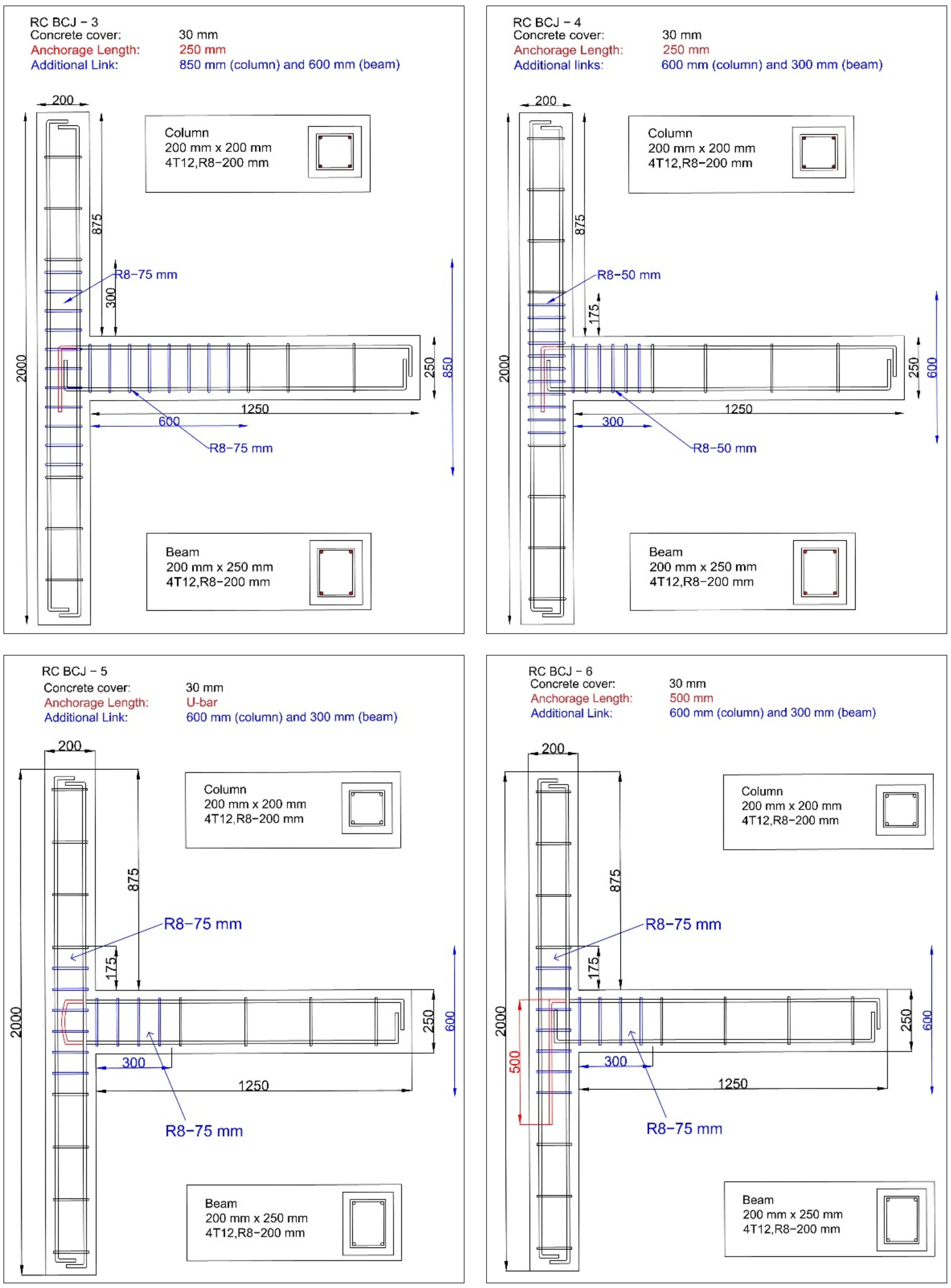
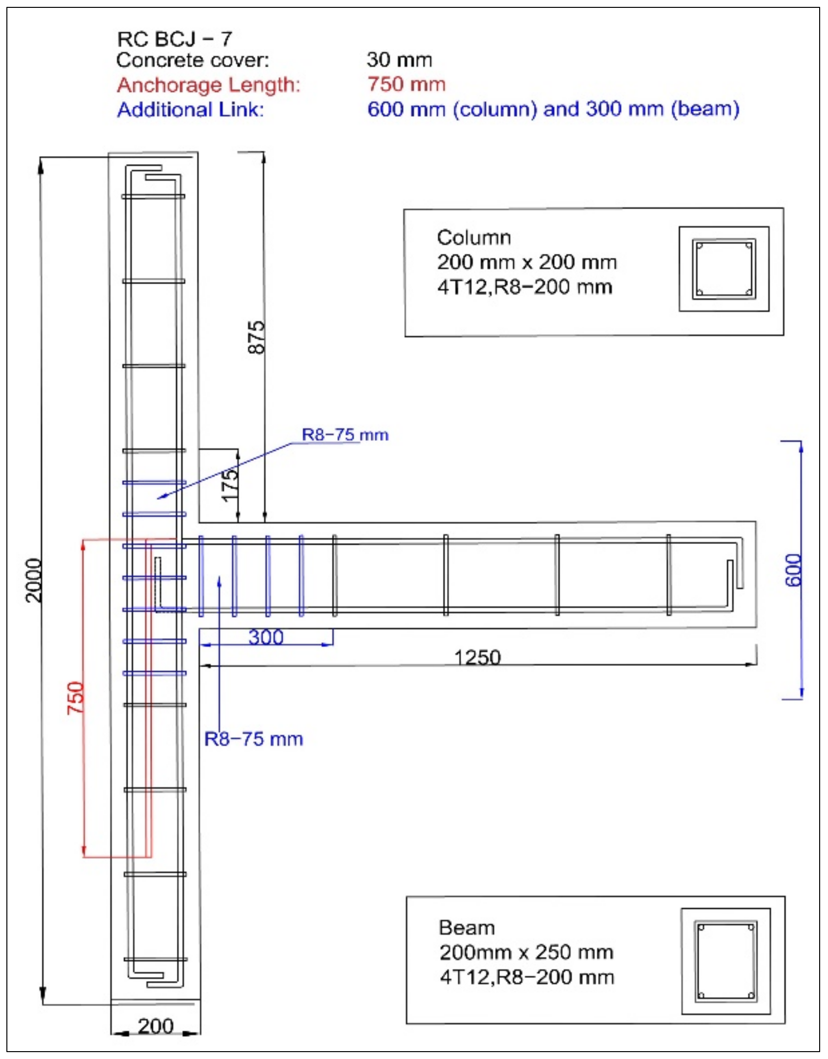
In this research, seven beam-column exterior reinforced concrete (RC) joints with a column dimension of 2000 mm × 200 mm × 200 mm and a beam dimension of 1250 mm × 200 mm × 250 mm. Type I ordinary Portland cement (OPC) obtained from Tasek 111 Corporation, Berhad, Malaysia, was used in the concrete mix design. The cement is in accordance with quality conforms 112 to EN 196. The concrete compressive strength was evaluated in accordance with the BS EN 12390-3:2009 standard [28]. Three specimens were tested for each RC beam-column joint. The average compressive strength of the cubes ranged between 41.1 MPa to 47.7 MPa. The steel reinforcement had an average tensile strength of 614.15 MPa, meeting the requirements of BS EN 10002-1:2001 standard [29]. Table 1 summarizes the reinforcement details for each RC beam-column joint. Figure 1 illustrates the reinforcement detail for each RC beam-column joint investigated. The additional shear link spacing and increased anchorage length in specimens BCJ-2 to BCJ-7 were arranged based on the ductility class medium (DCM) for low to moderate seismicity [30,31,32].
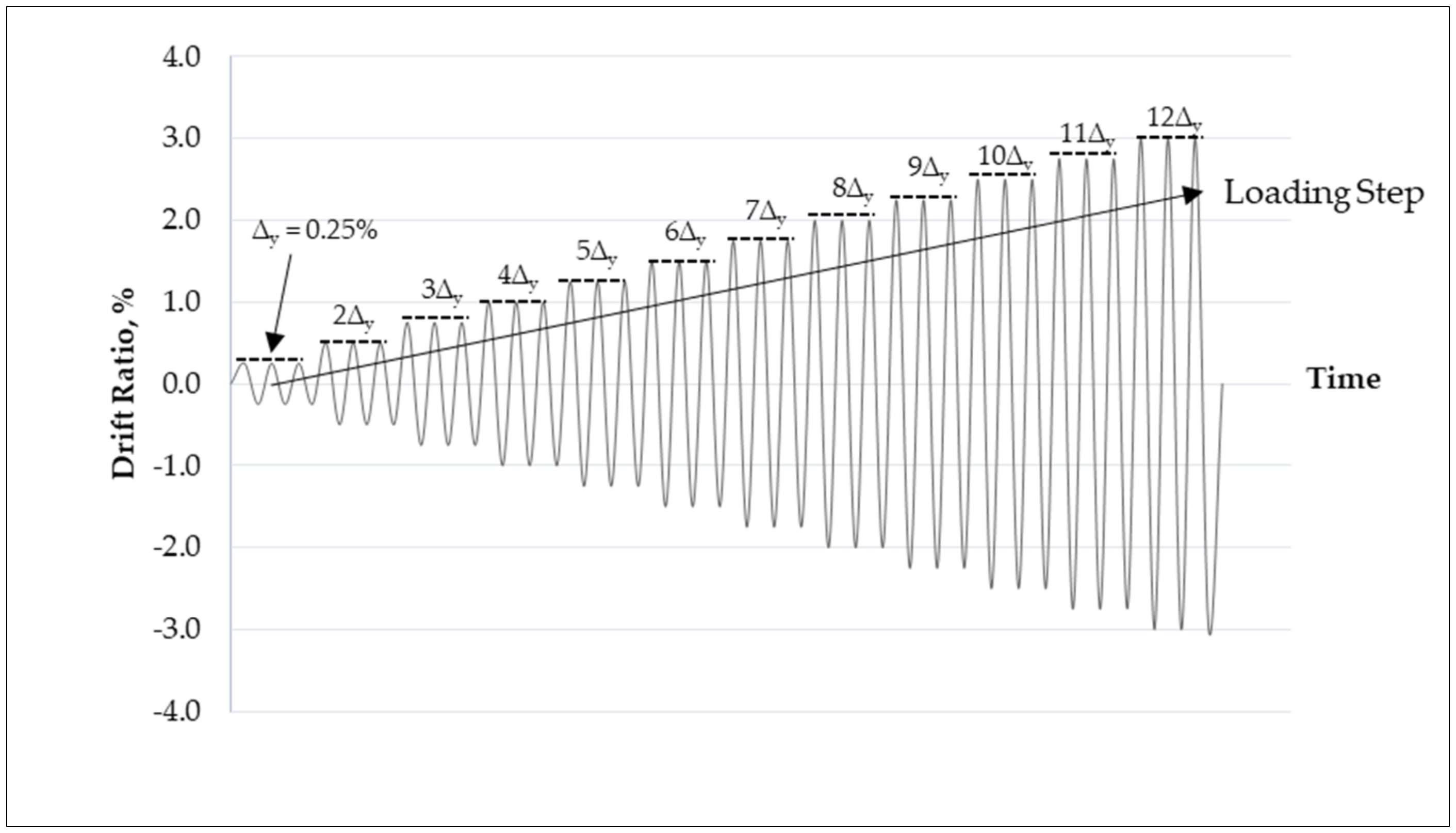
Figure 2 illustrates the schematic drawing for the experimental test setup implemented. The ends of the RC beam-column were partially fixed. A 500 kN horizontal hydraulic actuator was attached to the top portion of the column. The bottom portion of the column was braced to the surface of a strong floor. An axial circular steel pin was attached to the strong floor and the end of the beam. The specimens were experimentally tested using displacement control mode with simulated earthquake loading under lateral cyclic loading [35]. The cyclic loading history is presented in Figure 3 and is in accordance with the ACI 374.2R-13 standard [36]. Each specimen was subjected initially to cyclic loading with a drift ratio (∆y) of 0.25%. The drift ratio (∆y) was then increased by 0.25% in each step until reaching a drift ratio (∆y) of 3.00%, or specimen failure is observed. At each drift ratio (∆y) level, the specimens were subjected to three cycles. The drift ratio (∆) was defined as lx/H, where lx is the lateral movement and H is the column height [37]. Dinolite microscope camera was used to measure and analyze the crack width in every drift ratio (DR) level during testing, as recommended in earlier studies [38,39,40,41].
Table 2 illustrates the parameters recorded before and after the experimental testing that was used as potential input parameters for machine learning models to accurately predict the cracking behavior. While the crack width of each specimen represents the major output element for the prediction models.

3. Experimental Testing Results

3.1. Hysteretic Graph of Specimens

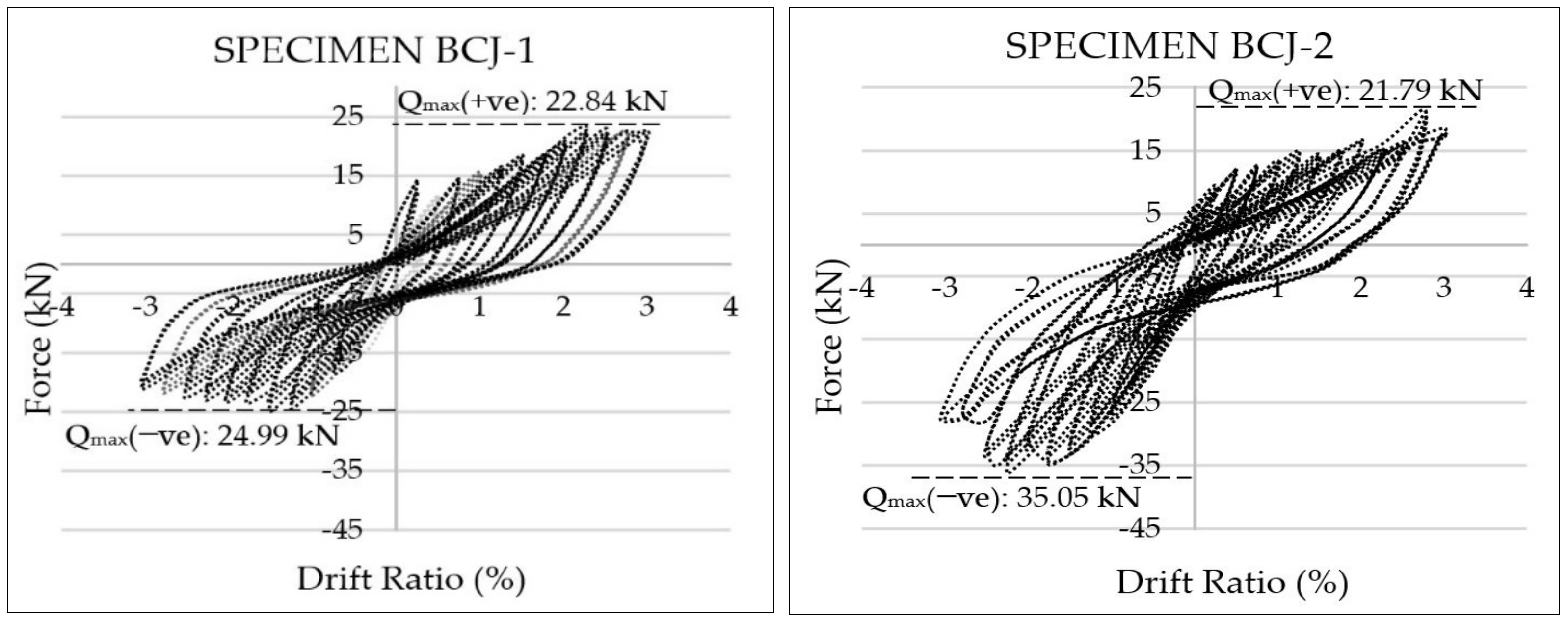
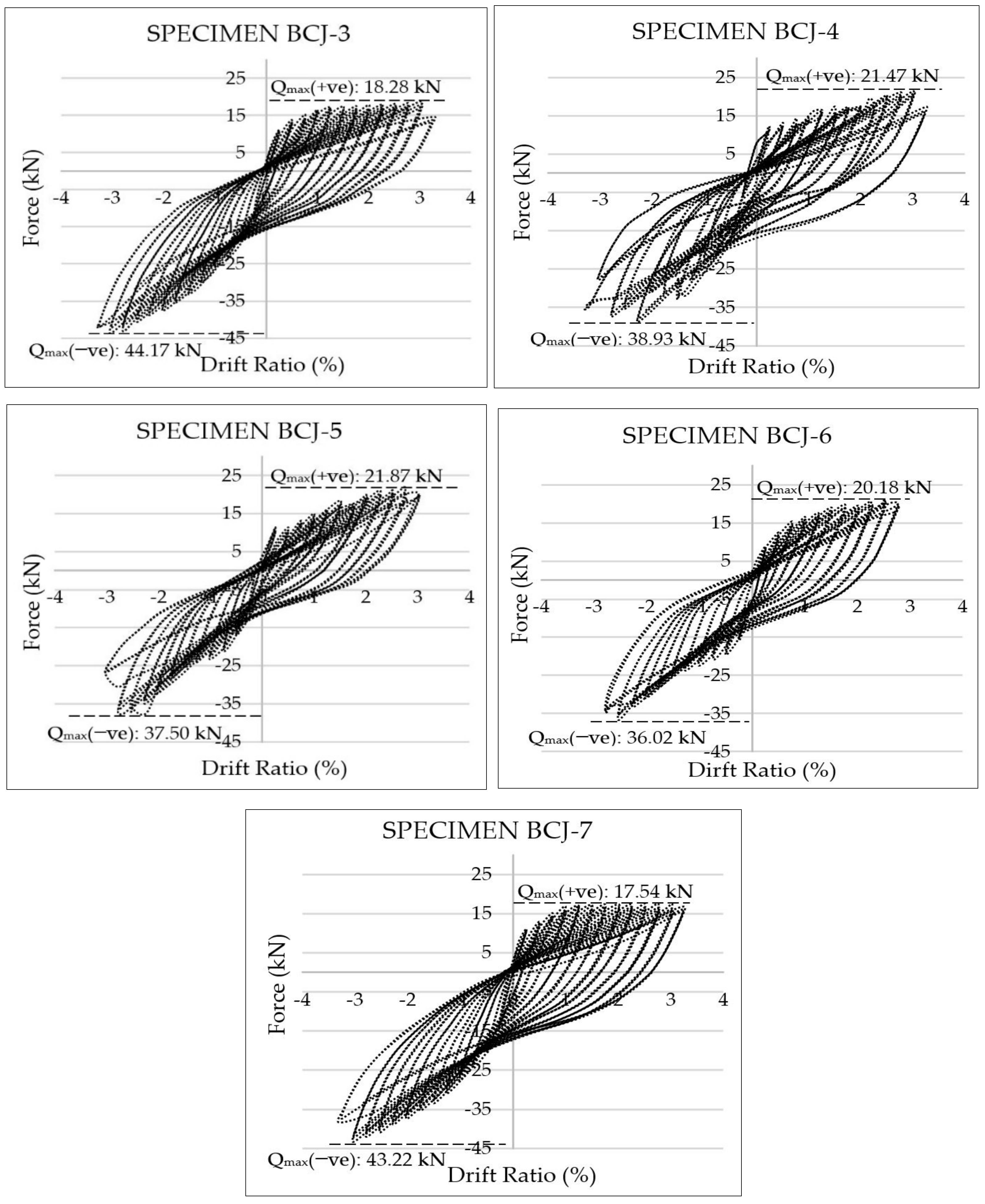
Figure 4 shows the load-drift hysteretic relationships. Qmax(+ve) and Qmax(−ve) represent the maximum positive and negative lateral load-carrying capacities of each specimen, respectively. All specimens had a greater negative lateral load-carrying capacity, i.e., Qmax(−ve), than the positive lateral load-carrying capacity, i.e., Qmax(+ve). In the case of positive Qmax(+ve), the peak load reached the maximum load-drift response (i.e., deformation capacity) at the drift ratio of 2.25% for BCJ-1, 2.50% drift ratio for BCJ-6, 2.75% drift ratio for specimens BCJ-2 and BCJ-5 and 3.00% drift ratio for specimens BCJ-3, BCJ-4, and BCJ-7. The applied displacement load for the control specimen indicated that BCJ-1 fell under tension failure mode, then the applied displacement load was forced to pull it. This resulted in the maximum negative loading obtained is similar to the maximum positive loading. This indicates that a small load is needed to pull BCJ-1 to the origin, due to low reinforcement area without any seismic strengthening provision. However, in BCJ-2 to BCJ-7, the maximum negative loadings obtained were approximately twice the maximum positive loading, compared to the control specimen. The additional shear link spacing and the increased anchorage length enhanced the strength of specimens BCJ-2 to BCJ-7.

3.2. Crack Formation of Specimens

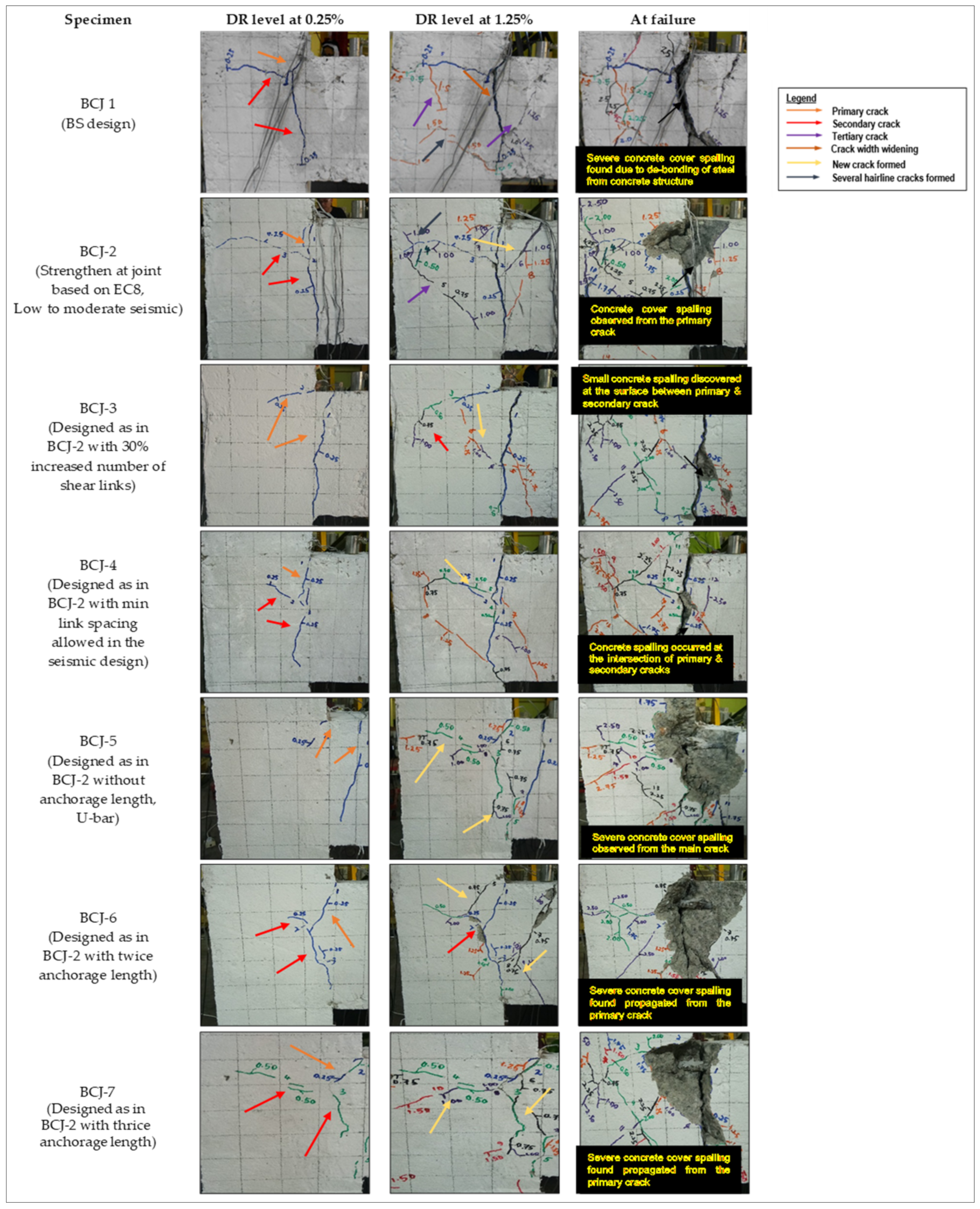
The crack pattern and width of the specimens were monitored during the lateral cyclic loading test to assess the effect of the increased number of shear links and anchorage length. Figure 5 illustrates the crack formation on the selected joint area for BCJ-1 (control), BCJ-2 (strengthen by Eurocode 8), BCJ-4 (representing additional shear links), and BCJ-5 (representing anchorage length) at the drift ratio level of 0.25%, 1.25%, and 2.25%, including at the failure. In the case of control specimen BCJ-1, the primary flexural crack initially formed at a drift ratio level of 0.25% from the top corner of the joint area and then propagated downwards to create two new secondary cracks at the intersection area between the beam and the joint panel. Moreover, numerous hairline cracks at 45° appeared at the joint interface, which extended from the primary and secondary cracks in specimen BCJ-1. For specimens BCJ-2 and BCJ-4, the primary/flexural crack was initiated at a drift ratio level of 0.25%, similar to specimen BCJ-1. However, the width and length of the crack were smaller than those of the control specimen. For BCJ-5, two primary cracks were formed at the early stage of the loading protocol. At the drift ratio level of 1.25%, a shear crack formed at 60°, and connected to the primary crack.
With repeated loading cycles, new cracks and extension of tertiary cracks increased at the joint panel zone for all specimens. The test was terminated after a drift ratio level of 3.00% for BCJ-1, due to severe crushing of concrete at the beam-column joint area. For BCJ-2 and BCJ-5, concrete cover spalling was observed at the area of primary crack beyond the drift ratio level of 3.00%. However, in BCJ-4, small concrete surface spalling was seen near the joint interfaces before failure, due to shear action beyond the drift ratio level of 3.25%. The maximum crack widths were recorded at the primary/main cracks residing at the critical zone (joint region). In general, the results indicated that the additional shear links and increased anchorage length had a significant effect on strength and on reducing the crack width.

4. The Neural Network Configuration

Artificial neural network (ANN) is an artificial intelligence modeling technique that imitates the functioning of the human nervous system. The main processing of the human nervous system consists of the brain nerve cells as the basic unit of information processing. In ANN, the basic information processing units are called neurons. Neurons manage details concurrently and immediately [42,43,44]. Implementing ANNs requires specialized building blocks, including multidimensional arrays, activation functions, and autonomous gradient computation [45]. There are many forms of neural networks, from fairly simple to very complex, just as there are many hypotheses about how biological neural processing is carried out [46,47].
Developing a structural quality model with adequate prediction accuracy can be challenging, especially when modeling the crack width of RC beam-column joints area subjected to lateral cyclic loading with respect to different levels of drift ratios. In this research, four ANN prediction models, including deep learning (DL) max-out, deep learning (DL) rectifier, support vector machine (SVM) dot, and support vector machine (SVM) neural, were used. These methods provide an optimized framework for machine learning, data mining, and text mining and are fast and easy to use [48,49,50].

4.1. Application of Deep Learning (DL) and Support Vector Machine (SVM) in Engineering Practice

Deep learning (DL) and support vector machine (SVM) are commonly used in machine learning. DL and SVM both have advantages and have performed excellently in engineering, weather prediction, stock market forecasting, and medical diagnosis [51,52,53,54,55]. DL is related to the field of machine-based learning algorithms and imitate brain neurons. DL has two main features: The ability to learn how to perform complex functions once properly trained, and the ability to generalize and establish a reasonable solution for unattended data. SVM is a computational algorithm that can learn how to allocate labels to objects from experience and examples. SVM’s fundamental function is to separate binary labeled data based on a line that achieves the maximum distance between the labeled data [56,57,58,59]. In engineering practice, DL has been applied in the fields of structural and materials engineering. Javier and co-researchers have developed a DL model for structural one-way slab design optimization [60]. The goal of this model was to reduce the environmental impact of energy consumption and CO2 emissions from construction industry operations. Improvements in slab design were explored in the model, which was able to calculate thousands of solutions in real-time based on the requirements of the designer. The authors found that the decision support system (DSS) in the model was accurate and presented multi-criteria solutions that significantly reduced emissions without affecting the cost. Another related DL model was built to measure the local health of structures by establishing the Structural Health Index (SHI) [53]. Ambient noises have been applied to the SHI model to replicate the structure’s damage rate. A comparison of vibration records from a 1:20-scale residential 42-story high-rise concrete building in Hong Kong with the degree and magnitude of damages obtained from SHI modeling verified the capability of the model. The authors proposed that this model could also be extended to systems for informed and warning maintenance decision-making for both local and global real-time health monitoring. Research on the development of instance-level identification and quantification of concrete surface bug-holes, based on DL was carried out [61]. The authors posited that this model was necessary to avoid the conventional, time-consuming, and inefficient methods of measurement performed by manual inspection. Hence, a total of 428 raw images with the appropriate bug-hole resolution were chosen to create the datasets, and the result showed that the model achieved an average accuracy of more than 90% of the quantification defects with real concrete surface bug-hole specimens compared to traditional CNN models. The authors recommended this model for future time-saving inspection, while avoiding applying the traditional CNN model that was inefficient in the accurate location of defect boundaries that led to difficulty in quantifying defects.
For the SVM model, the compressive strength and prediction of autogenous shrinkage for concrete were developed, respectively, using the regression technique [62,63]. One of the distinguishing features of SVM is its limited number of parameters compared to other types of prediction models that need a design that must integrate network structure and be combined with powerful optimization algorithms to deliver satisfactory results [64]. In these researches, both authors [62,63] applied five and nine numbers of parameters, respectively, to further simulate and correlate the predicted outcome with the experimental results. In both cases, the SVM predictions were in relatively good alignment with the findings observed. In addition, the accuracies of the proposed SVM models were compared with predictive models based on ANN. The predictive models based on ANN showed a higher R2 value than the SVM models, suggesting that SVM’s predictive efficiency is comparable to ANN. Nevertheless, the authors indicated that ANN models require a large number of optimization control parameters and a relatively large training database, while SVM requires few control parameters with little reliance on the size of training datasets. SVM proposed this benefit as a viable alternative to other ANN methods. In addition, the SVM-based classification was established to detect horizontal subsurface cracks in the pavement to avoid shortening the lifespan of roadways [65]. The model was added with the root-mean square error (RMSE) performance index to avoid over-fitting in positive identification. The predicted classification results were then compared with the standard reference method Amplitude Ratio Test (ART). The comparison indicated that SVM was efficient in the detection of de-bonding within pavement structures. Sensitivity analysis was included and further carried out using various parameters to obtain the robustness of SVM. It was found that SVM distinguished the composite structures implemented in pavement structure de-bonding with greater accuracy. Hence, the robustness of the SVM method had increased the potential in the detection process. Amin and Farhad showed that SVM-based reliability analysis of concrete dams can predict flood assessment of gravity dams and optimal earthquake intensity. They compared their results to those obtained using finite element method analysis (FEM) [66]. The authors determined that SVM has a lower computational cost when compared to FEM-based probabilistic simulations. Furthermore, each of the nonlinear transient time history analyses and its post-processing (in the second example) takes 10–25 h (depending on the period of the ground movement and the degree of damage) for FEM. Hence, a complete set of 100 analyses would require a computation time of about two months compared to the runtime of a few hours of an SVM model. Consequently, the authors stated that SVM is a useful and effective method for the classification, prediction of response, and reliability analysis of concrete dams.

4.2. Framework Model of Deep Learning (DL) and Support Vector Machine (SVM)

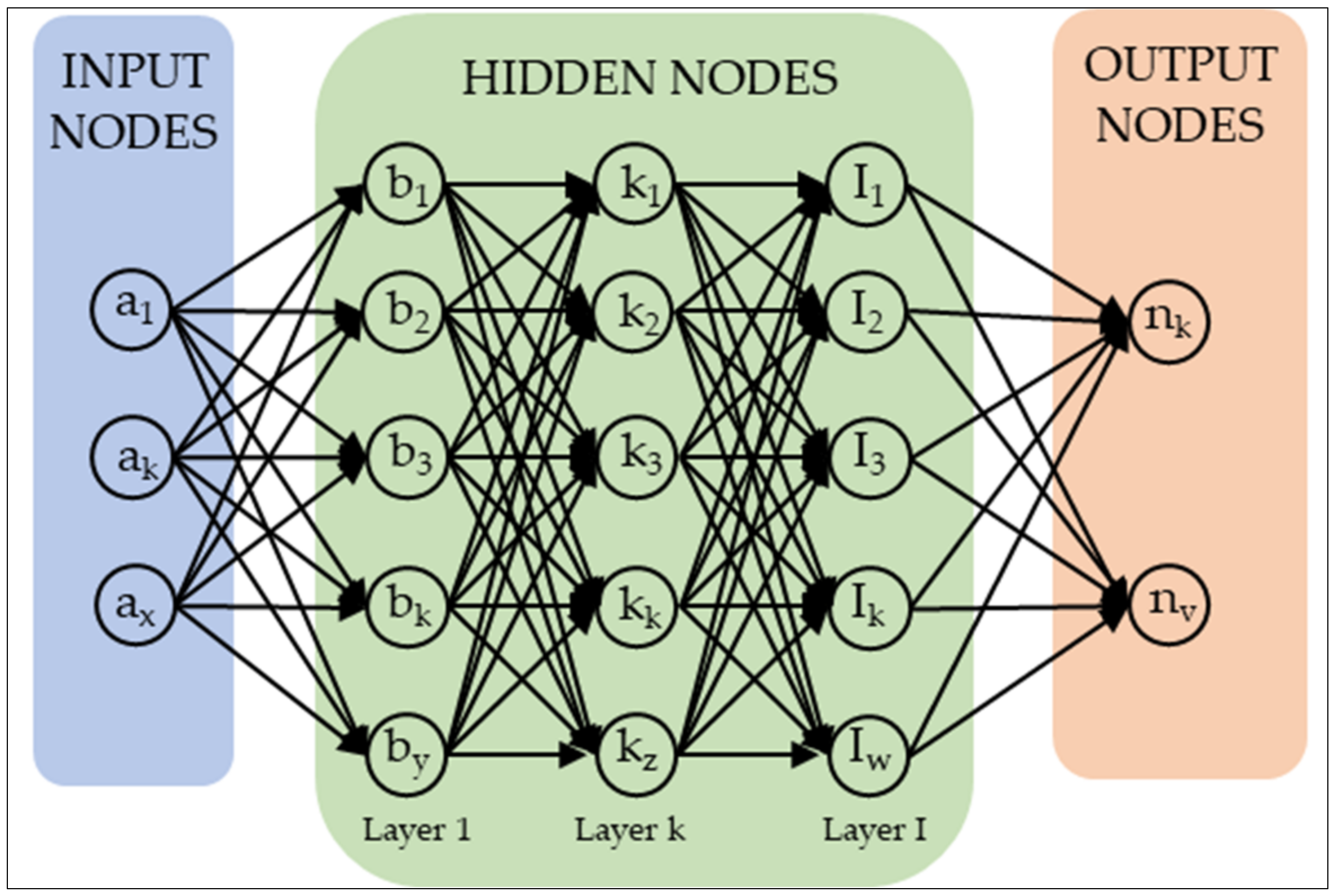
The basic framework of ANN requires three layers (Input, Hidden, and Output) [67], as shown in Figure 6. The input layer is the first layer where data/features are obtained, and some standardization techniques are used to restrict inputs to a certain set. The structured inputs make the neural network work easier, resulting in better accuracy. Depending on the network application, the hidden layer (intermediate or invisible) may be a collection of layers. Such layers are responsible for identifying the pattern of a process or device. Most operations of the neural network are carried out in these layers. The output layer also contains neurons representing the outputs of the final network generated from the previous layers of neuron processing. The basics of ANN’s composition involve neuronal interconnection and layer formation. Therefore, they may categorize their temperament into four different types. Such types include feed-forward single-layer, mesh, recurrent, and feed-forward multi-layer networks.
DL is a class of machine learning algorithms that slowly extract higher-level features from the raw input using multiple layers. For example, lower layers can identify edges in image processing, whereas higher layers can identify human-relevant concepts, such as digits, letters, or faces [56]. The term ‘DL’ was introduced by Rina Dechter in 1986 [68,69], then followed by Igor Aizenberg and his colleagues in 2000 in the form of Boolean threshold neurons [70,71]. The hidden layers (see Figure 7) perform complex mathematical computations based on the number of inputs. The disadvantages of the DL model include the requirements of a large dataset and large amounts of computational power in both training and testing [72].
The concept of SVM was originated and developed by Cortes and Vapnik [75] to introduce a classifier derived from the theory of statistical learning. It has since been shown to be very robust, and also has been used as an intuitive model representation to detect outliers. SVM is a supervised technique in machine learning used for problems of classification, as well as regression. Even with few examples, SVM performs well and has good accuracy. Because of these benefits, SVM differs from other techniques of machine learning [75,76,77]. In addition, the following order provides a brief description of the principles of SVM [78]. SVM’s goal is to find a function f that has a maximum ε deviation from the actual targets xn for all the training data, and is as flat as possible. The functions f can be represented by the following equation for the training data:
f x = ω , x + b
where ω < X and b < R; <, > refers to the dot product in X; ω is the weight vector; b is the scalar threshold. SVM determines the regression function in accordance with statistical theory by minimizing an objective function. The regression function parameters x and b are calculated by minimizing the regularized function of risk as follows:
1 2 ω 2 + C i = 1 n ξ i + ξ i *
Subject to,
y i ω , φ x b     ε + ξ i ω , φ x + b y i     ε + ξ i * ξ i ,   ξ i *   0 ,   i = 1 , 2 n
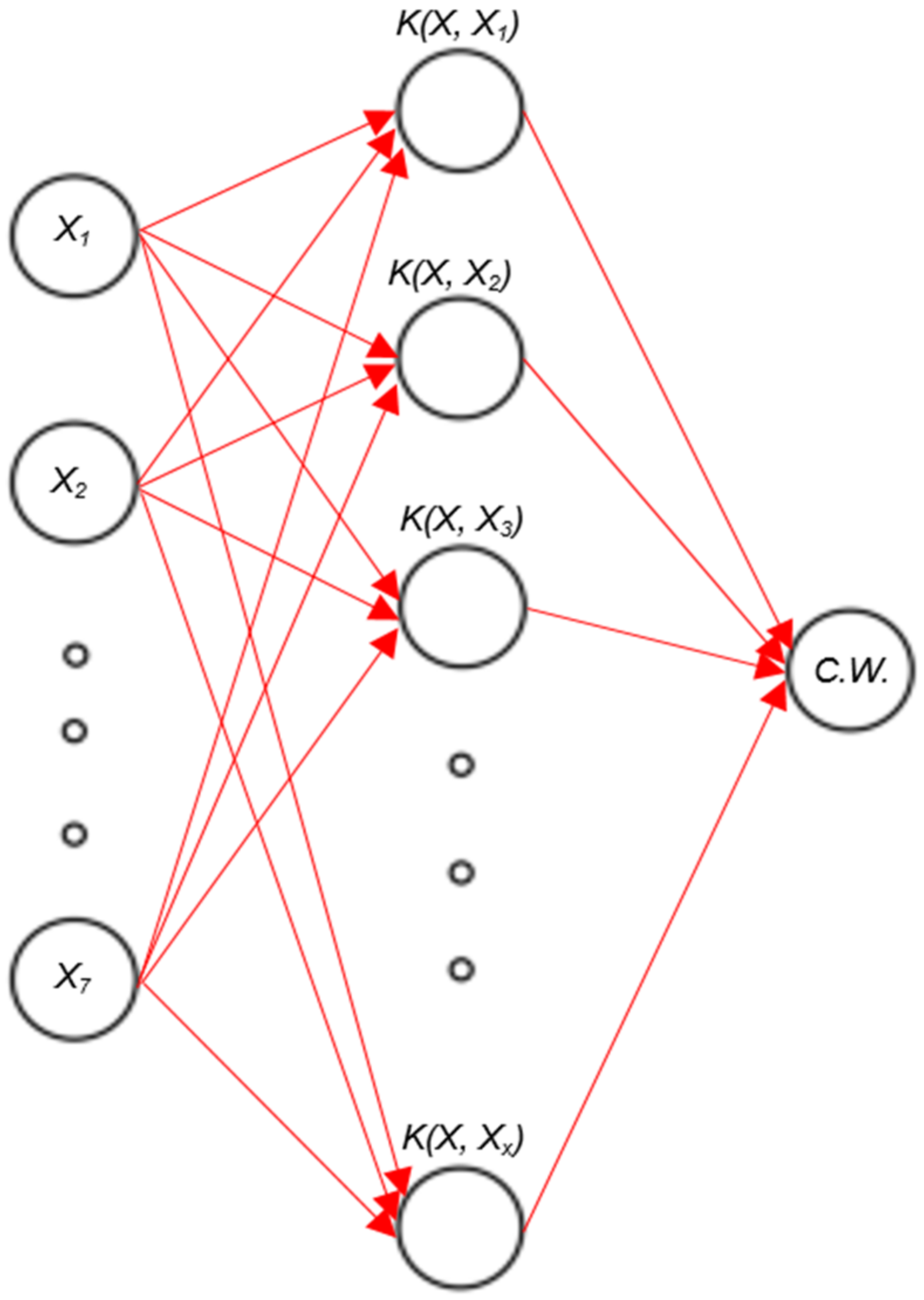
where C is the pre-specified SVM tolerance parameter, ξ i and ξ i * are slack variables in determining the degree to which data points will be penalized if the error is larger than precision parameter ε . ε is the insensitive loss function. The SVM training algorithm will rely only on the data in high-dimensional space via dot products. In addition, the kernel function generated in Rapidminer can be used to approach the dot products in high-feature dimension space as in Equation (4) and in Figure 8, we only need to use K in the SVM training algorithm without specifically treating the function space to obtain the specific formulation of the algorithm of . The kernel parameters must be carefully selected because they are important to define the high-dimensional space and to monitor the complexity of the final solution. Because SVMs are primarily defined by the types of their kernel functions, it is important to choose the correct kernel function and kernel parameters for each application problem to ensure satisfactory results. A trial-and-error technique was used to pick the kernel-specific parameters.
K x i , x n = <   x i ,     x n
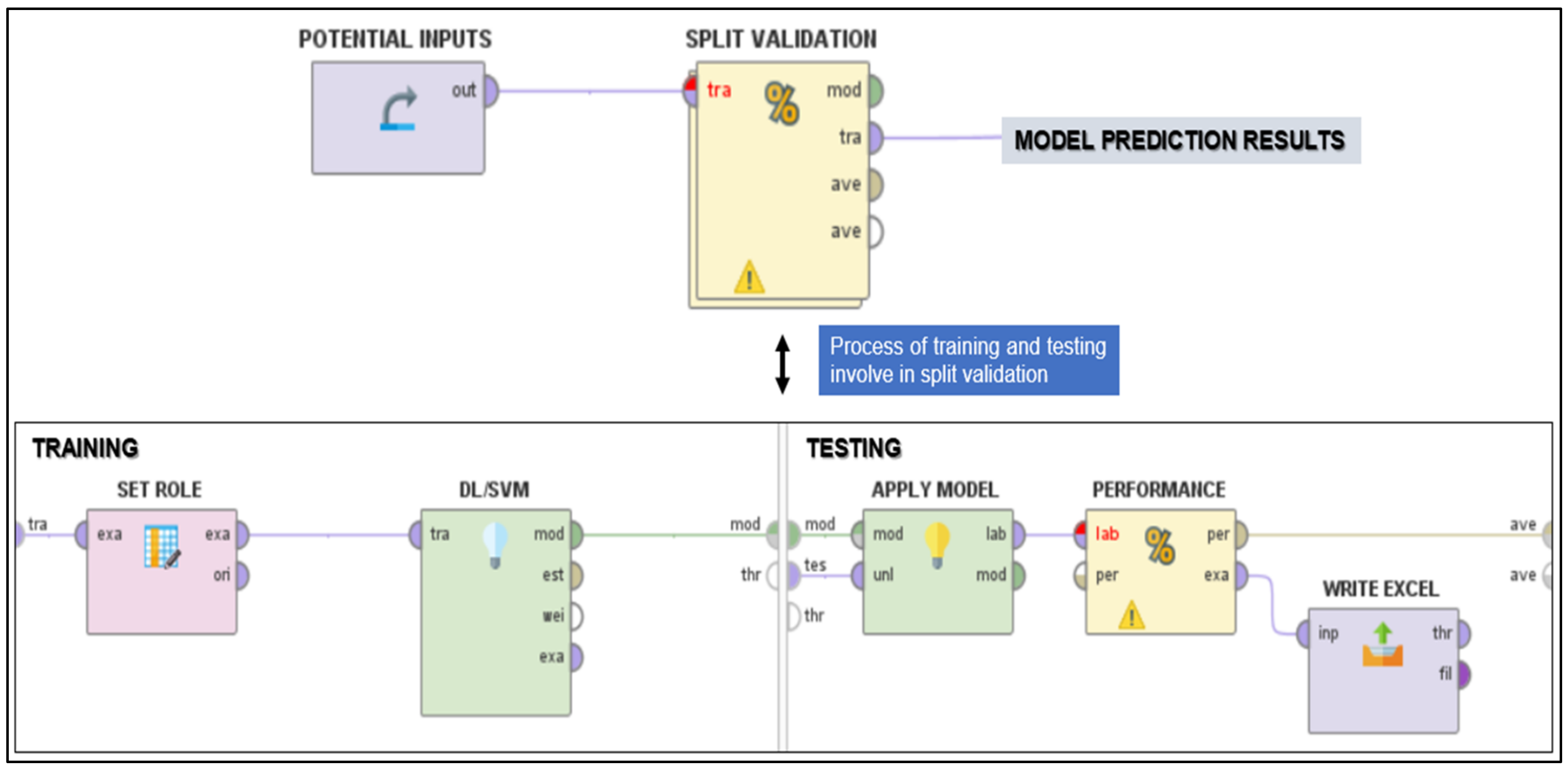
In this research, the framework model was used, as illustrated in Figure 9. The regression performances of classification for all models were evaluated by the labeling dataset, where the inputs data were attributed with label roles, while an attribute with prediction role for experimental crack width data. The attribute of the label stores the real observed values, while the attribute of prediction stores the label values expected by the regression models. Training with a collection of sample data called a training set generates the models. Trained models were then provided with the test set to predict the accessible accuracy of data on crack widths. For the simulation, nine numbers of potential inputs vectors were selected, and a split data ratio of 75:25 (training set to test set ratio) was applied for all prediction models. The prediction models are described further in the following Section 5.1.

5. Results and Discussion

5.1. Comparison of Prediction Models from Rapidminer

A sufficient list of numbers (≤1000 data) of crack width data of seven RC beam-column joints was collected at every respective drift ratio level. The data were used for training and testing in the Rapidminer software based on the recommendations from literature as described in Section 4.1 [66]. Four different prediction models were developed and proposed as defined in Table 3 with potential input parameters.
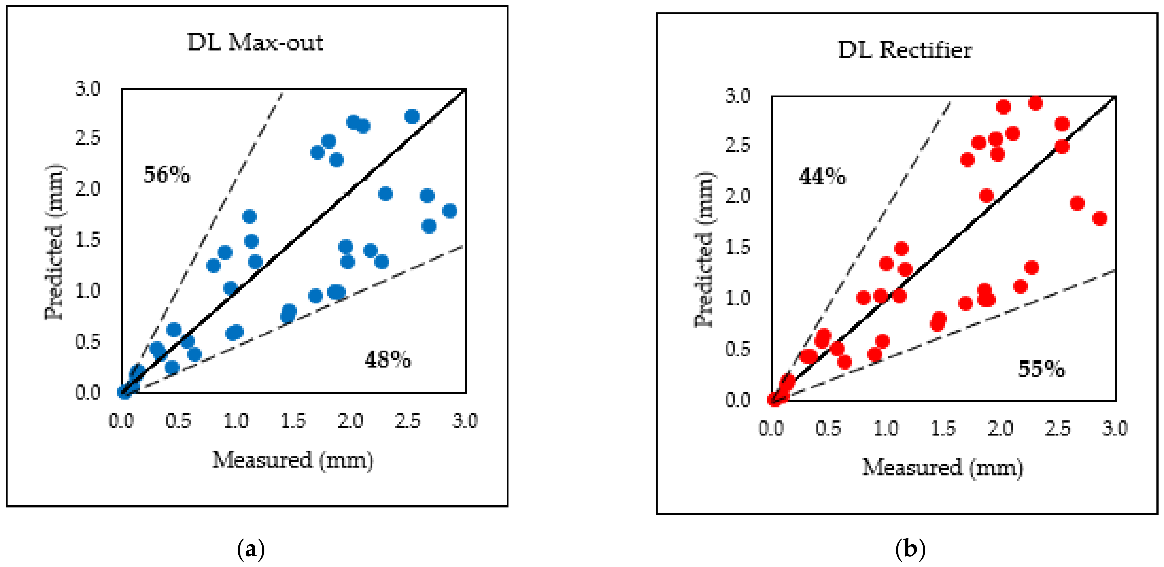
Figure 10 illustrates regression analysis plots for the distribution of predicted crack width. The figure includes the equity line as a guide, which for the predicted and measured crack widths reflects the state of equal value. The analysis shows that SVM model with dot prediction method presented better prediction with the smallest error, in which the distribution of predicted was below (27% error) and above (30% error) of the reference line compared to DL max-out (48% and 56%), DL rectifier (55% and 44%) and SVM—neural (29% and 48%). DL max-out and DL rectifier showed that almost all predicted points were distributed around the measured crack widths with the largest errors, due to over-fitting. These observed errors might be attributed to insufficient data as DL models require a large dataset for complex supported calculation/simulations [61,72]. The accuracy of predicted crack widths by SVM—dot was consistently increased within equity line, thus demonstrating regression technique with input-output relationships. This was further supported by the regression technique developed for compressive strength and predicting autogenous shrinkage for concrete [62,63]. Hence, in the field of machine learning, SVM is the best learning methodology for classification and regression tasks [79,80,81]. Though the SVM—neural showed a difference of 2%–18% from SVM—dot, however homogenous floats formed on top linear measured line at the area with more than 1.5 mm have shown uncorrelated and over-predicted values between the predicted and actual crack widths. Therefore, the SVM—dot model was selected for further analysis of optimization using data splitting, numbers of input parameters, and performance index and is described in the following sub-section.

5.2. Data Splitting Ratio Analysis in SVM—Dot Model

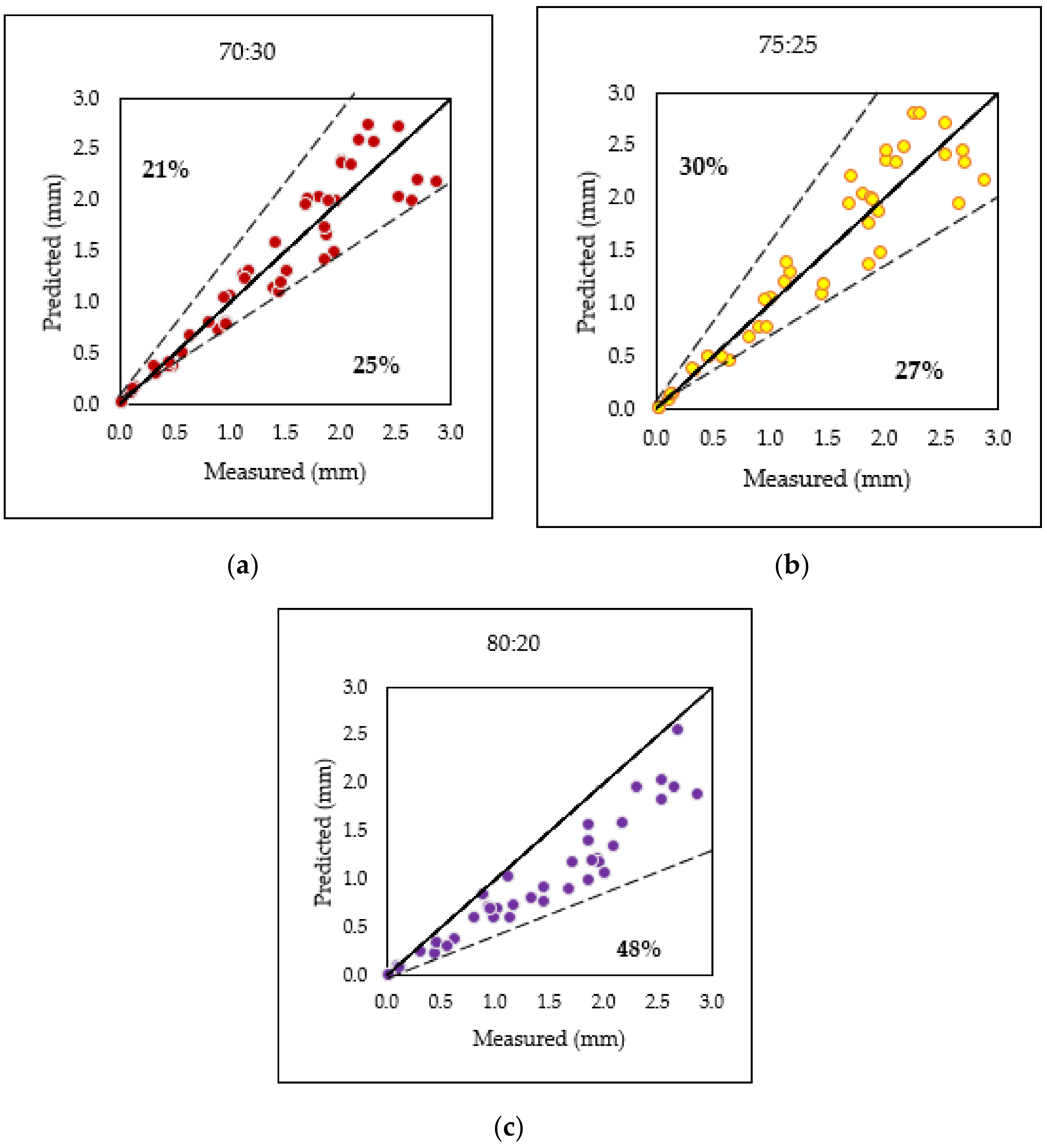
One of the most important decisions to be made when developing a prediction model is to make full use of existing experimental data to optimize the prediction model. The most common technique is to divide the data into two—typically referred to as the sets of training and testing. The training set is used to build models and is used as the substratum feature set to estimate parameters, compare models, and all other activities necessary to develop a complete model. The test collection is applied to determine the final and objective evaluation only at the end of these activities. Before this point, it is important that the test set is not used. Looking at the results of the test sets would skew the results because the test data were part of the process of model creation. Improper splitting of the dataset will result in the output of the model being excessively high. Nonetheless, various sophisticated methods of sampling were used to address this problem. In addition, an important aspect of data splitting is how well the training, testing, and validation datasets describe the feature space when the number of points in the whole dataset is large during when any division ratio would work, but when the dataset is limited, division ratio may play a crucial role [82,83,84]. The SVM—dot model from Section 5.1, is selected for further analysis. When a specific test set was not available, the split validation operator was implemented to predict the model’s fit to a hypothetical test set. The split validation operator can also train on one set of data and check on another set of specific test data. The purpose of splitting data into two different categories in this prediction model was to avoid over- and under-fitting and only optimizing the training dataset accuracy. Hence, there is a need for a model that performs well on a dataset that it has never seen (test data), which is called generalization. In this case, the training data and test data are contributed randomly by seven specimens (not from the same specimen) with different detailing, load-carrying capacity, different maximum drift ratio, etc. The test data and training data from every specimen are independent from each other as they have different designs. This procedure has assured the pattern of input-output data during the testing is different than the pattern used during the training. Figure 11 shows three different results based on linear sampling for the split ratio between training and testing of 70:30, 75:25, and 80:20 from the prediction model.
Results show that the split ratio of 70:30 with the lowest error of predicted crack widths (25%) near the reference line. It is, thus, a better split ratio for the SVM—dot than 75:25 (30%) and 80:20 (48%) of split ratios. Most of the plotted predicted points for the 80:20 split ratio were far below the equity/measured line, due to unbalanced data from a smaller number of datasets, thus, providing high variance in prediction, which can significantly change testing accuracy. In other words, significant under-fitting in the 80:20 split ratio may cause redundancy in experimental output data. Past studies have shown that the proportion chosen in the analysis for fewer numbers of datasets (≤1000 data) was 70% for the training set and 30% for the test. The idea is that more training data is preferred because it makes the classification and regression models better, whilst more test data makes the error estimate less accurate [85,86,87]. For this dataset, the 70:30 split is within this experimental range and is a reasonable choice. The trade-off is simple as less the testing data, bigger the variance performance of the model algorithm, while more the training data, smaller would be the variance in parameter estimates. From this 70:30 split ratio graph, further optimizations are analyzed and discussed based on the number of input parameters selected in the following sub-section.

5.3. Analysis on Input Parameters Selection for SVM—Dot Model

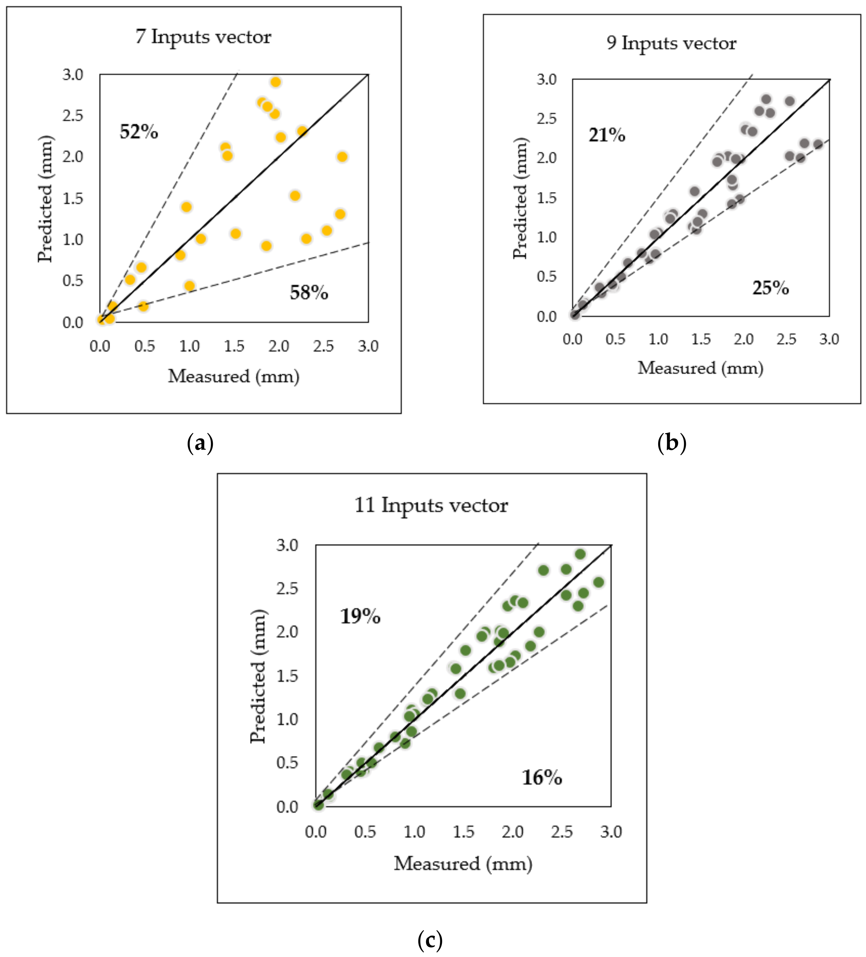
To define the optimal functional type of regression models, the choice of input variables is central and crucial. The role of selecting input variables is common to the creation of most models of regression and depends on the discovery of relationships within the available data to identify acceptable model output predictors. The difficulty of the input variable selection task is somewhat alleviated in the case of parametric or semi-parametric empirical models by a-priori assumption of the model’s functional form, which is based on some physical interpretation of the underlying system or process being modeled. In the case of ANN, however, there is no such inference about the model’s structure. The input variables are instead chosen from the available data, and the model is subsequently developed [88]. Consequently, three different types of input variables are used, as seen in Table 4, to integrate flexibility and prevent duplication, providing a more reliable model of prediction. The results for variable input vectors in determining the correlation and consistency between predicted and measured crack widths are presented in Figure 12.
Several important parameters that were omitted for seven inputs resulted in over-fitting (52–58%), due to the discrepancy of data between predicted and measured crack widths. The smaller number in sample size with the smaller number of inputs does not effectively cover the prediction observed in the broader domain. This can seen in Figure 12a, where a large variance developed in the regression model based on the smaller number of inputs dataset. As seen in Figure 12b, the load parameter (Qmax(+ve) and Qmax(−ve)) played a significant role, thus showing how important the parameters are correlated in engineering terms to approach with experimental crack widths data. Even though the prediction model with nine inputs was sufficient (21–25% difference between measured to predicted), however in contrast to previous studies [63,65], Figure 12c with additional concrete tensile strength (Ct) and reinforcement tensile strength (Tt) had proved that the smaller number of datasets with an increased number of inter-related inputs parameter had drawn back less than 20% consistency of predicted points varied and equally within above and under the reference lines. Several studies found it difficult to pick input variables because of the number of variables available; associations between possible input variables will establish overlap and variables with little or no predictive power [89,90]. The redundancy occurred depend on the kind of ANN model used followed by the numbers of performance operators needed for complex analysis compared to SVM. A dot model was applied in this study whereby fewer operators were used, as in Figure 10, with straight-forward analysis, which was highly suitable for smaller number of datasets—thus developing a more robust and efficient regression model. Further analyses and modifications are made for the predictive model, based on Figure 12c, where the additional operator, performance index, is applied, as described in the following sub-section.

5.4. Analysis on Performance Indexes (Regression) Supported in SVM—Dot Model

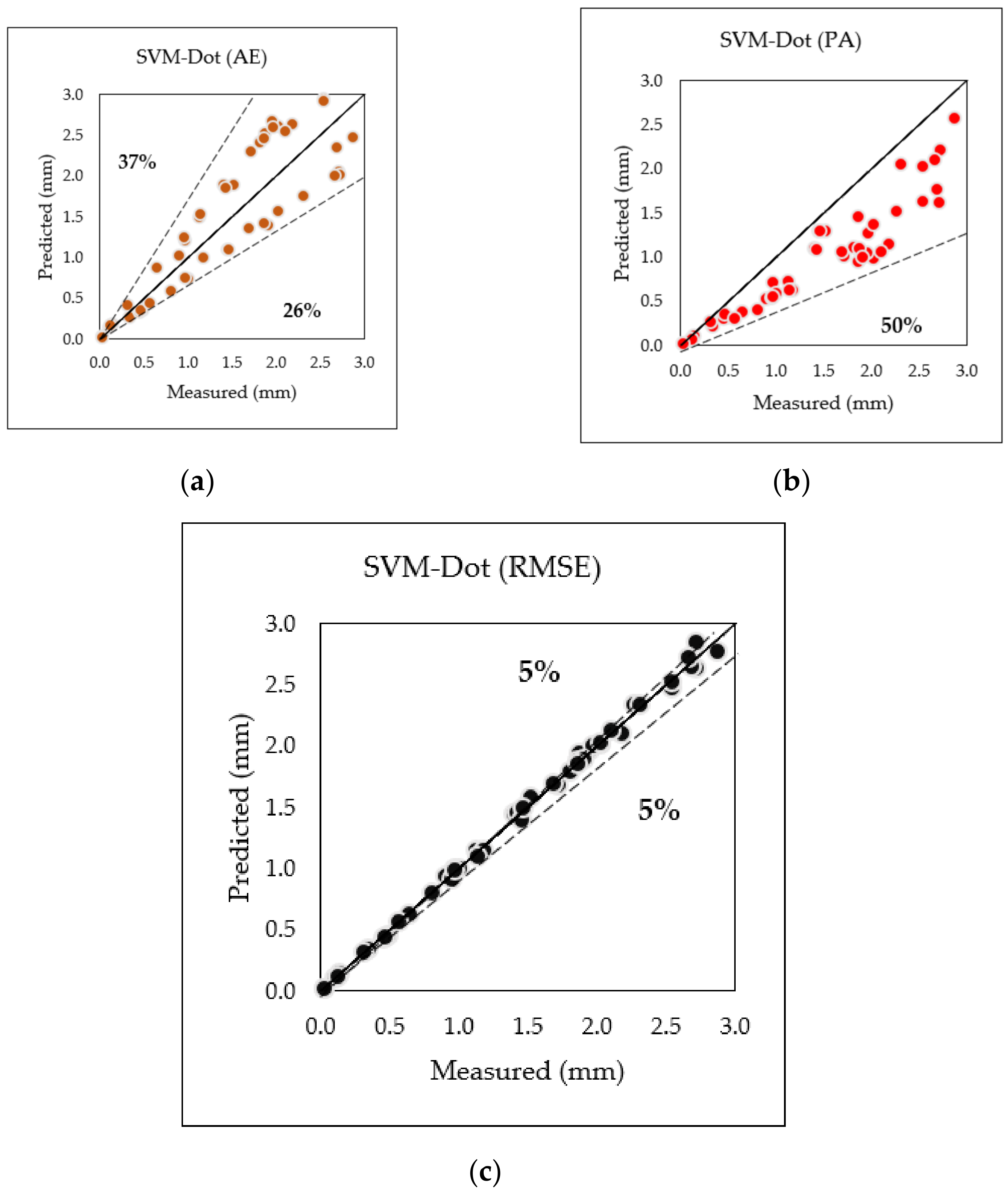
Performance index operators were used to test the regression task with statistical performance and provided a list of the regression task’s accuracy criteria values. The operator output (regression) was selected as it decides the type of learning task and measures the most common requirements for that category automatically. Regression operation is also a method used for numerical analysis and is a statistical measure that evaluates the intensity of the relationship between a dependent variable (label attribute) and a set of other changing variables known as independent variables (regular attributes). This type of operator has been constantly used in previous studies to evaluate specific factors, such as commodity price, interest rates, and certain industries, that affect the price movement of an asset [91,92,93]. To evaluate the statistical efficiency of the regression model, the dataset must be labeled and must have a label function attribute and a predictive role attribute. The attribute of the label stores the actual observed values, and the attribute of the prediction stores the label values predicted by the regression model under discussion. For this research, three types of index regression (as in Table 5) were used to refine and reduce the difference/gap between measured and predicted crack widths, and are shown in Figure 13.
From the above figure, RMSE can be seen to exhibit a more consistent standard deviation of residuals (prediction errors) up to 5%, approaching actual crack widths compared to AE (26–37%) and PA (50%). The inconsistent prediction performance was found over-fitting in the case of AE and under-fitting in the case of PA from the reference lines, respectively. The extent of error found in the prediction model associated with AE and PA may be considered from the point of view of accuracy. The accuracy of measurement reflects the error or variance of the measurement from the average of a large number of measurements of the same quantity, whereas the precision of a measured value expresses the deviation of the measurement from the real quantity value. Error is viewed from the point of view of precision when the true value is known, but it must be used instead of accuracy when the true value of a quantity is not known. Accuracy cannot be achieved if the precision cannot be reached; however, precision does not guarantee accuracy. Residuals were calculated as to how far the data points were from the regression line; RMSE was assessed as to how these residuals were spread out. In other words, it shows how clustered the data is around the best fit axis, thus supporting the argument through a previous study in which RMSE was able to avoid over-fitting in positive identification [62,65]. This parameter of the RMSE index is, therefore, a simple, quick, and reliable metric compared to other parameters, widely used in climate analysis, forecasting, and regression to validate experimental results [50,64,94].

6. Conclusions

In this research, prediction models were developed to analyze and predict crack width in reinforced concrete beam-column joints area subjected to lateral cyclic loadings. The prediction models were developed considering the cracks observed at each drift ratio level with numbers of additional shear links and length of the anchorage within the joint region using Rapidminer machine learning tools. The results have shown that the support vector machine (SVM) model can provide accurate and precise performance on the crack widths prediction process. The following conclusions are drawn in this study:
  • SVM—dot kernel prediction model exhibited 30% fewer discrepancy values between measured and predicted crack width compared to DL—max-out (56%), DL—rectifier (55%), and SVM—neural (48%) and was therefore chosen.
  • For the data splitting ratio, 70:30 split of testing and training smaller number dataset was comparable to the experimental range, thus being a decent and reasonable choice in this research.
  • The higher number of input variables (eleven inputs) being pre-processed by the SVM—dot model was recommended, where the small dataset for this research with an increased number of inter-related inputs parameter presented errors less than 20% consistency of predicted points varied along the reference lines compared to over-fitting result found in seven inputs (52–58%) and less under-fit found in nine inputs (21–25%), respectively.
  • Finally, based on conclusion (2) and (3), further optimization was made where the root mean square error (RMSE) performance index was adapted, and the SVM—dot prediction model further reduced the error between measured and predicted crack width up to 5% compared to absolute error (AE), 37%, and prediction average (PA), 50%, respectively.
Although the proposed model uses SVM—dot with RMSE optimization, it has been proven to provide a reliable accuracy for the current application. However, it is only applicable for the lateral cyclic loading, which simulating the earthquake loading, as this is the main scope of the study. In the case for the different types of RC material or loading programs, the new dataset is required to improve the model, which may be considered for future work.

Author Contributions

Conceptualization, methodology and project administration, R.G., C.G.T. and A.E.-S.; software, R.G. and A.E.-S.; validation, R.G., A.E.-S. and Z.I.; formal analysis, data curation and writing—original draft preparation, R.G.; investigation, R.G. and C.G.T.; resources, R.G., C.G.T., A.E.-S. and Z.I.; writing—review and editing, M.M.S. and F.M.N.; visualization, R.G., F.M.N. and A.E.-S.; supervision, C.G.T., Z.I. and A.E.-S.; funding acquisition, C.G.T., A.E.-S. and M.M.S. All authors have read and agreed to the published version of the manuscript.

Funding

Supported by University of Malaya RU Grant—Faculty Program (GPF007A-2019).

Institutional Review Board Statement

Not applicable.

Informed Consent Statement

Not applicable.

Data Availability Statement

The experimental results were taken and cited from author’s own paper (in press); https://doi.org/10.1139/cjce-2019-0578 (accessed on 30 October 2020).

Acknowledgments

This study was supported by the Research Fund Assistance from the University of Malaya under RU Grant—Faculty Program (GPF007A-2019). The author thanks the Universiti Tun Hussein Onn Malaysia for providing scholarship under S.T.A.B scheme (2017) to perform this work.

Conflicts of Interest

The authors declare no conflict of interest.

References

  1. Elshafey, A.A.; Dawood, N.; Marzouk, H.; Haddara, M. Crack width in concrete using artificial neural networks. Eng. Struct. 2013, 52, 676–686. [Google Scholar] [CrossRef]
  2. Allam, S.M.; Shoukry, M.S.; Rashad, G.E.; Hassan, A.S. Crack width evaluation for flexural RC members. Alex. Eng. J. 2012, 51, 211–220. [Google Scholar] [CrossRef] [Green Version]
  3. Pancic, A.; Milasinovica, D.D.; Golesb, D. Crack propagation in flexural fatigue of concrete using rheological-dynamical theory. Comput. Concr. 2021, 27, 055. [Google Scholar]
  4. Haeri, H.; Sarfarazi, V.; Zhu, Z. Effect of normal load on the crack propagation from pre-existing joints using Particle Flow Code (PFC). Comput. Concr. 2017, 19, 99–110. [Google Scholar] [CrossRef]
  5. Haeri, H.; Sarfarazi, V.; Shemirani, A.B. Experimental and numerical study of shear crack propagation in concrete specimens. Comput Concr. 2017, 20, 57–63. [Google Scholar]
  6. Hull, D. Fractography: Observing, Measuring and Interpreting Fracture Surface Topography; Cambridge University Press: Cambridge, UK, 1999. [Google Scholar]
  7. Shah, S.P. Size-effect method for determining fracture energy and process zone size of concrete. Mater. Struct. 1990, 23, 461. [Google Scholar] [CrossRef]
  8. Souza, J.C. What Do the Cracks in Concrete Structures Mean? Available online: https://www.archdaily.com/879953/what-do-the-cracks-in-concrete-structures-mean/ (accessed on 28 July 2019).
  9. British Standards Institution. BS 8110-2: 1985: Structural Use of Concrete—Part 2: Code of Practice for Special Circumstances; British Standards Institution: London, UK, 1985. [Google Scholar]
  10. ACI. ACI 224R-01: Control of Cracking in Concrete Structures; American Concrete Institute: Farmington Hills, MI, USA, 2001. [Google Scholar]
  11. Normalisation, C.E. Eurocode 2: Design of Concrete Structures: Part 1-1: General Rules and Rules for Buildings; British Standards Institution: London, UK, 2004. [Google Scholar]
  12. Shinmura, A.; Saouma, V.E. Fluid fracture interaction in pressurized reinforced concrete vessels. Mater. Struct. 1997, 30, 72–80. [Google Scholar] [CrossRef]
  13. Goszczyńska, B.; Trąmpczyński, W.; Tworzewska, J. Analysis of Crack Width Development in Reinforced Concrete Beams. Materials 2021, 14, 3043. [Google Scholar] [CrossRef] [PubMed]
  14. Beeby, A.W. The influence of the parameter ϕ/ρ eff on crack widths. Struct. Concr. 2005, 6, 155–165. [Google Scholar] [CrossRef] [Green Version]
  15. Edwards, A.D.; Picard, A. Theory of cracking in concrete members. J. Struct. Div. 1972, 98, 2687–2700. [Google Scholar] [CrossRef]
  16. Base, G.; Murray, M. A new look at shrinkage cracking. In Proceedings of the Symposium on Concrete 1981, Adelaide, Australia, 2 June 1981. [Google Scholar]
  17. Carino, N.J. Prediction of Cracking in Reinforced Concrete Structures; US Department of Commerce, National Institute of Standards and Technology: Gaithersburg, MD, USA, 1995.
  18. Gilbert, R.I. Shrinkage cracking in fully restrained concrete members. Struct. J. 1992, 89, 141–149. [Google Scholar]
  19. Liebold, F.; Maas, H.-G. Strategy for Crack Width Measurement of Multiple Crack Patterns in Civil Engineering Material Testing Using a Monocular Image Sequence Analysis. J. Photogramm. Remote Sens. Geoinf. Sci. 2020, 1–20. [Google Scholar] [CrossRef] [Green Version]
  20. Ramanauskas, R.; Kaklauskas, G.; Sokolov, A. Estimating the primary crack spacing of reinforced concrete structures: Predictions by neural network versus the innovative strain compliance approach. Mech. Adv. Mater. Struct. 2020, 1–17. [Google Scholar] [CrossRef]
  21. González, J.; Martin, U.; Gaona-Tiburcio, C.; Nunez-Jaquez, R.; Almeraya-Calderon, F.; Bastidas, J.M.; Bastidas, D.M. Modeling Steel Corrosion Failure in Reinforced Concrete by Cover Crack Width 3d FEM Analysis. FrMat 2020, 7, 41. [Google Scholar]
  22. Nogales, A.; Fuente, A. Crack width design approach for fibre reinforced concrete tunnel segments for TBM thrust loads. Tunn. Undergr. Space Technol. 2020, 98, 103342. [Google Scholar] [CrossRef]
  23. Islam, A. Computer aided failure prediction of reinforced concrete beam. Comput. Concr. 2020, 25, 67–73. [Google Scholar]
  24. Theriault, M.; Benmokrane, B. Effects of FRP reinforcement ratio and concrete strength on flexural behavior of concrete beams. J. Compos. Constr. 1998, 2, 7–16. [Google Scholar] [CrossRef]
  25. Zomorodian, M.; Yang, G.; Belarbi, A.; Ayoub, A. Cracking behavior and crack width predictions of FRP strengthened RC members under tension. Eng. Struct. 2016, 125, 313–324. [Google Scholar] [CrossRef] [Green Version]
  26. Li, C.Q.; Yang, S. Prediction of concrete crack width under combined reinforcement corrosion and applied load. J. Eng. Mech. 2011, 137, 722–731. [Google Scholar] [CrossRef] [Green Version]
  27. Xu, L.Y.; Nie, X.; Zhou, M.; Tao, M.X. Whole-process crack width prediction of reinforced concrete structures considering bonding deterioration. Eng. Struct. 2017, 142, 240–254. [Google Scholar] [CrossRef]
  28. BSI. BS EN 12390-3: 2009: Testing Hardened Concrete. Compressive Strength of Test Specimens; British Standards Institution: London, UK, 2009. [Google Scholar]
  29. BSI. 10002-1: 2001. Tensile Testing of Metallic Materials. Method of Test at Ambient Temperature; British Standards Institution: London, UK, 2001. [Google Scholar]
  30. Fardis, M.N.; Carvalho, E.C.; Fajfar, P.; Pecker, A. Seismic Design of Concrete Buildings to Eurocode 8; CRC Press: Boca Raton, FL, USA, 2015. [Google Scholar]
  31. Standards Malaysia. Malaysia National Annex to Eurocode 8: Design of Structures for Earthquake Resistance—Part 1: General Rules, Seismic Actions and Rules for Buildings; Standards Malaysia: Cyberjaya, Malaysia, 2017.
  32. Hee, M.; Lam, N.; Tsang, H.; Looi, D. Draft National Annex to Eurocode 8 for Malaysia and cost implication for residential buildings with thin size elements. In Proceedings of the Tenth Pacific Conference on Earthquake Engineering (PCEE2015), Building an Earthquake-Resilient Pacific, Australian Earthquake Engineering Society, Sydney, Australia, 6–8 November 2015; pp. 6–8. [Google Scholar]
  33. Allen, A. Reinforced Concrete Design to BS 8110 Simply Explained; CRC Press: Boca Raton, FL, USA, 2014. [Google Scholar]
  34. Scott, R.; Feltham, I.; Whittle, R. Reinforced concrete beam-column connections and BS 8110. Struct. Eng. 1994, 72, 55–60. [Google Scholar]
  35. Roy, B.; Laskar, A.I. Cyclic Performance of Beam-Column Subassemblies with Construction Joint in Column Retrofitted with GFRP. Structures 2018, 14, 290–300. [Google Scholar] [CrossRef]
  36. Ganasan, M.R.; Tan, D.C.G.; Ibrahim, D.Z.; Bunnori, D.N.M.; Nazri, D.F.M.; Nayaka, D.R.R. Crack assessment of RC beam-column joints subjected to cyclic lateral loading using Acoustic Emission (AE): The influence of shear links aspect. Can. J. Civil Eng. 2020, in press. [Google Scholar] [CrossRef]
  37. Truong, G.T.; Dinh, N.H.; Kim, J.C.; Choi, K.-K. Seismic Performance of Exterior RC Beam–Column Joints Retrofitted using Various Retrofit Solutions. Int. J. Concr. Struct. Mater. 2017, 11, 415–433. [Google Scholar] [CrossRef] [Green Version]
  38. Rahman, M.M.; Jumaat, M.Z.; Rahman, M.A.; Qeshta, I.M. Innovative hybrid bonding method for strengthening reinforced concrete beam in flexure. Constr. Build. Mater. 2015, 79, 370–378. [Google Scholar] [CrossRef] [Green Version]
  39. Huda, M.N.; Jumat, M.Z.B.; Islam, A.S. Flexural performance of reinforced oil palm shell & palm oil clinker concrete (PSCC) beam. Constr. Build. Mater. 2016, 127, 18–25. [Google Scholar]
  40. Akter Hosen, M.; Jumaat, M.Z.; Saiful Islam, A.; Obaydullah, M.; Darain, M.; Huda, N. Investigation on Energy Absorption Capacity of Reinforced Concrete Beams by the Near-Surface Mounted Technique Using Ductile Materials. Sci. Adv. Mater. 2016, 8, 1536–1546. [Google Scholar] [CrossRef]
  41. Borg, R.P.; Cuenca, E.; Gastaldo Brac, E.M.; Ferrara, L. Crack sealing capacity in chloride-rich environments of mortars containing different cement substitutes and crystalline admixtures. J. Sustain. Cem. Based Mater. 2018, 7, 141–159. [Google Scholar] [CrossRef]
  42. Hardwinarto, S.; Aipassa, M. Rainfall monthly prediction based on artificial neural network: A case study in Tenggarong Station, East Kalimantan-Indonesia. Procedia Comput. Sci. 2015, 59, 142–151. [Google Scholar]
  43. Amer, M.M.; Dahab, A.S.; El-Sayed, A.-A.H. An ROP predictive model in nile delta area using artificial neural networks. In Proceedings of the SPE Kingdom of Saudi Arabia Annual Technical Symposium and Exhibition, Dammam, Saudi Arabia, 24–27 April 2017. [Google Scholar]
  44. Abbas, A.K.; Al-haideri, N.A.; Bashikh, A.A. Implementing artificial neural networks and support vector machines to predict lost circulation. Egypt. J. Pet. 2019, 28, 339–347. [Google Scholar] [CrossRef]
  45. Tokui, S.; Oono, K.; Hido, S.; Clayton, J. Chainer: A next-generation open source framework for deep learning. In Proceedings of the Workshop on Machine Learning Systems (LearningSys) in the Twenty-Ninth Annual Conference on Neural Information Processing Systems (NIPS), Montreal, QC, Canada, 7–12 December 2015; pp. 1–6. [Google Scholar]
  46. Abhishek, K.; Kumar, A.; Ranjan, R.; Kumar, S. A rainfall prediction model using artificial neural network. In Proceedings of the 2012 IEEE Control and System Graduate Research Colloquium, Shah Alam, Malaysia, 16–17 July 2012; pp. 82–87. [Google Scholar]
  47. Mall, S.; Chakraverty, S. Artificial Neural Network Based Solution of Fractional Vibration Model. In Recent Trends in Wave Mechanics and Vibrations; Springer: Berlin/Heidelberg, Germany, 2020; pp. 393–406. [Google Scholar]
  48. Geetha, A.; Nasira, G. Artificial neural networks’ application in weather forecasting–using RapidMiner. Int. J. Comput. Intell. Inform. 2014, 4, 177–182. [Google Scholar]
  49. Geetha, A.; Nasira, G. Data mining for meteorological applications: Decision trees for modeling rainfall prediction. In Proceedings of the 2014 IEEE International Conference on Computational Intelligence and Computing Research, Coimbatore, India, 18–20 December 2014; pp. 1–4. [Google Scholar]
  50. Yadav, A.K.; Malik, H.; Chandel, S. Application of rapid miner in ANN based prediction of solar radiation for assessment of solar energy resource potential of 76 sites in Northwestern India. Renew. Sustain. Energy Rev. 2015, 52, 1093–1106. [Google Scholar] [CrossRef]
  51. Brereton, R.G.; Lloyd, G.R. Support vector machines for classification and regression. Analyst 2010, 135, 230–267. [Google Scholar] [CrossRef] [PubMed]
  52. Almansour, N.A.; Syed, H.F.; Khayat, N.R.; Altheeb, R.K.; Juri, R.E.; Alhiyafi, J.; Alrashed, S.; Olatunji, S.O. Neural network and support vector machine for the prediction of chronic kidney disease: A comparative study. Comput. Biol. Med. 2019, 109, 101–111. [Google Scholar] [CrossRef] [PubMed]
  53. Rafiei, M.H.; Adeli, H. A novel unsupervised deep learning model for global and local health condition assessment of structures. Eng. Struct. 2018, 156, 598–607. [Google Scholar] [CrossRef]
  54. Bhatkande, S.S.; Hubballi, R.G. Weather Prediction Based on Decision Tree Algorithm Using Data Mining Techniques. Int. J. Adv. Res. Comput. Commun. Eng. 2016, 5, 483–487. [Google Scholar]
  55. Jayaprakash, J.; Pournasiri, E.; Choong, K.; Tan, C.; De’nan, F. External CFRP repairing of pretested beams reinforced using prestress rebars. J. Reinf. Plast. Compos. 2011, 30, 1753–1768. [Google Scholar] [CrossRef]
  56. Deng, L.; Yu, D. Deep learning: Methods and applications. Found. Trends® Signal Process. 2014, 7, 197–387. [Google Scholar] [CrossRef] [Green Version]
  57. Ahmad, J.; Farman, H.; Jan, Z. Deep learning methods and applications. In Deep Learning: Convergence to Big Data Analytics; Springer: Berlin/Heidelberg, Germany, 2019; pp. 31–42. [Google Scholar]
  58. Furey, T.S.; Cristianini, N.; Duffy, N.; Bednarski, D.W.; Schummer, M.; Haussler, D. Support vector machine classification and validation of cancer tissue samples using microarray expression data. Bioinformatics 2000, 16, 906–914. [Google Scholar] [CrossRef]
  59. Pavlidis, P.; Wapinski, I.; Noble, W.S. Support vector machine classification on the web. Bioinformatics 2004, 20, 586–587. [Google Scholar] [CrossRef]
  60. Ferreiro-Cabello, J.; Fraile-Garcia, E.; de Pison Ascacibar, E.M.; Martinez-de-Pison, F. Metamodel-based design optimization of structural one-way slabs based on deep learning neural networks to reduce environmental impact. Eng. Struct. 2018, 155, 91–101. [Google Scholar] [CrossRef]
  61. Wei, F.; Yao, G.; Yang, Y.; Sun, Y. Instance-level recognition and quantification for concrete surface bughole based on deep learning. Autom. Constr. 2019, 107, 102920. [Google Scholar] [CrossRef]
  62. Nazari, A.; Sanjayan, J.G. Modelling of compressive strength of geopolymer paste, mortar and concrete by optimized support vector machine. Ceram. Int. 2015, 41, 12164–12177. [Google Scholar] [CrossRef]
  63. Liu, J.; Yan, K.; Zhao, X.; Hu, Y. Prediction of autogenous shrinkage of concretes by support vector machine. Int. J. Pavement Res. Technol. 2016, 9, 169–177. [Google Scholar] [CrossRef] [Green Version]
  64. Labjar, H.; Cherif, W.; Nadir, S.; Digua, K.; Sallek, B.; Chaair, H. Support vector machines for modelling phosphocalcic hydroxyapatite by precipitation from a calcium carbonate solution and phosphoric acid solution. J. Taibah Univ. Sci. 2016, 10, 745–754. [Google Scholar] [CrossRef] [Green Version]
  65. Todkar, S.S.; Le Bastard, C.; Baltazart, V.; Ihamouten, A.; Dérobert, X. Performance assessment of SVM-based classification techniques for the detection of artificial debondings within pavement structures from stepped-frequency A-scan radar data. NDT E Int. 2019, 107, 102128. [Google Scholar] [CrossRef]
  66. Hariri-Ardebili, M.A.; Pourkamali-Anaraki, F. Support vector machine based reliability analysis of concrete dams. Soil Dyn. Earthq. Eng. 2018, 104, 276–295. [Google Scholar] [CrossRef]
  67. Da Silva, I.N.; Spatti, D.H.; Flauzino, R.A.; Liboni, L.H.B.; dos Reis Alves, S.F. Artificial Neural Networks; Springer: Cham, Switzerland, 2017. [Google Scholar]
  68. Schmidhuber, J. On learning to think: Algorithmic information theory for novel combinations of reinforcement learning controllers and recurrent neural world models. arXiv 2015, arXiv:1511.09249. [Google Scholar]
  69. Dechter, R. Learning While Searching in Constraint-Satisfaction Problems; University of California, Computer Science Department, Cognitive Systems: Los Angeles, CA, USA, 1986. [Google Scholar]
  70. Aizenberg, I.; Aizenberg, N.N.; Vandewalle, J.P. Multi-Valued and Universal Binary Neurons: Theory, Learning and Applications; Springer Science & Business Media: Berlin/Heidelberg, Germany, 2013. [Google Scholar]
  71. Gomez, F.J.; Schmidhuber, J. Co-evolving recurrent neurons learn deep memory POMDPs. In Proceedings of the 7th Annual Conference on Genetic and Evolutionary Computation, Washington, DC, USA, 25–29 June 2005; pp. 491–498. [Google Scholar]
  72. Raicea, R. Want to Know How Deep Learning Works? Here’s a Quick Guide for Everyone. Available online: https://www.freecodecamp.org/news/want-to-know-how-deep-learning-works-heres-a-quick-guide-for-everyone-1aedeca88076/ (accessed on 23 November 2019).
  73. West, M. An Introduction to Deep Learning. Available online: https://www.bouvet.no/bouvet-deler/an-introduction-to-deep-learning/ (accessed on 30 October 2019).
  74. Serrano, W. Smart Internet Search with Random Neural Networks. Eur. Rev. 2017, 25, 260–272. [Google Scholar] [CrossRef]
  75. Cortes, C.; Vapnik, V. Support-vector networks. Mach. Learn. 1995, 20, 273–297. [Google Scholar] [CrossRef]
  76. Adewumi, A.A.; Owolabi, T.O.; Alade, I.O.; Olatunji, S.O. Estimation of physical, mechanical and hydrological properties of permeable concrete using computational intelligence approach. Appl. Soft Comput. 2016, 42, 342–350. [Google Scholar] [CrossRef]
  77. Akande, K.O.; Olatunji, S.O.; Owolabi, T.O.; AbdulRaheem, A. Feature Selection-Based ANN for Improved Characterization of Carbonate Reservoir. In Proceedings of the SPE Saudi Arabia Section Annual Technical Symposium and Exhibition, Al-Khobar, Saudi Arabia, 21 April 2015. [Google Scholar]
  78. Gunn, S.R. Support vector machines for classification and regression. ISIS Tech. Rep. 1998, 14, 5–16. [Google Scholar]
  79. Vapnik, V. The Nature of Statistical Learning Theory; Springer Science & Business Media: Berlin/Heidelberg, Germany, 2013. [Google Scholar]
  80. Yang, L.; Dong, H. Robust support vector machine with generalized quantile loss for classification and regression. Appl. Soft Comput. 2019, 81, 105483. [Google Scholar] [CrossRef]
  81. Arabloo, M.; Ziaee, H.; Lee, M.; Bahadori, A. Prediction of the properties of brines using least squares support vector machine (LS-SVM) computational strategy. J. Taiwan Inst. Chem. Eng. 2015, 50, 123–130. [Google Scholar] [CrossRef]
  82. Reitermanova, Z. Data splitting. In Proceedings of the WDS, Prague, Czech Republic, 1–4 June 2010; pp. 31–36. [Google Scholar]
  83. May, R.J.; Maier, H.R.; Dandy, G.C. Data splitting for artificial neural networks using SOM-based stratified sampling. Neural Netw. 2010, 23, 283–294. [Google Scholar] [CrossRef] [PubMed]
  84. Hart, J.D.; Malloure, M. Prior-free Bayes Factors Based on Data Splitting. Int. Stat. Rev. 2019, 87, 419–442. [Google Scholar] [CrossRef]
  85. Torresani, L.; Lee, K.-C. Large margin component analysis. In Proceedings of the Advances in Neural Information Processing Systems, Vancouver, BC, Canada, 3–6 December 2007; pp. 1385–1392. [Google Scholar]
  86. Flores, A.C.; Icoy, R.I.; Peña, C.F.; Gorro, K.D. An Evaluation of SVM and Naive Bayes with SMOTE on Sentiment Analysis Data Set. In Proceedings of the 2018 International Conference on Engineering, Applied Sciences, and Technology (ICEAST), Phuket, Thailand, 4–7 July 2018; pp. 1–4. [Google Scholar]
  87. Murthy, A.K.; Suresha. XML URL Classification Based on their Semantic Structure Orientation for Web Mining Applications. Procedia Comput. Sci. 2015, 46, 143–150. [Google Scholar] [CrossRef] [Green Version]
  88. Suzuki, K. (Ed.) Artificial Neural Networks: Methodological Advances and Biomedical Applications; InTech: Rijeka, Croatia, 2011. [Google Scholar]
  89. May, R.; Dandy, G.; Maier, H. Review of input variable selection methods for artificial neural networks. Artif. Neural Netw. Methodol. Adv. Biomed. Appl. 2011, 10, 16004. [Google Scholar]
  90. Gevrey, M.; Dimopoulos, I.; Lek, S. Review and comparison of methods to study the contribution of variables in artificial neural network models. Ecol. Model. 2003, 160, 249–264. [Google Scholar] [CrossRef]
  91. Choudhury, S.; Ghosh, S.; Bhattacharya, A.; Fernandes, K.J.; Tiwari, M.K. A real time clustering and SVM based price-volatility prediction for optimal trading strategy. Neurocomputing 2014, 131, 419–426. [Google Scholar] [CrossRef]
  92. Shin, H.; Hou, T.; Park, K.; Park, C.-K.; Choi, S. Prediction of movement direction in crude oil prices based on semi-supervised learning. Decis. Support Syst. 2013, 55, 348–358. [Google Scholar] [CrossRef]
  93. Shynkevich, Y.; McGinnity, T.M.; Coleman, S.A.; Belatreche, A.; Li, Y. Forecasting price movements using technical indicators: Investigating the impact of varying input window length. Neurocomputing 2017, 264, 71–88. [Google Scholar] [CrossRef] [Green Version]
  94. Zhao, Y.P.; Wang, J.J.; Li, X.Y.; Peng, G.J.; Yang, Z. Extended least squares support vector machine with applications to fault diagnosis of aircraft engine. ISA Trans. 2019, 97, 189–201. [Google Scholar] [CrossRef]
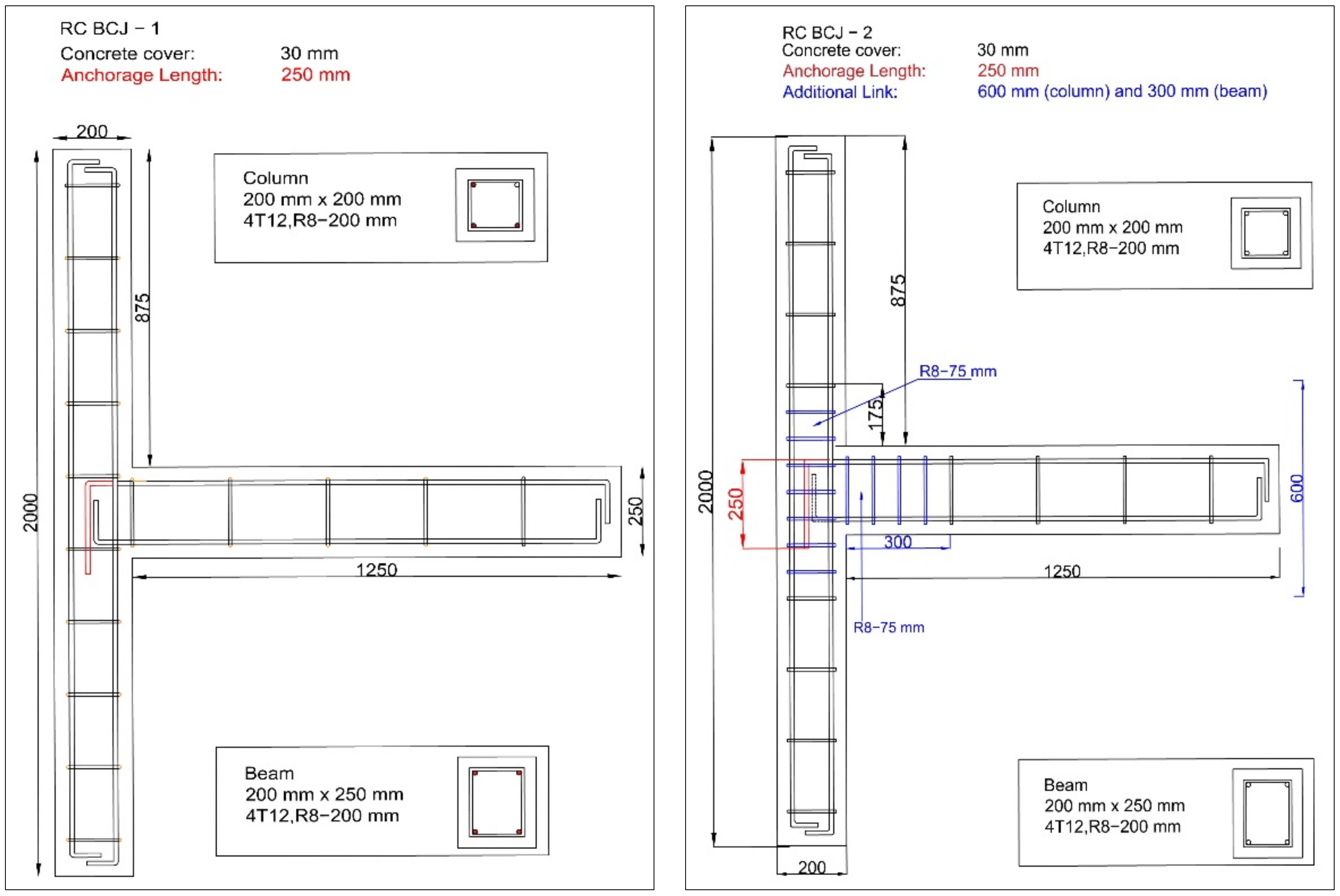
Figure 1. Detailing of every RC beam-column joint specimen.
Applsci 11 07700 g001aApplsci 11 07700 g001bApplsci 11 07700 g001c
Figure 2. Typical setup of RC beam-column joint specimen.
Applsci 11 07700 g002
Figure 3. Lateral cyclic loading history for RC beam-column joint specimen.
Applsci 11 07700 g003
Figure 4. Load−drift hysteretic relationships of test specimens.
Applsci 11 07700 g004aApplsci 11 07700 g004b
Figure 5. Crack patterns and damage of respective specimens.
Applsci 11 07700 g005
Figure 6. The basic ANN layer with interconnected nodes (reproduced from [73]).
Applsci 11 07700 g006
Figure 7. The framework of DL model (reproduced from [74]).
Applsci 11 07700 g007
Figure 8. The SVM framework (Dot products in kernel function).
Applsci 11 07700 g008
Figure 9. The framework model applied for all four prediction models from Rapidminer machine learning.
Applsci 11 07700 g009
Figure 10. The distribution of predicted crack width for (a) DL Max-out prediction model (b) DL Rectifier prediction model (c) SVM—dot prediction model and (d) SVM—neural prediction model.
Applsci 11 07700 g010aApplsci 11 07700 g010b
Figure 11. The distribution of predicted results according to every split ratio (a) 70:30, (b) 75:25, and (c) 80:20.
Applsci 11 07700 g011
Figure 12. The distribution of predicted results are dependent on inputs vector: (a) Seven inputs vector, (b) nine inputs vector, and (c) eleven inputs vector.
Applsci 11 07700 g012
Figure 13. The distribution of predicted crack width for: (a) Absolute error (AE), (b) prediction average (AE), and (c) root mean square error (RMSE).
Applsci 11 07700 g013
Table 1. The designed detailing of specimens.
SpecimenDetailingRemarks
ColumnBeamAt Joint
Main BarAdd. Shear Link Spacing (mm)Main BarAdd. Shear Link Spacing (mm)Anchorage Length
(mm)
BCJ-14T12-4T12-250Design based on British
Standard [33,34]
BCJ-24T12R8-75
(600 *)
4T12R8-75
(300)
250Strengthen at joint based on EC8 (Low to moderate seismic) [30]
BCJ-34T12R8-75
(850)
4T12R8-75
(600)
250Designed as in BCJ-2 with a 30% increased number of shear links
BCJ-44T12R8-50
(600)
4T12R8-50
(300)
250Designed as in BCJ-2 with minimum link spacing allowed in the seismic design
BCJ-54T12R8-754T12R8-75
(300)
180Designed as in BCJ-2 without anchorage length (U-bar)
BCJ-64T12R8-754T12R8-75
(300)
500Designed as in BCJ-2 with twice anchorage length
BCJ-74T12R8-754T12R8-75
(300)
750Designed as in BCJ-2 with thrice anchorage length
* Shear span of additional shear links.
Table 2. List of data opted as potential input parameters for modeling purposes.
NumParameters Obtained before and after Experimental TestingAbbrev.Unit
1.Reinforcement area Asmm2
2.Shear link spacing at beamSLBmm
3.Shear link spacing at columnSLCmm
4.Shear span for additional shear links at beamSSLBmm
5.Shear span for additional shear links at columnSSLCmm
6.Anchorage length at joint ALmm
7.Concrete compression strengthCcMPa
8.Concrete tensile strengthCtMPa
9.Tensile bar strengthTtMPa
10.Drift ratioDR%
11.Maximum positive load-carrying capacityQmax(+ve)kN
12.Maximum negative load-carrying capacityQmax(−ve)kN
Table 3. The details of four prediction models.
NoModelPrediction Method
1.Deep learning (DL)Max-out: Based on the maximum coordinate of the input vector.
2.Deep learning (DL)Rectifier: Rectifier Linear Unit (RLU), which chooses the maximum of (0, x) where x is the input value.
3.Support Vector
Machine (SVM)
Dot: The dot kernel is defined by k(x,y) = x × y, i.e., it is the inner product of x and y.
4.Support Vector
Machine (SVM)
Neural: The neural kernel is defined by a two-layered neural net tanh (ax × y + b), where a is alpha and b is the intercept constant.
These parameters can be adjusted using the kernel a and kernel b parameters. A common value for alpha is 1/N, where N is the data dimension.
Table 4. Inputs variable vector (7, 9, and 11 inputs).
List of Inputs7 Inputs Vector (X1–X7)9 Inputs Vector (Y1–Y9)11 Inputs Vector (Z1–Z11)
AsAsAs
OLB/COLB/COLB/C
SSLBSSLBSSLB
SSLCSSLCSSLC
ALALAL
CcCcCc
DRDRCt
Qmax(+ve)Tt
Qmax(−ve)DR
Qmax(+ve)
Qmax(-ve)
OutputCrack width (C.W.)
Table 5. Types of performance index (regression) used for SVM—dot model.
NoParameterDescription
1.Absolute error
(AE)
AE is determined by adding the variance of all expected values from the label attribute’s actual values and dividing the amount by the total number of predictions.
2.Prediction average (PA)PA is determined by adding all the real label values and dividing the total number of examples by this figure.
3.Root mean square error (RMSE)RMSE is a quadratic scoring method calculating the error’s average magnitude. It is the cumulative square root of variations between predictive and real observation.
Publisher’s Note: MDPI stays neutral with regard to jurisdictional claims in published maps and institutional affiliations.