Abstract
Dictionary learning has been an important role in the success of data representation. As a complete view of data representation, hybrid dictionary learning (HDL) is still in its infant stage. In previous HDL approaches, the scheme of how to learn an effective hybrid dictionary for image classification has not been well addressed. In this paper, we proposed a locality preserving and label-aware constraint-based hybrid dictionary learning (LPLC-HDL) method, and apply it in image classification effectively. More specifically, the locality information of the data is preserved by using a graph Laplacian matrix based on the shared dictionary for learning the commonality representation, and a label-aware constraint with group regularization is imposed on the coding coefficients corresponding to the class-specific dictionary for learning the particularity representation. Moreover, all the introduced constraints in the proposed LPLC-HDL method are based on the -norm regularization, which can be solved efficiently via employing an alternative optimization strategy. The extensive experiments on the benchmark image datasets demonstrate that our method is an improvement over previous competing methods on both the hand-crafted and deep features.
1. Introduction
Due to the insufficiency of data representation, Dictionary Learning (DL) has aroused considerable interest in the past decade and achieved much success in the various applications, such as image denoising [1,2], person re-identification [3,4] and vision recognition [5,6,7,8]. Generally speaking, the DL methods are developed based on a basic hypothesis, which are that a test signal can be well approximated using the linear combination of some atoms in a dictionary. Thus the dictionary usually plays an important role in the success of these applications. Traditionally, the DL methods can be roughly divided into two categories: The unsupervised DL methods and the supervised DL methods [9,10].
In the unsupervised DL methods, a dictionary is optimized to reconstruct all the training samples without any label assignment; hence, there is no class information in the learned dictionary. By further integrating the label information into dictionary learning, the supervised DL methods can achieve better classification performance than the unsupervised ones for image classification. Supervised dictionary learning encodes the input signals using the learned dictionary, then utilizes the representation coefficients or the residuals for classification. Thus the discriminative ability of the dictionary and the representative ability of the coding coefficients play the key roles in this kind of approach. According to the types of the dictionary, the supervised DL methods can be further divided into three categories: The class-shared DL methods, the class-specific DL methods and the hybrid DL methods [11].
The class-shared DL methods generally force the coding coefficients to be discriminative via learning a single dictionary shared by all the classes. Based on the K-SVD algorithm, Zhang and Li [5] proposed the Discriminative K-SVD (D-KSVD) method to construct a classification error term for learning a linear classifier. Jiang et al. [6] further proposed the Label Consistent K-SVD (LC-KSVD) which encourages the coding coefficients from the same class to be as similar as possible. Considering the characteristics of atoms, Song et al. [12] designed an indicator function to regularize the class-shared dictionary to improve the discriminative ability of coding coefficients. In general, the computation of the test stage is very efficient in the class-shared DL methods, but it is hard to improve the coefficients’ discriminativity for better classification performance as the class-shared dictionary is not enough for fitting the complex data.
In the class-specific dictionary learning, each sub-dictionary is assigned to a single class and the sub-dictionaries with the different classes are encouraged to be as independent as possible. As a representative class-specific DL method, Fisher Discrimination Dictionary Learning (FDDL) [13] employs Fisher discrimination criterion on the coding coefficients, then utilizes the representation residual of each class to establish the discriminative term. Using with the incoherence constraint, Ramirez et al. [14] proposed a structured dictionary learning scheme to promote the discriminative ability of the class-specific sub-dictionaries. Akhtar et al. [15] developed a Joint discriminative Bayesian Dictionary and Classifier learning (JBDC) model to associate the dictionary atoms by the class labels with Bernoulli distributions. The class-specific DL methods usually associate a dictionary atom to a single class directly; hence, the reconstruction error with respect to each class can be used for classification. However, the test stage of this category often requires the coefficient computation of test data over many sub-dictionaries.
In the hybrid dictionary learning, a dictionary is designed to have a set of class-shared atoms in addition to the class-specific sub-dictionaries. Wang and Kong [16] proposed a hybrid dictionary dubbed DL-COPAR to explicitly separate the common and particular features of the data, which also encourages the class-specific sub-dictionaries to be incoherent. Vu et al. [17] developed a Low-Rank Shared Dictionary Learning (LRSDL) method to preserve the common features of samples. Gao et al. [18] developed a Category-specific and Shared Dictionary Learning (CSDL) approach for fine-grained image classification. Wang et al. [19] designed a structured dictionary consisting of label-particular atoms corresponding to some class and shared atoms commonly used by all the classes, and introduced a Cross-Label Suppression for Dictionary Learning (CLSDL) to generate approximate sparse coding vectors for classification. To some extent, the hybrid dictionary is very effective at preserving the complex structure of the visual data. However, it is nontrivial to design the class-specific and shared dictionaries with the proper number of atoms, which often has a severe effect on classification performance.
In addition to utilizing the class label information, more and more supervised DL approaches have been proposed to incorporate the locality information of the data into the learned dictionary. By calculating the distances between the bases (atoms) and the training samples, Wang et al. [20] developed a Locality-constrained Linear Coding (LLC) model to select the k-nearest neighbor bases for coding, and set the coding coefficients of other atoms to zero. Wei et al. [21] proposed locality-sensitive dictionary learning to enhance the power of discrimination for sparse coding. Song et al. [22] integrated the locality constraints into the multi-layer discriminative dictionary to avoid the appearance of over-fitting. By coupling the locality reconstruction and the label reconstruction, the LCLE-DL method [7] ensures that the locality-based and label-based coding coefficients are as approximate to each other as possible. It is noted that the locality constraint in LCLE-DL may cause the dictionary atoms from the different classes to be similar, which weakens the discriminative ability of the learned dictionary.
It is observed that the real-world object categories are not only a marked difference, but are also strongly correlated in terms of the visual property, e.g., faces from the different persons often share similar illumination and pose variants; objects in the Caltech 101 dataset [23] have the correlated background. These correlations are not very helpful to distinguish the different categories, but without them the data with common features cannot be well represented. Thus, the dictionary learning approach should learn the distinctive features with the class-specific dictionary, and simultaneously exploit the common features of the correlated classes by learning a commonality dictionary. To this end, we proposed the locality preserving and label-aware constraint-based hybrid dictionary learning (LPLC-HDL) method for image classification, which is composed of a label-aware constraint, a group regularization and a locality constraint. The main contributions are summarized as follows.
- [1].
- The proposed LPLC-HDL method learns the hybrid dictionary by fully exploiting the locality information and the label information of the data. In this way, the learned hybrid dictionary can not only preserve the complex structural information of the data, but also have strong discriminativity for image classification.
- [2].
- In LPLC-HDL, a locality constraint is constructed to encourage the samples from different classes with similar features to have similar commonality representation; then, a label-aware constraint is integrated to make the class-specific dictionary sparsely represent the samples from the same class, so that the robust particularity–commonality representation can be obtained by the proposed LPLC-HDL.
- [3].
- In a departure from the competing methods which impose the -norm or -norm on the coefficients, LPLC-HDL consists of -norm constraints that can be calculated efficiently. The objective function is solved elegantly by employing an alternative optimization technique.
The rest of this paper is outlined as follows. Section 2 reviews the related work on our LPLC-HDL method. Then Section 3 presents the details of LPLC-HDL and an effective optimization is introduced in Section 4. To verify the efficiency of our method for image classification, the experiments are conducted in Section 5. Finally, the conclusion is summarized in Section 6.
2. Notation and Background
In this section, we first provide the notation used in this paper, then review the LCLE-DL algorithm and the objective function of hybrid dictionary learning (DL), which can be taken as the theoretical background of our LPLC-HDL method.
2.1. Notation
Let be a set of N training samples in an m dimension with class labels ; here, C is the class number of the training samples and is a matrix consisting of training samples of the ith class. Suppose and make up the learned hybrid dictionary from the training samples X, where is the atom number of shared dictionary, denotes the atom number of class-specific dictionary and is the atom number of ith class sub-dictionary. Let be the coding coefficients of training samples X over the hybrid dictionary D; then, and represent the coding coefficients over the shared dictionary and the ith class sub-dictionary, respectively.
According to [24], a row vector of coefficient matrix Z can be defined as a profile of the corresponding dictionary atom. Therefore, we can define a vector as the profile of atom for all the training samples, where the sub-vector is the sub-profile for the training samples of the cth class.
2.2. The LCLE-DL Algorithm
To improve the classification performance, the LCLE-DL algorithm [7] takes both the locality and label information of dictionary atoms into account in the learning process. This algorithm firstly constructs the locality constraint to ensure that similar profiles have similar atoms, then establishes the label embedding constraint to encourage the atoms of the same class to have similar profiles. The objective function of LCLE-DL is defined as follows.
where and denote the locality-based and the label-based coding coefficients, is the graph Laplacian matrix that is constructed by the atom’s similarity in the dictionary , is the scaled label matrix which is constructed using the label matrix of the dictionary . combined with the second term encodes the reconstruction under the locality constraint; combined with fourth term encodes the reconstruction under the label embedding; is used to transfer the label constraint to the locality constraint. and are the regularization parameters; the constraint on the atoms can avoid the scaling issue.
The LCLE-DL algorithm first exploits the K-SVD algorithm to learn sub-dictionaries using with the training samples . Similar to the label matrix of the training samples Y, the label matrix of the dictionary can be obtained as . Then a weighted label matrix is constructed by . Next, the label embedding of atoms is defined as
where is the scaled label matrix of the dictionary ; the above terms make the coding coefficients have a block-diagonal structure with strong discriminative information.
The learned dictionary inherits the manifold structure of the data via using the derived-graph Laplacian matrix L, and the optimal representation of the samples can be obtained with the label embedding of dictionary atoms. By combining the double reconstructions, LCLE-DL ensures the label-based and the locality-based coding coefficients are as approximate to each other as possible. However, the locality constraint is imposed on the class-specific dictionary in the LCLE-DL algorithm, which may cause the dictionary atoms from the different classes to be similar, thus the discriminative ability of the dictionary is weakened.
2.3. The Objective Function of Hybrid DL
In recent years, the hybrid DL [16,19,25,26] has been getting more and more attention in the classification problem. The hybrid dictionary has been shown to perform better than the other types of dictionaries, as it can preserve both the class-specific and common information of the data. To learn such a dictionary, we can define the objective function of Hybrid DL as follows.
where , is the dictionary shared by all the classes, is the ith class sub-dictionary, and are the coding coefficients of the samples from the ith class over and , and and denote the functions about the hybrid dictionary and the coding coefficients, respectively. The constraint of typically adopts [26] norm or [25,27] norm for sparse coding.
3. The Proposed Method
By learning the shared dictionary , the previous hybrid DL algorithms can capture the common features of the data, but they do not concern the correlation among these features, which will reduce the robustness of the learned dictionary. In this section, we firstly utilize the locality information of the atoms in to construct a locality constraint, then impose it on the coefficients , so that the correlation of the common features is captured explicitly and the learned dictionary is very robust concerning commonality representation. Moreover, once the correlation is discarded, the classification of a query sample will be dominated by the class-specific sub-dictionary corresponding to the correct class to reach minimized data fidelity.
To obtain the discriminative ability of the class-specific dictionary, we further introduce a label-aware constraint as well as group regularization on the distinctive coding coefficients for the particularity representation. Since this constraint integrated with the locality constraint to reconstruct the input data, they will reinforce each other in the learning process, which results in a discriminative hybrid dictionary for image classification.
Accordingly, the objective function of the proposed LPLC-HDL method can be formulated as follows.
where , and are the regularization parameters, which can adjust the weights of the label-aware constraint, the group regularization and the the locality constraint, respectively. Here we set the Euclidean length of all the atoms in the shared dictionary and the class-specific dictionary to be 1, which can avoid the scaling issue.
3.1. The Locality Constraint for Commonality Representation
Locality information of the data has played an important role in many real applications. By incorporating locality information for learning a dictionary, we can ensure that the samples with common features tend to have similar coding coefficients [7]. Further more, the dictionary atoms measure the similarity of the samples, which are more robust to the noise and outliers than the original samples. Hence, we use the atoms of the shared dictionary to capture the correlation among the common features and construct a locality constraint.
Based on the shared dictionary , we can construct a nearest neighbor graph as follows.
where is a parameter to control the exponential function, kNN() denotes k nearest neighbors of atom , indicates the similarity between the atoms and . For convenience of calculation, we invariably set the parameters and , as they have the stable values in the experiments.
Once is calculated, we construct a graph Laplacian matrix as follows.
Since is constructed based on the dictionary , it will be updated in coordination with in the learning process.
By now, we can obtain a locality constraint term for choosing graph Laplacian matrix as follows.
Because the profile and the atom have a one-to-one correspondence, the above equation ensures that similar atoms encourage similar profiles [7]. Hence, the correlated information of the common features can be inherited by the coefficient matrix and the graph Laplacian matrix .
3.2. The Constraints for Particularity Representation
3.2.1. The Label-Aware Constraint
To obtain the particularity representation for the classification, we will assign the labels to the atoms of the class-specific dictionary, as presented in [7,19]. If an atom , the label i will be assigned to the atom and kept invariant in the iterations. We take as the index set for the atoms of ith class sub-dictionary , and as the index set for all the atoms of the class-specific dictionary. For the particularity representation of samples , it is desirable that the large coefficients should mainly occur on the atoms in . In other words, the sub-profiles associated with the atoms in need to be suppressed to some extent.
For the ith class samples, we construct a matrix to pick up the sub-profiles from the representation , which locate at the atoms in rather than the atoms in , so that we can define a label-aware constraint term as follows.
and the matrix can be written as
where is the th entry of matrix . For the particularity representation , minimizing the label-aware constraint can suppress the large values in the sub-profiles associated with the atoms in , as well as encourage the large ones in the sub-profiles associated with ith class atoms. Therefore, it is expected that this constraint with a proper scalar can make the particularity representation approximately sparse. Besides, once a series of matrices are constructed, they will be unchanged in the iterations. Thus it is very efficient for coding over the class-specific dictionary.
3.2.2. The Group Regularization
Furthermore, to promote the consistency of particularity representation from the same class, we introduce the group regularization on . In light of the label information of training samples, assume one sample is related to one vertex; the vertices corresponding to the same class samples are connected and neighboring each other; thus, each class forms a densely connected sub-graph. Considering the training samples and their coding coefficients , we first define graph maps with mapping each graph to a line that consists of points, as follows
Here is the kth component of , which corresponds to the kth atom in the ith class sub-dictionary .
Then, we can calculate the variation for these graph maps as follows.
where denotes the normalized Laplacian of the overall graph for the ith class, which can be derived as
For the different classes, the vertices related to their samples should not be connected; thus, the graphs of C classes are isolated from each other. Therefore, we can obtain the total variation for graph maps of all the C classes as , where . Keeping this group regularization small will promote the consistency of the representation for the same class samples. Moreover, by combing it with the label-aware constraint, the coding coefficients for the different classes will be remarkably distinct with the large coefficients locating in the different areas, which is very favorable for the classification task.
4. Optimization Strategy and Classification
4.1. Optimization Strategy of LPLC-HDL
As the objective function in Equation (4) is not a jointly convex optimization problem for the variables (), it will be divided into two sub-problems by learning the shared and class-specific dictionaries alternatively, that is, updating variables () by fixing (), then updating variables () by fixing ().
We firstly use k-means algorithm to initialize shared dictionary by using all the training samples, then initialize ith class sub-dictionary by using the training samples and concatenate all these sub-dictionaries as the class-specific dictionary . Next, we compute the initialized coefficients and with the Multi-Variate Ridge Regression (MVRR) algorithm, and obtain the initialized matrix by Equation (6). In line with the corresponding sub-dictionaries, the serial of matrices and are constructed with Equations (9) and (12), respectively. After finishing the initialization, we can optimize the objective function as the following steps.
4.1.1. Shared Dictionary Learning
By fixing the variables (), the objective function of our LPLC-HDL for learning the shared dictionary becomes
where . To update the variables (), we turn to an iterative scheme, i.e., updating by fixing ), constructing based on ; updating by fixing . The detailed steps are elaborated as below.
(a) Update the shared dictionary and matrix
Without loss of generality, we first concentrate on optimizing the shared dictionary by fixing the variables (). The function (13) for becomes
where and . The quadratic constraint is introduced on each atom in to avoid the scaling issue risk. The above minimization can be solved by adopting the Lagrange dual algorithm presented as in [28].
(b) Update the commonality representation
By fixing the variables , the optimization of the commonality representation in Equation (13) can be formulated as
where and ; there is a closed-form solution for as all the above terms are based on the norm regularization.
By setting the derivative of (15) to zero, the optimal representation can be obtained as , where is an identity matrix.
4.1.2. Class-Specific Dictionary Learning
Assuming the variables () are fixed, the objective function (4) for learning the class-specific dictionary can be formulated as follows.
where . To update the variables (), we follow the iterative scheme presented in Section 4.1.1, i.e., updating by fixing ; then updating by fixing . The updating steps are elaborated as below.
(c) Update the class-specific dictionary
By fixing the variable , the optimization of dictionary can be simplified as the optimization of each atom . Provided and the other atoms in are fixed, to update the atom we can solve the optimization problem as follows.
where , and denotes the tth row vector of coefficient matrix . By introducing a variable , the solution of atom can be easily derived as
Consider the energy of each atom as being constrained in (16), the solution can be further normalized as
Because the atoms with indices out of are fixed when updating the atoms with indices in , we can compute in advance and take it into the calculation of to accelerate the update. Likewise, we successively update the atoms corresponding to with and obtain the overall class-specific dictionary .
(d) Update the particularity representation
For the particularity representation of the ith class , the optimization problem depending on it becomes
The solution of the above equation can be obtained by computing each code in as follows
where is the nth training sample of the ith class, is the code of and denotes the th entry of matrix . Since all the terms in Equation (21) are based on the quadratic form, the solution of can be easily obtained by setting its derivation to zero.
By using (12) and denoting as with the identity matrix , we can further obtain a matrix version for update as:
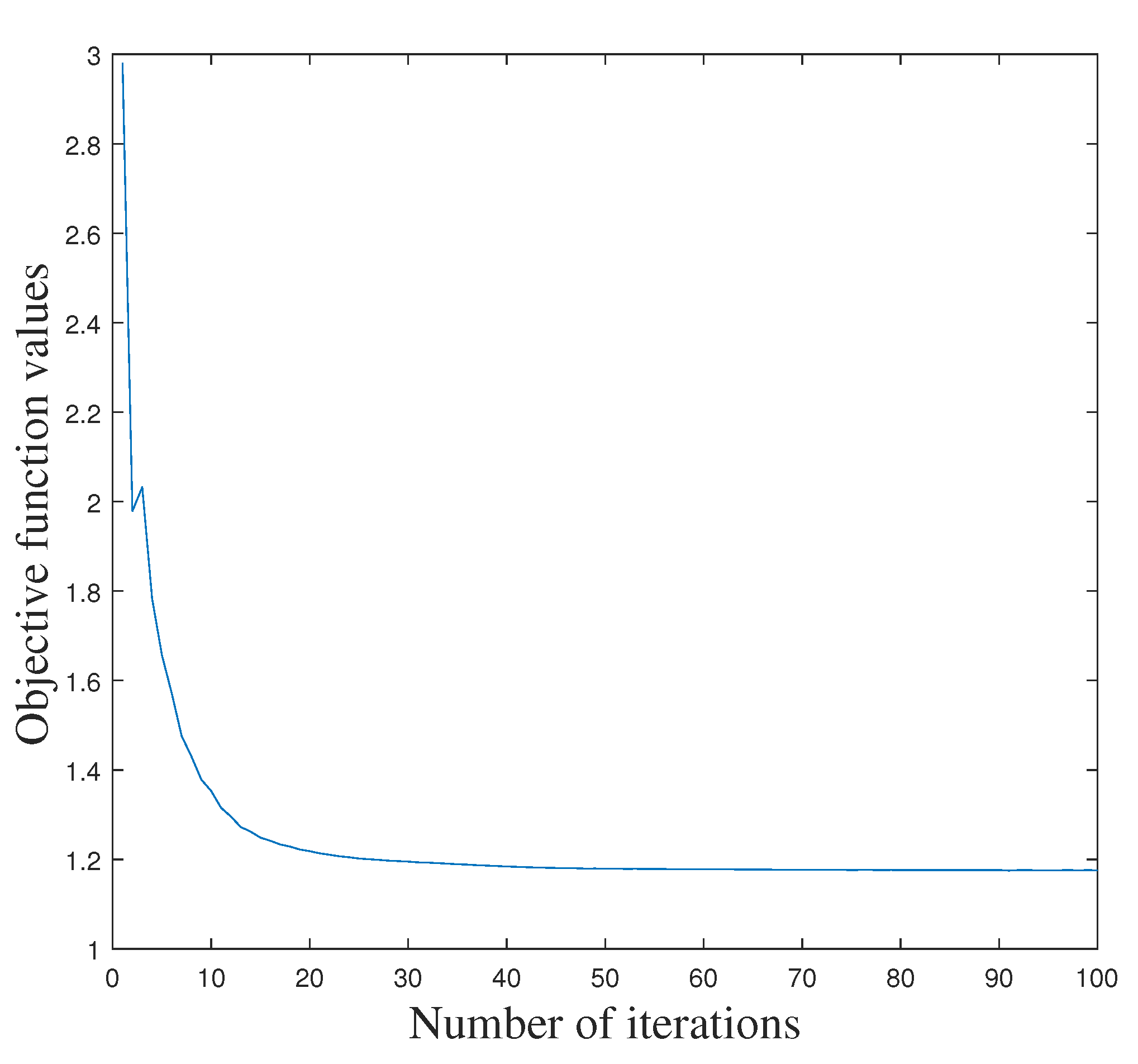
By repeating the steps (a)–(d), we can iteratively obtain all the optimal variables . The overall optimization of our LPLC-HDL is summarized in Algorithm 1. Moreover, the objective function value of Equation (4) decreases as the number of iterations increases on a given dataset. For example, the convergence curve of LPLC-HDL on the Yale face dataset [29] is illustrated in Figure 1. From it we can see that the proposed algorithm converges quickly, no more than 20 iterations.
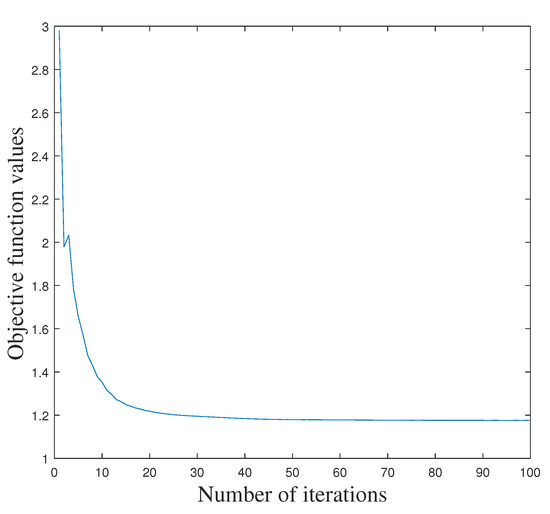
Figure 1.
The convergence curve of the proposed LPLC-HDL with the number of iterations on the Yale face dataset.
In Algorithm 1, the time complexity of our LPLC-HDL mainly comes from these parts: for updating the shared dictionary , for updating the graph Laplacian matrix , for updating the commonality representation , for updating the class-specific dictionary and for updating the particularity representation . Thus the final time complexity is in each iteration.
| Algorithm 1 Optimization procedure of the proposed LPLC-HDL |
|
4.2. Classification Procedure
After completing Algorithm 1, we can use the learned hybrid dictionary to represent a test sample and predict its label. Firstly, we find the commonality–particularity representation of a test sample by solving the following equation:
Secondly, we compute based on to exclude the contribution of the shared dictionary. Thus, the class label of can be determined by:
5. Experiments
In this section, we compare LPLC-HDL with the representative dictionary learning methods including D-KSVD [5], LC-KSVD [6], LCLE-DL [7], FDDL [13], DL-COPAR [16] and CLSDDL [19] on the Yale face dataset [29], the Extended YaleB face dataset [30], the Labeled Faces in the Wild (LFW) dataset [31] for face recognition, the Caltech-101 object dataset [23] and the Oxford 102 Flowers dataset [32] for object classification and flower classification, respectively. Moreover, we further compare it with the Sparse Representation based Classification (SRC) [33], the Collaborative Representation based Classifier (CRC) [34], the Probabilistic CRC (ProCRC) [35], the Sparsity Augmented Collaborative Representation (SACR) [36] and some other state-of-the-art methods on the particular datasets.
In the proposed LPLC-HDL method, the three parameters and are selected by five-fold cross validation on the training set, and their optimal values on each dataset are shown in Table 1. In addition, the atom numbers of the shared dictionary and the class-specific dictionary for each dataset are elaborated as detailed in the following experiments.

Table 1.
The parameters of the proposed LPLC-HDL method on each dataset.
5.1. Experiments on the Yale Face Dataset
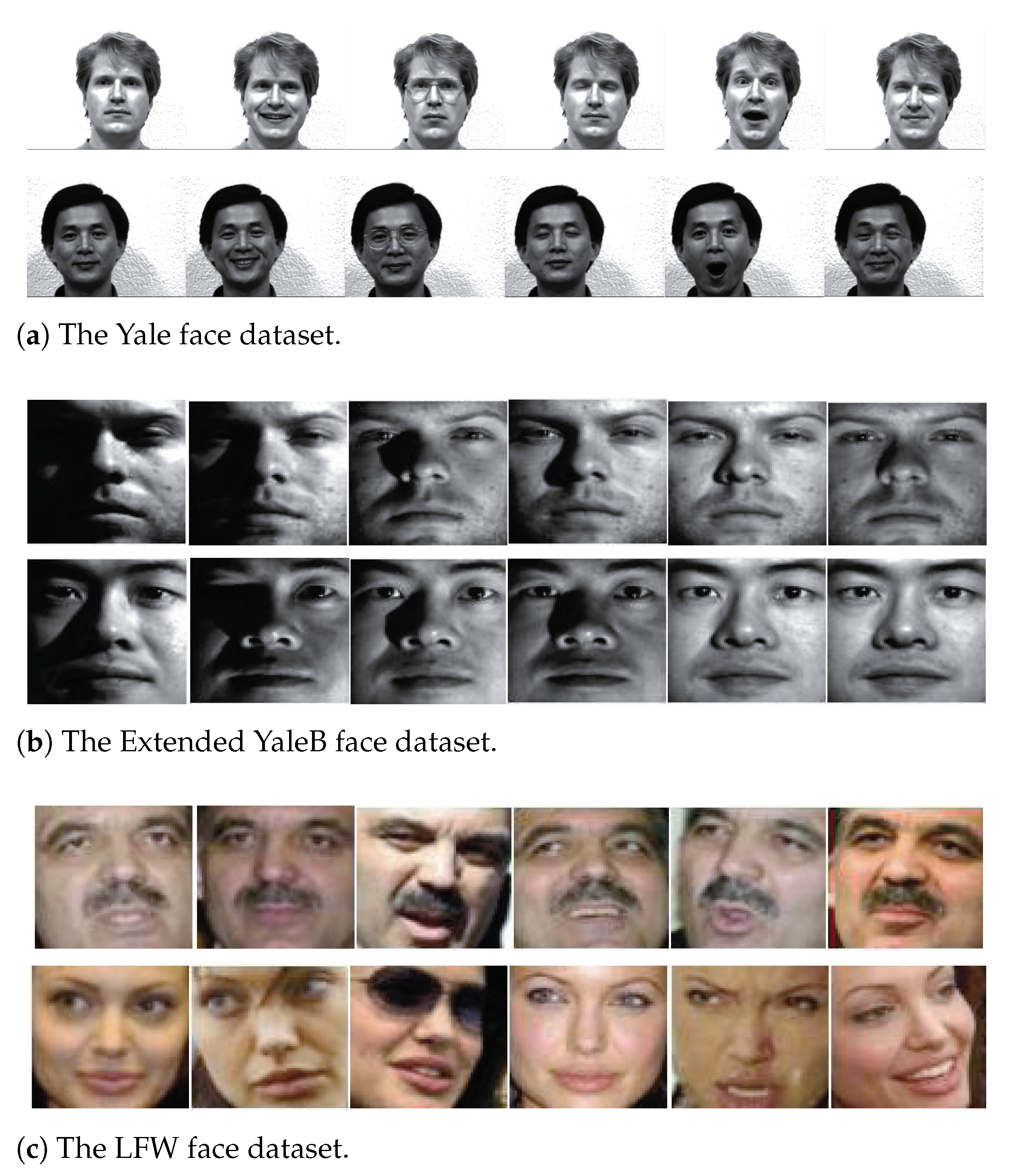
In the experiments, we first consider the Yale face dataset which contains 165 gray scale images for 15 individuals with 11 images per category. Each individual contains one different facial expression or configuration: Left-light, center-light, right-light, w/glasses, w/no glasses, happy, sad, normal, surprised, sleepy and wink, as shown in Figure 2a. Each image has pixel resolution, and is resized to 576-dimensional vectors with normalization for representation. Following the setting in [19], six images of each individual are randomly selected for training and the rest are used for testing. In addition, the number of dictionary atoms is set to + 60 = 120, which means four class-specific atoms for each individual and 60 shared atoms for all the individuals. The parameters of our LPLC-HDL on the Yale face dataset can be seen in Table 1.
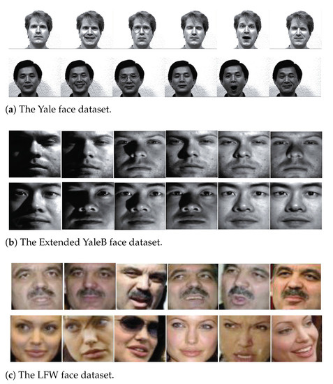
Figure 2.
The example images from the face datasets.
To acquire a stable recognition accuracy, we operate LPLC-HDL over 30 times rather than 10 times with independent training/testing splits. The comparison results on the Yale face dataset are listed in Table 2. Since the variations in terms of facial expression are complex, the variations in the testing samples cannot be well represented via directly using the training data. Hence SRC has worse accuracy than the other dictionary learning methods. We can also see that the hybrid dictionary learning methods including DL-COPAR [16], LRSDL [17] and CLSDDL [19] outperform the remaining competing approaches, and the proposed LPLC-HDL method achieves the best recognition accuracy of 97.01%, which illustrates that our method can distinguish the shared and class-specific information of face images more appropriately.

Table 2.
The recognition rates (%) on the Yale face dataset.
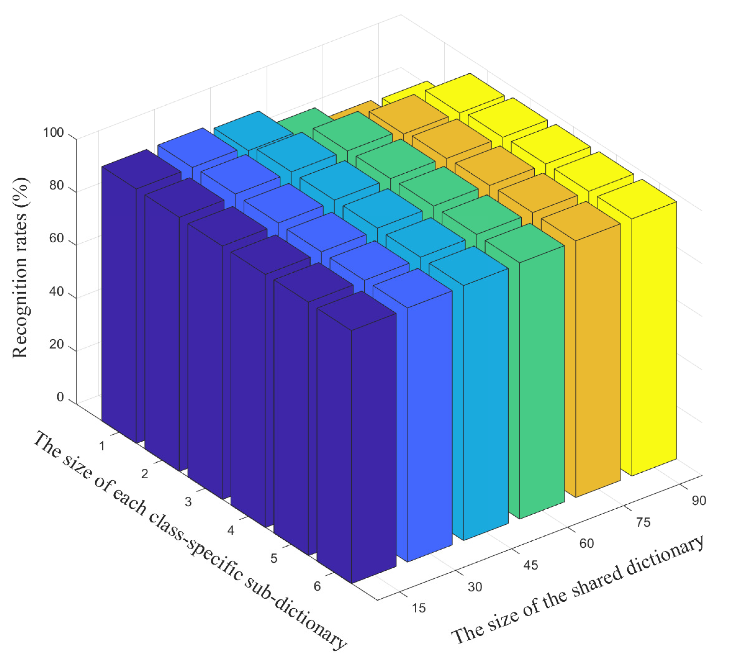
We further illustrate the performance of LPLC-HDL on face recognition accuracy with different sizes of the shared and class-specific dictionaries, as shown in Figure 3. From it we can see that a higher recognition accuracy on the Yale face dataset can be obtained by increasing the atom numbers of both the shared and class-specific dictionaries. Besides, Figure 3 also shows that when the number of the class-specific atoms is few, the recognition accuracy is sensitive to the number of the shared atoms, as the large shared dictionary is harmful to the discriminative power of the class-specific dictionary in this case. However, increasing the number of the class-specific atoms beyond the particular number of training samples of each class brings no notable increase in recognition accuracy. Considering that the large dictionary will slow down both the training time and the testing time, the atom numbers of the shared and class-specific dictionaries are not set to big values in the experiments.

Figure 3.
The recognition accuracy versus different sizes of the shared dictionary and the class-specific dictionary on the Yale face dataset.
5.2. Experiments on the Extended YaleB Face Dataset
The Extended YaleB face dataset contains 2414 frontal face images of 38 people. For each person, there are about 64 face images and the original images have pixels. This dataset is challenging due to varying poses and illumination conditions, as displayed in Figure 2b. For comparison, we use the normalized images instead of the original pixel information. In addition, we randomly select 20 images per category for training and take the rest as the testing images. The parameters of LPLC-HDL on the Extended YaleB face dataset are also shown in Table 1. The hybrid dictionary size is set to + 76 = 570, which denotes 13 class-specific atoms for each person and 76 shared atoms for all the persons, with the same structure adopted by the other hybrid dictionary learning methods.
We repeatedly run LPLC-HDL and all the comparison methods 10 times for reliable accuracy, and the average recognition rates are listed in Table 3. As shown in Table 3, compared with the K-SVD, D-KSVD, FDDL and LC-KSVD methods, LCLE-DL achieves a better recognition result with the same dictionary size. The reason for this behavior is that the LCLE-DL method can effectively utilize the locality and label information of the atoms in the dictionary learning. It is also shown that the hybrid dictionary learning methods, including DL-COPAR, LRSDL, CLSDDL and LPLC-HDL, generally outperform the other DL methods, which demonstrates the discriminative ability of the hybrid dictionary. By integrating the locality and label information into the hybrid dictionary, our LPLC-HDL method obtains the best recognition rate of 97.25%, which outperforms the second best approach CLSDDL-GC by 0.8%, and at least 1.2% higher than the other competing methods.

Table 3.
The recognition rates (%) on the Extended YaleB face dataset.
5.3. Experiments on the LFW Face Dataset
The LFW face dataset has more than 13,000 images with the name of the person pictured, and all of them are collected from the web for unconstrained face recognition and verification. Following the prior work [7], we use a subset of the LFW face dataset which consists of 1215 images from 86 persons. In this subset, there are around 11–20 images for each person, and all the images are resized to be . Some samples from this face dataset are shown in Figure 2c. For each person, eight samples are randomly selected for training and the remaining samples are taken for testing. The parameters of LPLC-HDL on the LFW face dataset are also shown in Table 1. In addition, the hybrid dictionary size is set to + 86 = 430, which means four class-specific atoms for each individual and 86 shared atoms for all the individuals.
We repeatedly run LPLC-HDL and the comparison methods 10 times, the average recognition rates are reported in Table 4, where the symbol ± denotes the standard deviation of average recognition rates. Similar to the results on the Extended YaleB face dataset, the LCLE-DL method achieves a higher recognition rate than the other shared or class-specific DL methods, and the hybrid dictionary learning methods, e.g., DL-COPAR, LRSDL, CLSDDL and LPLC-HDL, have a super performance in general. The proposed LPLC-HDL method obtains the best result with an average recognition rate of 42.39%, which is significantly better than all the comparison methods.

Table 4.
The recognition rates (%) on the LFW face dataset.
5.4. Object Classification
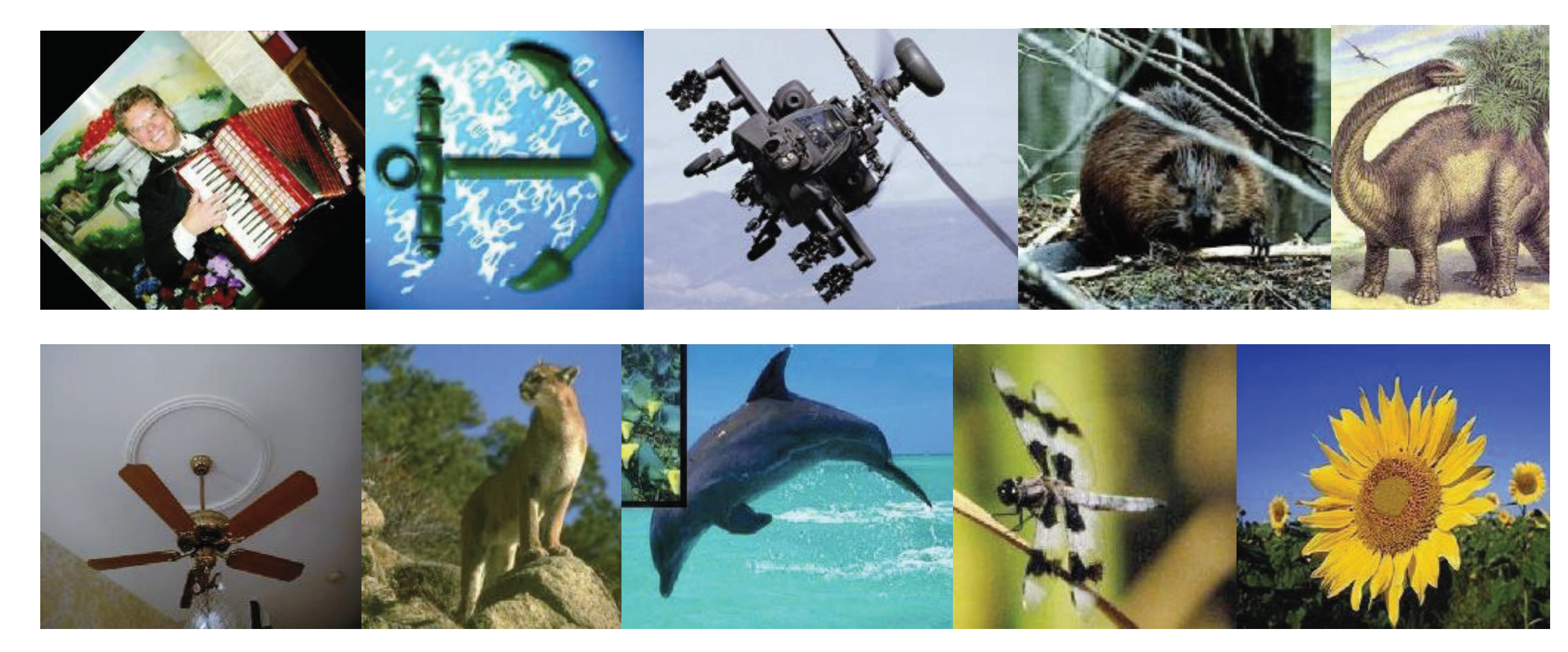
In this subsection, we evaluate LPLC-HDL on the Caltech-101 dataset [23] for object classification. This dataset contains a total of 9146 images from 101 object categories and a background category. The number of images for per category varies from a minimum of 31 to a maximum of 800 images. The resolution of each image is about , as shown in Figure 4. Following the settings [6,40], we perform the Spatial Pyramid Features (SPFs) on this dataset. Firstly, we partition each image into sub-regions with different spatial scales L = 0, 1, 2, then extract SIFT descriptors over a sub-region with a spacing of 8 pixels and concatenate them as the SPFs. Next, we encode the SPFs with a codebook of size 1024. Finally, the dimension of the features is reduced to 3000 using the the Principal Component Analysis (PCA) algorithm.
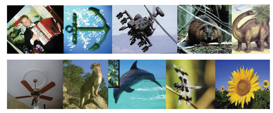
Figure 4.
Examples from the Caltech-101 object dataset.
For this dataset, 10 samples of each category are selected as the training data and the remaining are for testing. The parameters of LPLC-HDL on this dataset can be seen in Table 1. The hybrid dictionary size is set to + 100 = 1018, which denotes nine class-specific atoms for each category and 100 shared atoms for all the categories. The proposed LPLC-HDL and the comparison methods are carried out 10 times, the average classification rates are reported in Table 5. As can be seen in Table 5, our LPLC-HDL method achieves the best classification result again, with improvement margins of at least 1.3% compared with the comparison methods.

Table 5.
The classification results (%) on the Caltech101 object dataset.
5.5. Flower Classification
We finally evaluate the proposed LPLC-HDL on the Oxford 102 Flowers dataset [32] for fine-grained image classification, which consists of 8189 images from 102 categories, and each category contains at least 40 images. This dataset is very challenging because there exist large variations within the same category but small differences across several categories. The flowers appear at different scales, poses and lighting conditions; some flower images are shown in Figure 5. For each category, 10 images are used for training, 10 for validation, and the rest for testing, as in [32]. For ease of comparison, we take the convolutional neural network (CNN) features provided by Cai et al. [35] as the image-level features.
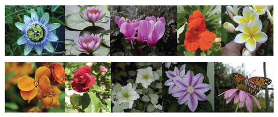
Figure 5.
Example images from the Oxford 102 Flowers dataset.
The parameters of LPLC-HDL on the Oxford 102 Flowers dataset can be seen in Table 1. The size of hybrid dictionary is set to be + 100 = 1018, which means nine atoms for each category and 100 atoms as the shared amount. We compare LPLC-HDL with different kinds of representative methods for flower classification, such as the basic classifiers (Softmax and linear SVM [38]), the recent ProCRC [35], the related DDL methods and the deep learning models. Following the common measurement [41,42], we evaluate the comparison methods by the average classification accuracy of all the categories, and the results are reported in Table 6. From it we can see that, taking the CNN features as the image-level features, the proposed LPLC-HDL method outperforms the basic classifiers and the competing DL methods. Compared with the other kinds of methods, LPLC-HDL is greatly superior to SparBases [43] and SMP [44]. Moreover, our method outperforms the recent deep learning models including GoogLeNet-GAP [45], ASPD [46] and AugHS [47], which need to design the special CNN architectures for flower classification.

Table 6.
The classification results (%) on the Oxford 102 Flowers dataset.
5.6. Parameter Sensitivity
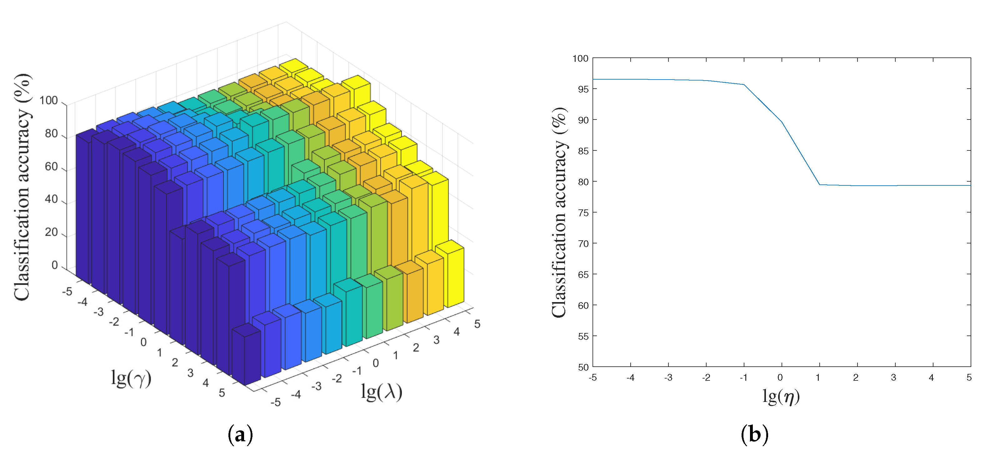
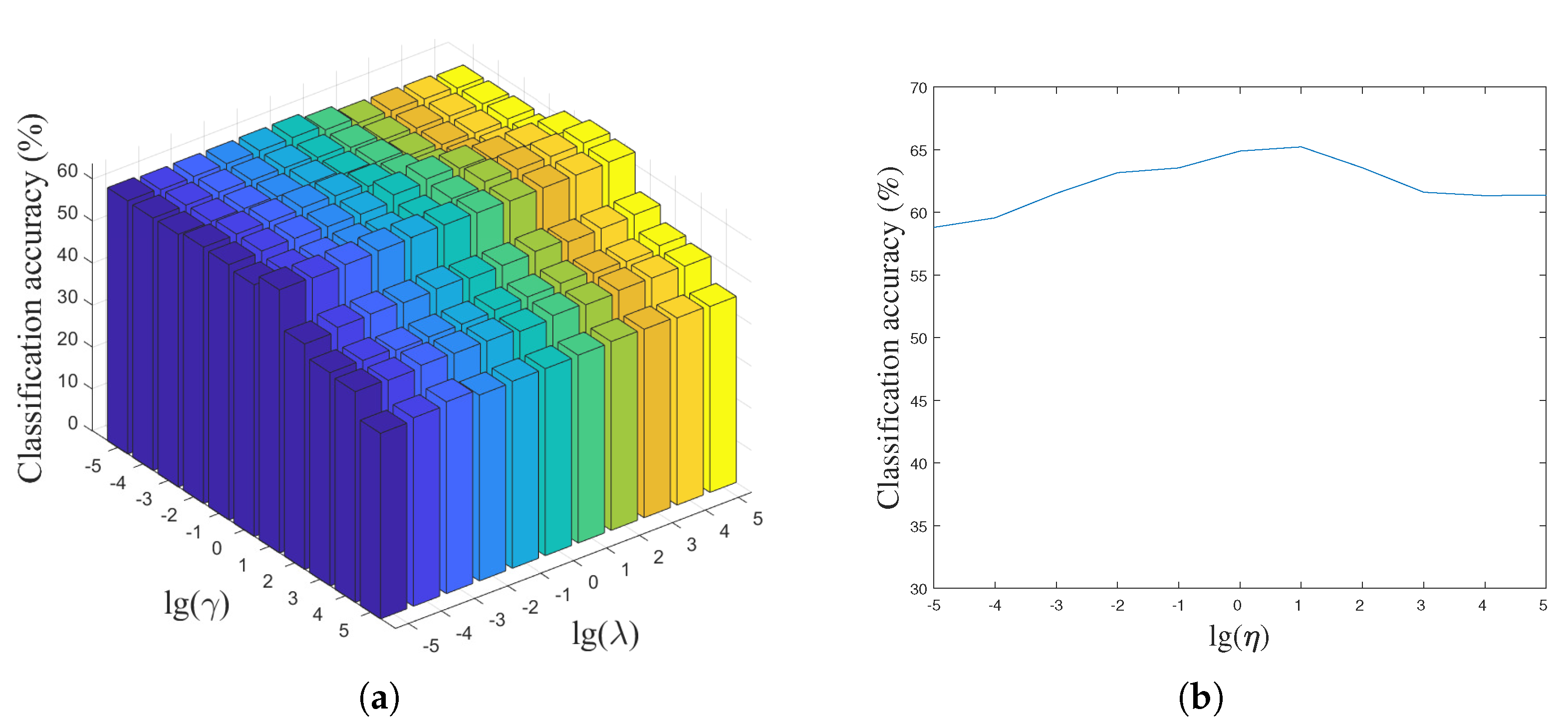
In the proposed LPLC-HDL method, there are three key parameters, i.e., , and , which are used to balance the importance of the label-aware constraint, the group regularization and the locality constraint. To analyze the sensitivity of the parameters, we define a candidate set , , , , , , , , , , for them and then perform LPLC-HDL with different combinations of the parameters on the Yale face dataset and the Caltech 101 dataset. By fixing the parameter , the classification accuracy versus different values of the parameters and are shown in Figure 6a and Figure 7a. As can be seen in the figures, the best classification result can be obtained when the parameters and locate in a feasible range. When is very small, the effect of the group regularization is limited, leading to weak discrimination of the class-specific dictionary. On the other hand, when becomes very large, the classification accuracy drops as the remaining terms in (4) become less important, which decreases the representation ability of the hybrid dictionary.
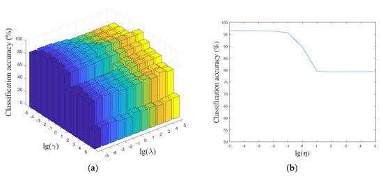
Figure 6.
The classification accuracy versus parameters , and on the Yale face dataset; (a) parameter is fixed; (b) parameters and are fixed.

Figure 7.
The classification accuracy versus parameters , and on the Caltech 101 object dataset; (a) parameter is fixed; (b) parameters and are fixed.
By fixing the parameters and , the classification accuracy versus different values of the parameter are shown in Figure 6b and Figure 7b. From them we can see that the classification accuracy is insensitive to the parameter when its value located in a certain range, e.g., on the Yale face dataset. It should be noted that the incoherence between the shared and class-specific dictionaries is increased with increasing parameter , which influences the reconstruction of the test data and decreases the classification accuracy.
Due to the diversity of the datasets, it is still an open problem to adaptively select the optimal parameters for the different datasets. In the experiments, we use an effective and simple way to find the optimal values for the parameters , and . Based on the previous analysis, we first fix the parameter to a small value such as 0.01, then search the candidate combination of the parameters and from the coarse set of , , , , , , , , , , . According to the best coarse combination of them, we can further define a fine candidate set where their optimal values may exist. Then we perform the proposed LPLC-HDL again with different combinations of the parameters and selected from the fine candidate set. This way, we can obtain the optimal values of the parameters for all the experimental datasets: hence, the best classification results are guaranteed.
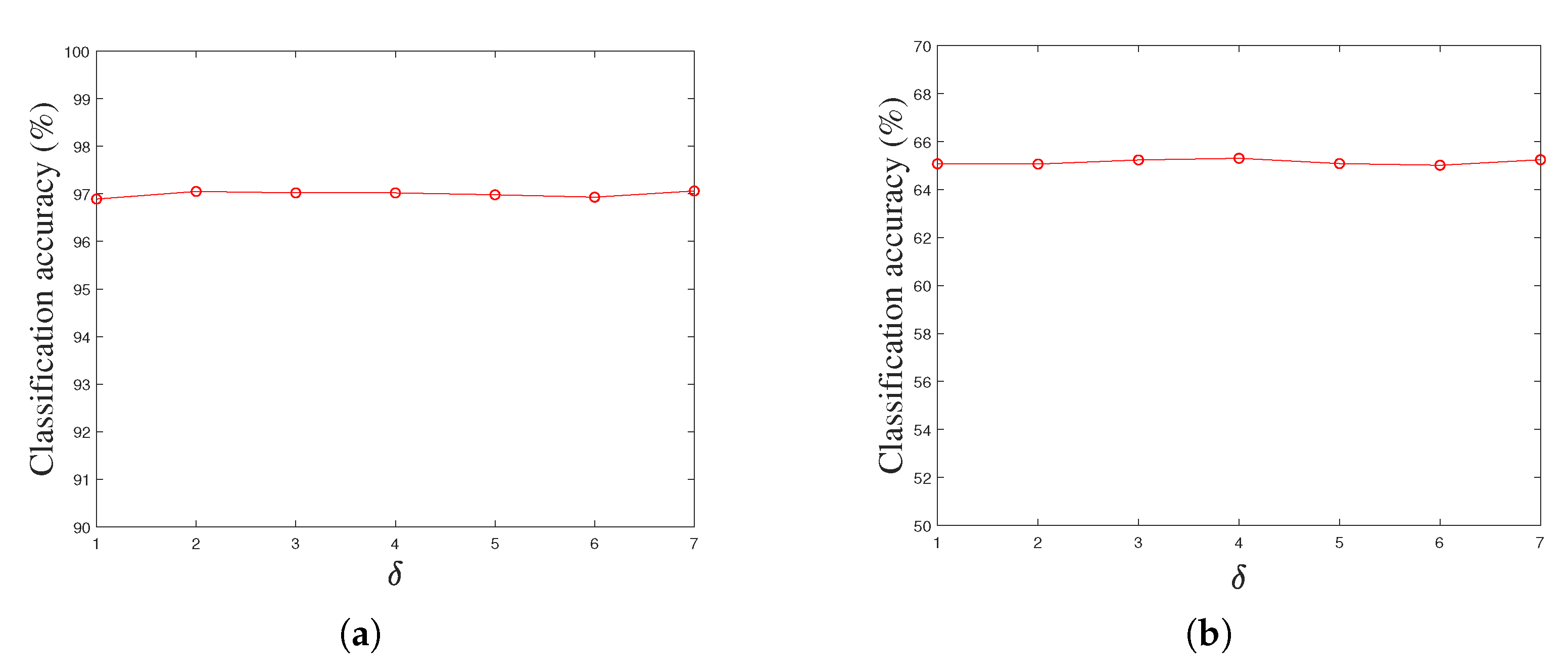
Besides the key parameters , and in our LPLC-HDL method, there are also the parameters and k in the proposed locality constraint. In the experiments, we find that these two parameters have stable values on the experimental datasets. For example, Figure 8a,b show the classification accuracies of our LPLC-HDL method with respect to the parameter by fixing the remaining parameters on the Yale face dataset and the Caltech 101 dataset. From the subfigures, we can see that the classification accuracy is insensitive to the parameter , and the approximate best result can be obtained when . For the parameter k, this similar phenomenon can be observed on the experimental datasets. Thus we can set and in our LPLC-HDL method for convenience of calculation.
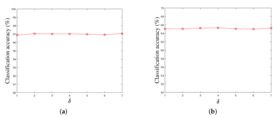
Figure 8.
The classification accuracy versus parameter on (a) the Yale face dataset, and (b) the Caltech 101 object dataset by fixing the parameters , , and k.
5.7. Evaluation of Computational Time
We also conducted experiments to evaluate the running time of the proposed LPLC-HDL and other representative DL methods on the two face datasets and the Caltech-101 dataset, the comparison results are listed in Table 7. “Train” denotes the running time of each iteration, and “Test” is the average processing time for classifying one test sample. All the experiments are conducted on a 64-bit computer with Intel i7-7700 3.6 GHz CPU and 12 GB RAM under the MATLAB R2019b programming environment. From Table 7, we can see that, although slower than CLSDDL-LC [19], the training efficiency of LPLC-HDL is obviously higher than that of D-KSVD [5], LC-KSVD [6], FDDL [13] and DL-COPAR [16]. In the testing stage, the proposed LPLC-HDL has similar testing efficiency as D-KSVD and LC-KSVD, and the testing process of LPLC-HDL is much faster than that of FDDL and DL-COPAR. Specifically, the average time for classifying a test image by LPLC-HDL is always less than that of CLSDDL-LC on the experiments.

Table 7.
The computational times (second) on the experimental datasets.
6. Conclusions
In this paper, we propose a novel hybrid dictionary learning (LPLC-HDL) method by taking advantage of the locality and label information of the data, which can solve the image classification task effectively. The LPLC-HDL method incorporates the locality constraint with the label-aware constraint to more appropriately distinguish the shared and particularity information. More specifically, the locality constraint on the shared dictionary is used to model the similar features of the images from different classes; the label-aware constraint and the group regularization are coupled to make the class-specific dictionary more discriminative. An effective alternative strategy is developed to solve the objective function of LPLC-HDL. After training the hybrid dictionary, the class label of the test image can be predicted more accurately by excluding the contribution of the shared dictionary. The experimental results on three face datasets, the object dataset and the flower dataset demonstrate that our method has effectiveness and superiority for image classification.
Author Contributions
Methodology, J.S. and Z.L.; Software, L.W. and M.L.; Project administration, M.Z. and Q.W. All authors have read and agreed to the published version of the manuscript.
Funding
This work was supported in part by the National Natural Science Foundation of China (Nos. 62002102, 62176113), in part by the Leading talents of science and technology in the Central Plain of China under Grants no. 214200510012, the Key Technologies R & D Program of Henan Province (Nos. 212102210088, 202102210169), the Basic Research Projects in the University of Henan Province (No. 19zx010), Guizhou Provincial Science and Technology Foundation ([2020]1Y253), Henan Postdoctoral Foundation, in part by the Luoyang Major Scientific and Technological Innovation Projects under Grant No.2101017A, and Foundation from the Postdoctoral Research Station of Control Science and Engineering at Henan University of Science and Technology.
Institutional Review Board Statement
Not applicable.
Informed Consent Statement
Not applicable.
Data Availability Statement
Not applicable.
Conflicts of Interest
The authors declare no conflict of interest.
References
- Elad, M.; Aharon, M. Image denoising via sparse and redundant representations over learned dictionaries. IEEE Trans. Image Process. 2006, 15, 3736–3745. [Google Scholar] [CrossRef] [PubMed]
- Yan, R.; Shao, L.; Liu, Y. Nonlocal Hierarchical Dictionary Learning Using Wavelets for Image Denoising. IEEE Trans. Image Process. 2013, 22, 4689–4698. [Google Scholar] [CrossRef]
- Li, S.; Shao, M.; Fu, Y. Person Re-identification by Cross-View Multi-Level Dictionary Learning. IEEE Trans. Pattern Anal. Mach. Intell. 2018, 40, 2963–2977. [Google Scholar] [CrossRef]
- Li, K.; Ding, Z.; Li, S.; Fu, Y. Toward Resolution-Invariant Person Reidentification via Projective Dictionary Learning. IEEE Trans. Neural Netw. Learn. Syst. 2019, 30, 1896–1907. [Google Scholar] [CrossRef]
- Zhang, Q.; Li, B. Discriminative K-SVD for dictionary learning in face recognition. In Proceedings of the IEEE Conference on Computer Vision and Pattern Recognition, San Francisco, CA, USA, 13–18 June 2010; pp. 2691–2698. [Google Scholar]
- Jiang, Z.; Lin, Z.; Davis, L.S. Label Consistent K-SVD: Learning a Discriminative Dictionary for Recognition. IEEE Trans. Pattern Anal. Mach. Intell. 2013, 35, 2651–2664. [Google Scholar] [CrossRef]
- Li, Z.; Lai, Z.; Xu, Y.; Yang, J.; Zhang, D. A Locality-Constrained and Label Embedding Dictionary Learning Algorithm for Image Classification. IEEE Trans. Neural Netw. Learn. Syst. 2017, 28, 278–293. [Google Scholar] [CrossRef]
- Gu, S.; Zhang, L.; Zuo, W.; Feng, X. Projective dictionary pair learning for pattern classification. In Proceedings of the 27th International Conference on Neural Information Processing Systems, Montreal, QC, Canada, 8–13 December 2014; pp. 793–801. [Google Scholar]
- Mairal, J.; Ponce, J.; Sapiro, G.; Zisserman, A.; Bach, F.R. Supervised dictionary learning. In Proceedings of the 23th International Conference on Neural Information Processing Systems, Whistler, BC, Canada, 6–11 December 2009; pp. 1033–1040. [Google Scholar]
- Mairal, J.; Bach, F.; Ponce, J. Task-Driven Dictionary Learning. IEEE Trans. Pattern Anal. Mach. Intell. 2012, 34, 791–804. [Google Scholar] [CrossRef] [PubMed] [Green Version]
- Song, J.; Xie, X.; Shi, G.; Dong, W. Exploiting class-wise coding coefficients: Learning a discriminative dictionary for pattern classification. Neurocomputing 2018, 321, 114–125. [Google Scholar] [CrossRef]
- Song, Y.; Zhang, Z.; Liu, L.; Rahimpour, A.; Qi, H. Dictionary Reduction: Automatic Compact Dictionary Learning for Classification. In Proceedings of the Asian Conference on Computer Vision, Taipei, Taiwan, 21–23 November 2016; pp. 305–320. [Google Scholar]
- Yang, M.; Zhang, L.; Feng, X.; Zhang, D. Fisher Discrimination Dictionary Learning for sparse representation. In Proceedings of the International Conference on Computer Vision, Barcelona, Spain, 6–13 November 2011; pp. 543–550. [Google Scholar]
- Ramirez, I.; Sprechmann, P.; Sapiro, G. Classification and clustering via dictionary learning with structured incoherence and shared features. In Proceedings of the IEEE Conference on Computer Vision and Pattern Recognition, San Francisco, CA, USA, 13–18 June 2010; pp. 3501–3508. [Google Scholar]
- Akhtar, N.; Mian, A.; Porikli, F. Joint discriminative bayesian dictionary and classifier learning. In Proceedings of the IEEE Conference on Computer Vision and Pattern Recognition, Honolulu, HI, USA, 21–26 July 2017; pp. 3919–3928. [Google Scholar]
- Wang, D.; Kong, S. A classification-oriented dictionary learning model: Explicitly learning the particularity and commonality across categories. Pattern Recognit. 2014, 47, 885–898. [Google Scholar] [CrossRef]
- Vu, T.H.; Monga, V. Fast low-rank shared dictionary learning for image classification. IEEE Trans. Image Process. 2017, 26, 5160–5175. [Google Scholar] [CrossRef] [PubMed]
- Gao, S.; Tsang, I.H.; Ma, Y. Learning Category-Specific Dictionary and Shared Dictionary for Fine-Grained Image Categorization. IEEE Trans. Image Process. 2014, 23, 623–634. [Google Scholar] [PubMed]
- Wang, X.; Gu, Y. Cross-label Suppression: A Discriminative and Fast Dictionary Learning with Group Regularization. IEEE Trans. Image Process. 2017, 26, 3859–3873. [Google Scholar] [CrossRef] [PubMed] [Green Version]
- Wang, J.; Yang, J.; Kai, Y.; Lv, F.; Gong, Y. Locality-constrained Linear Coding for image classification. In Proceedings of the IEEE Conference on Computer Vision and Pattern Recognition, San Francisco, CA, USA, 13–18 June 2010; pp. 3360–3367. [Google Scholar]
- Wei, C.P.; Chao, Y.W.; Yeh, Y.R.; Wang, Y.C.F. Locality-sensitive dictionary learning for sparse representation based classification. Pattern Recognit. 2013, 46, 1277–1287. [Google Scholar] [CrossRef]
- Song, J.; Xie, X.; Shi, G.; Dong, W. Multi-layer Discriminative Dictionary Learning with Locality Constraint for Image Classification. Pattern Recognit. 2019, 91, 135–146. [Google Scholar] [CrossRef]
- Fei-Fei, L.; Fergus, R.; Perona, P. Learning Generative Visual Models from Few Training Examples: An Incremental Bayesian Approach Tested on 101 Object Categories. In Proceedings of the IEEE Conference on Computer Vision and Pattern Recognition, Washington, DC, USA, 27 June–2 July 2004; pp. 59–70. [Google Scholar]
- Sadeghi, M.; Babaie-Zadeh, M.; Jutten, C. Learning overcomplete dictionaries based on atom-by-atom updating. IEEE Trans. Signal Process. 2014, 62, 883–891. [Google Scholar] [CrossRef] [Green Version]
- Sun, Y.; Liu, Q.; Tang, J.; Tao, D. Learning Discriminative Dictionary for Group Sparse Representation. IEEE Trans. Image Process. 2014, 23, 3816–3828. [Google Scholar] [CrossRef]
- Wen, Z.; Hou, B.; Jiao, L. Discriminative Dictionary Learning with Two-Level Low Rank and Group Sparse Decomposition for Image Classification. IEEE Trans. Cybern. 2017, 47, 3758–3771. [Google Scholar] [CrossRef]
- Wang, C.P.; Wei, W.; Zhang, J.S.; Song, H.B. Robust face recognition via discriminative and common hybrid dictionary learning. Appl. Intell. 2017, 48, 156–165. [Google Scholar] [CrossRef]
- Boyd, S.; Parikh, N.; Chu, E.; Peleato, B.; Eckstein, J. Distributed Optimization and Statistical Learning via the Alternating Direction Method of Multipliers; Now Publishers Inc.: Delft, The Netherlands, 2011; Volume 3, pp. 1–122. [Google Scholar]
- Georghiades, A.S.; Belhumeur, P.N.; Kriegman, D.J. From few to many: Illumination cone models for face recognition under variable lighting and pose. IEEE Trans. Pattern Anal. Mach. Intell. 2001, 23, 643–660. [Google Scholar] [CrossRef] [Green Version]
- Lee, K.C.; Ho, J.; Kriegman, D.J. Acquiring linear subspaces for face recognition under variable lighting. IEEE Trans. Pattern Anal. Mach. Intell. 2005, 27, 684–698. [Google Scholar]
- Huang, G.B.; Ramesh, M.; Berg, T.; Learned-Miller, E. Labeled Faces in the Wild: A Database for Studying Face Recognition in Unconstrained Environments; Technical Report 07-49; University of Massachusetts: Amherst, MA, USA, 2007. [Google Scholar]
- Nilsback, M.E.; Zisserman, A. Automated Flower Classification over a Large Number of Classes. In Proceedings of the Sixth Indian Conference on Computer Vision, Graphics & Image Processing, Bhubaneswar, India, 16–19 December 2008; pp. 722–729. [Google Scholar]
- Wright, J.; Yang, A.Y.; Ganesh, A.; Sastry, S.S.; Ma, Y. Robust Face Recognition via Sparse Representation. IEEE Trans. Pattern Anal. Mach. Intell. 2009, 31, 210–227. [Google Scholar] [CrossRef] [PubMed] [Green Version]
- Zhang, L.; Yang, M.; Feng, X. Sparse representation or collaborative representation: Which helps face recognition? In Proceedings of the International Conference on Computer Vision, Barcelona, Spain, 6–13 November 2011; pp. 471–478. [Google Scholar]
- Cai, S.; Zhang, L.; Zuo, W.; Feng, X. A probabilistic collaborative representation based approach for pattern classification. In Proceedings of the IEEE Conference on Computer Vision and Pattern Recognition, Las Vegas, NV, USA, 26 June–1 July 2016; pp. 2950–2959. [Google Scholar]
- Akhtar, N.; Shafait, F.; Mian, A. Efficient classification with sparsity augmented collaborative representation. Pattern Recognit. 2017, 65, 136–145. [Google Scholar] [CrossRef]
- Yang, J.; Yu, K.; Gong, Y.; Huang, T. Linear spatial pyramid matching using sparse coding for image classification. In Proceedings of the IEEE Conference on Computer Vision and Pattern Recognition, Miami, FL, USA, 20–25 June 2009; pp. 1794–1801. [Google Scholar]
- Fan, R.E.; Chang, K.W.; Hsieh, C.J.; Wang, X.R.; Lin, C.J. LIBLINEAR: A library for large linear classification. J. Mach. Learn. Res. 2008, 9, 1871–1874. [Google Scholar]
- Aharon, M.; Elad, M.; Bruckstein, A. K-SVD: An Algorithm for Designing Overcomplete Dictionaries for Sparse Representation. IEEE Trans. Signal Process. 2006, 54, 4311–4322. [Google Scholar] [CrossRef]
- Lazebnik, S.; Schmid, C.; Ponce, J. Beyond bags of features: Spatial pyramid matching for recognizing natural scene categories. In Proceedings of the IEEE Conference on Computer Vision and Pattern Recognition, New York, NY, USA, 17–22 June 2006; pp. 2169–2178. [Google Scholar]
- Razavian, A.S.; Azizpour, H.; Sullivan, J.; Carlsson, S. CNN Features Off-the-Shelf: An Astounding Baseline for Recognition. In Proceedings of the IEEE Conference on Computer Vision and Pattern Recognition, Columbus, OH, USA, 23–28 June 2014; pp. 512–519. [Google Scholar]
- Azizpour, H.; Razavian, A.S.; Sullivan, J.; Maki, A.; Carlsson, S. From Generic to Specific Deep Representations for Visual Recognition. In Proceedings of the IEEE Conference on Computer Vision and Pattern Recognition, Boston, MA, USA, 7–12 June 2015; pp. 36–45. [Google Scholar]
- Yao, B.; Jiang, X.; Khosla, A.; Lin, A.L.; Guibas, L.; Fei-Fei, L. Human action recognition by learning bases of action attributes and parts. In Proceedings of the International Conference on Computer Vision, Barcelona, Spain, 6–13 November 2011; pp. 1331–1338. [Google Scholar]
- Khan, F.S.; van de Weijer, J.; Anwer, R.M.; Felsberg, M.; Gatta, C. Semantic pyramids for gender and action recognition. IEEE Trans. Image Process. 2014, 23, 3633–3645. [Google Scholar] [CrossRef] [Green Version]
- Zhou, B.; Khosla, A.; Lapedriza, A.; Oliva, A.; Torralba, A. Learning deep features for discriminative localization. In Proceedings of the IEEE Conference on Computer Vision and Pattern Recognition, Las Vegas, NV, USA, 26 June–1 July 2016; pp. 2921–2929. [Google Scholar]
- Khan, F.S.; Xu, J.; Van De Weijer, J.; Bagdanov, A.D.; Anwer, R.M.; Lopez, A.M. Recognizing actions through action-specific person detection. IEEE Trans. Image Process. 2015, 24, 4422–4432. [Google Scholar] [PubMed]
- Qi, T.; Xu, Y.; Quan, Y.; Wang, Y.; Ling, H. Image-based action recognition using hint-enhanced deep neural networks. Neurocomputing 2017, 267, 475–488. [Google Scholar] [CrossRef]
- Chien, J.-T.; Wu, C.-C. Discriminant waveletfaces and nearest feature classifiers for face recognition. IEEE Trans. Pattern Anal. Mach. Intell. 2002, 24, 1644–1649. [Google Scholar] [CrossRef]
- Simon, M.; Rodner, E. Neural Activation Constellations: Unsupervised Part Model Discovery with Convolutional Networks. In Proceedings of the International Conference on Computer Vision, Santiago, Chile, 7–13 December 2015; pp. 1143–1151. [Google Scholar]
- Angelova, A.; Zhu, S. Efficient Object Detection and Segmentation for Fine-Grained Recognition. In Proceedings of the IEEE Conference on Computer Vision and Pattern Recognition, Portland, OR, USA, 23–28 June 2013; pp. 811–818. [Google Scholar]
Publisher’s Note: MDPI stays neutral with regard to jurisdictional claims in published maps and institutional affiliations. |
© 2021 by the authors. Licensee MDPI, Basel, Switzerland. This article is an open access article distributed under the terms and conditions of the Creative Commons Attribution (CC BY) license (https://creativecommons.org/licenses/by/4.0/).

