4.1. Maximize the Sphere in the Useful Workspace of the 2PRU-1PRS
We know that the geometry parameters that affect the workspace are the radius of the mobile platform (R), the radius of the fixed platform (H) and the length of the limbs (L), while the radius of the limbs and the thickness of the mobile platform do not affect the workspace. Accordingly, we obtain the optimum H, L and R combination to obtain the useful workspace with the biggest sphere in it. The first step is to define a set of GP combinations that will be studied, the
StudyVariables. We define the ranges of the geometry parameters, shown in
Table 1.
We define the number of discretizations for each GP to be 10, so we obtain the 1000 GP possible combinations. Optimizing all of them would result in a very high computational cost, so we apply the restrictions that the geometry of the manipulator has to satisfy.
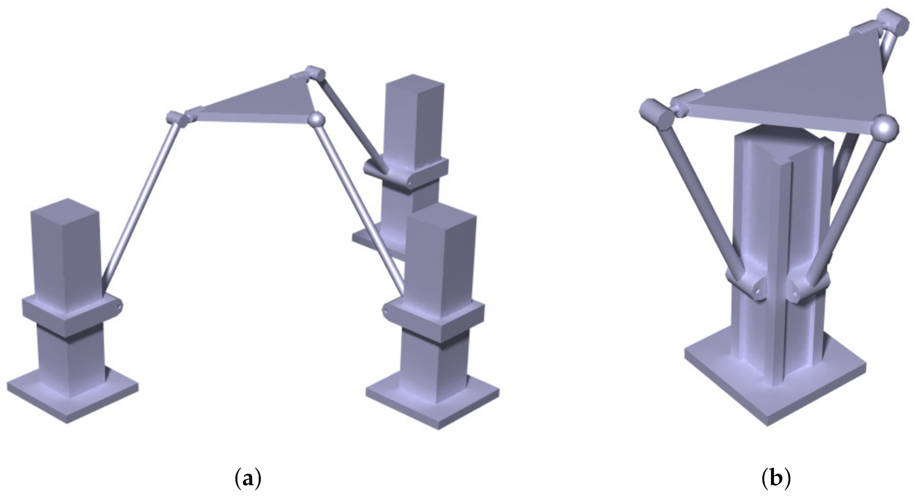
As we observe in
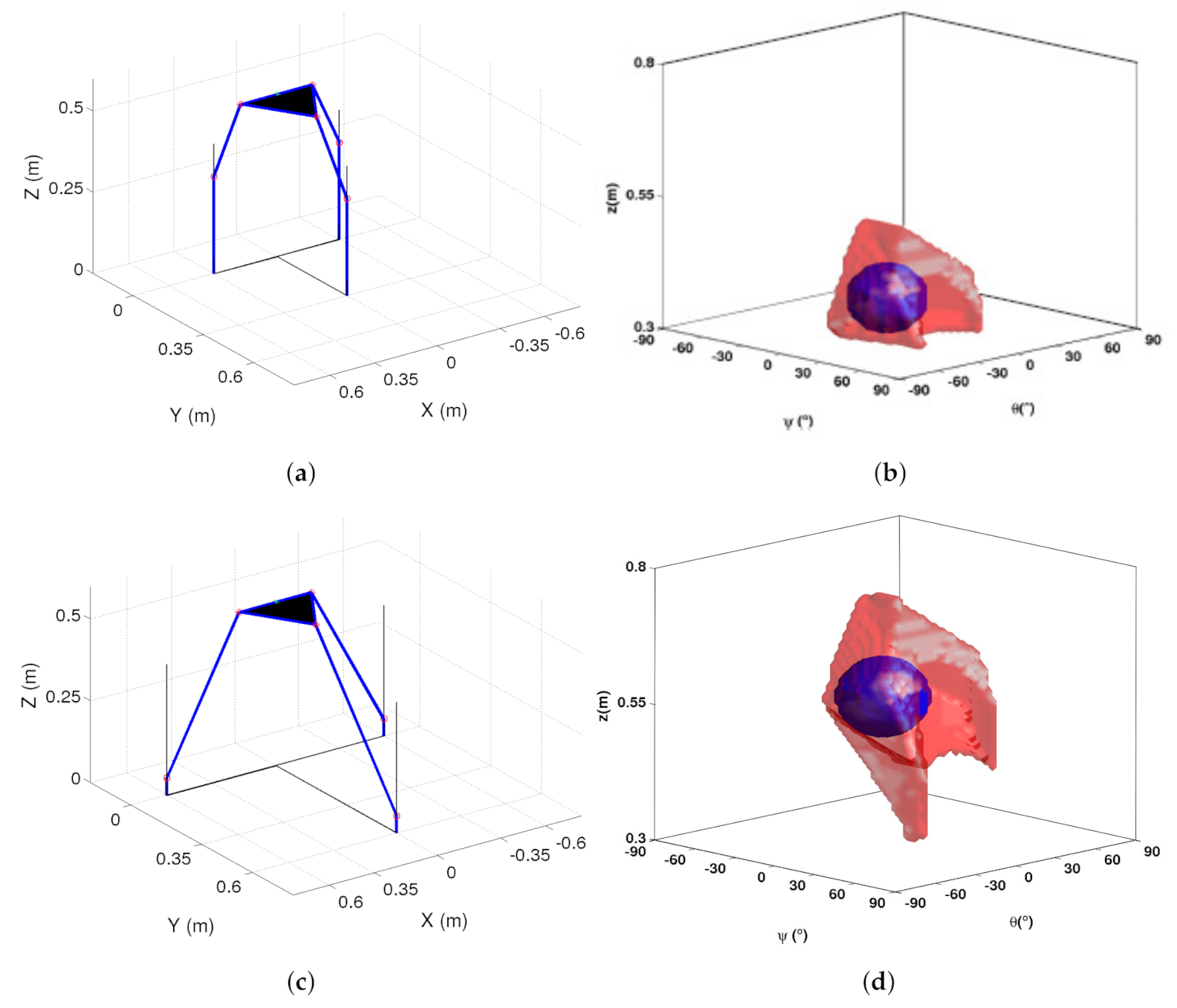
Figure 5, the 2PRU-1PRS manipulator can have two configurations depending on the relation between the value of the radius of the mobile platform and the radius of the fixed platform.
Figure 5a shows the configuration with the radius of the mobile platform smaller than the radius of the fixed platform, while
Figure 5b shows the configuration with the radius of the mobile platform bigger than the fixed one. In this work, we study the first configuration; thus, the
StudyVariables have to fulfill the condition H > R.
Since H, L and R form a triangle, they must satisfy the triangle in equality. That is, the sum of the values of the radius of the mobile platform and the length of the limbs has to be greater than the radius of the fixed platform, H < L + R. Thus, there are two conditions that we have to apply when defining the suitable GP combinations:
- i
The radius of the mobile platform is smaller than the radius of the fixed platform, R < H;
- ii
The sum of the radius of the mobile platform and the length of the limbs is larger than the radius of the fixed platform R + L > H.
By applying these restrictions, we obtain only 529 suitable GP combinations. The number of GP combinations to check has thus been reduced by 47.1% from the 1000 initial GP combinations to the 529 suitable GP combinations.
Similarly, we obtain the
. The workspace represents the poses that the the end-effector of the manipulator can reach. In this case, since our outputs are two rotations and one translation, the points in the workspace will be defined by the translation along Z-axis and the rotations about X and Y axes. Thus,
StudyPoints is the set of points which lie in the three-dimensional space bounded by the ranges given by
Table 2. We discretize each axis into 60 points, obtaining a cubic grid of size 60 × 60 × 60. Therefore, the total number of
is 216,000. We also define the ranges of the linear guides (LG) and the spherical joint (SJ) as seen in
Table 3.
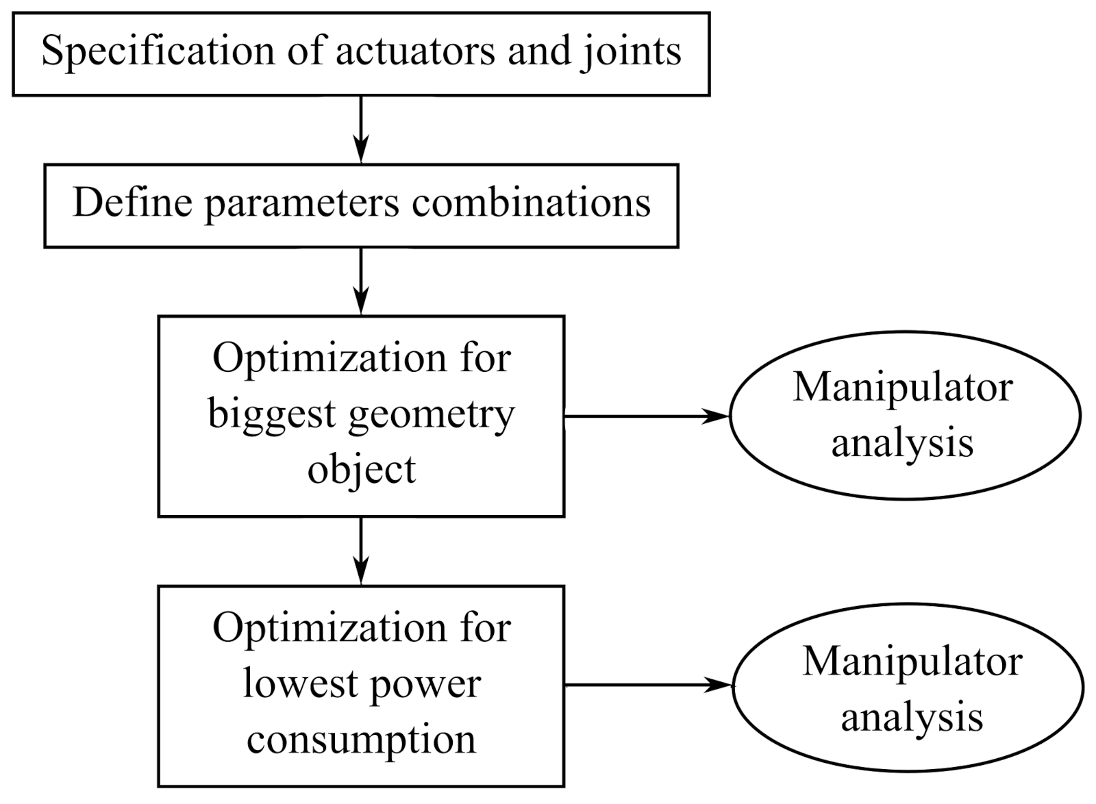
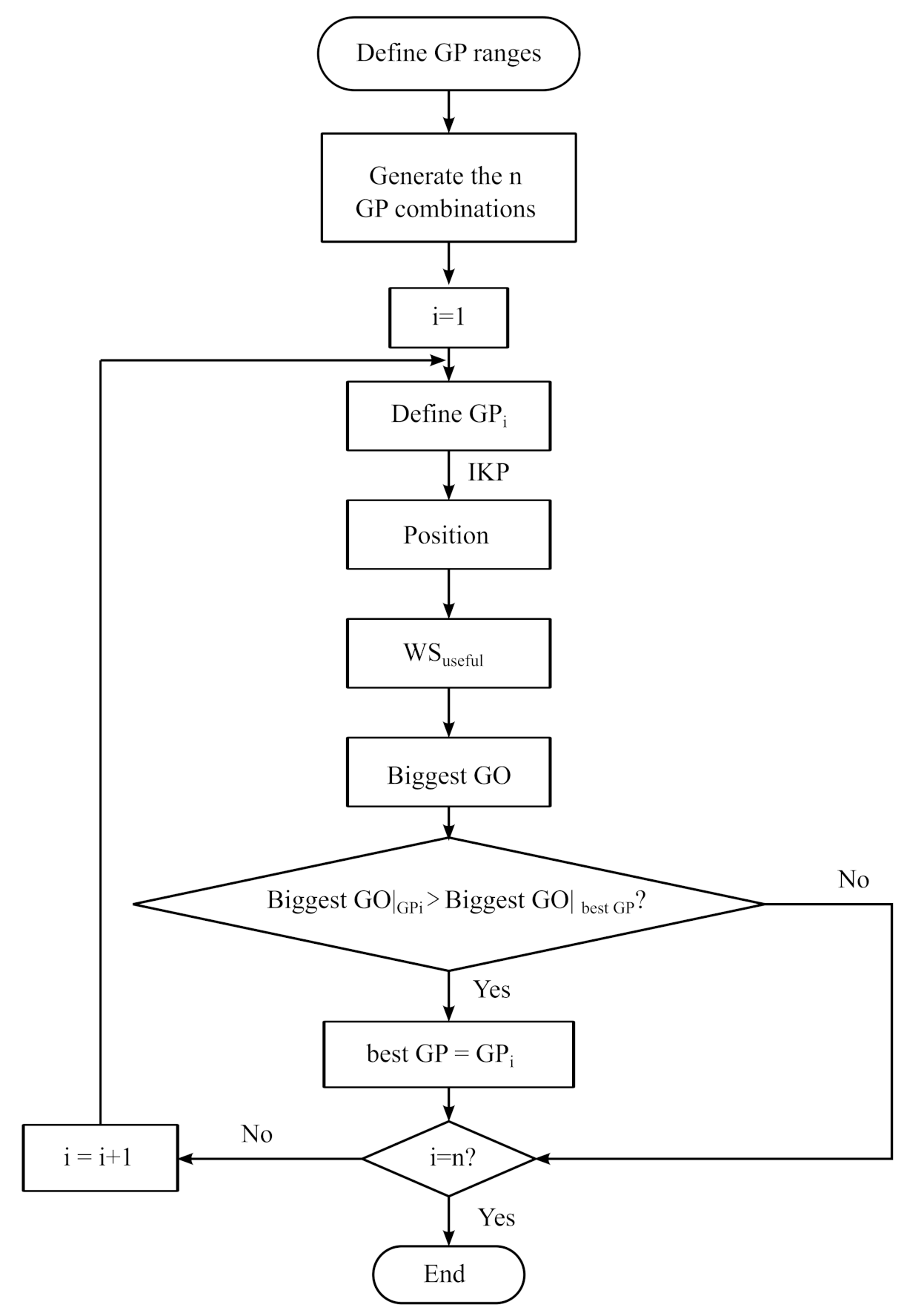
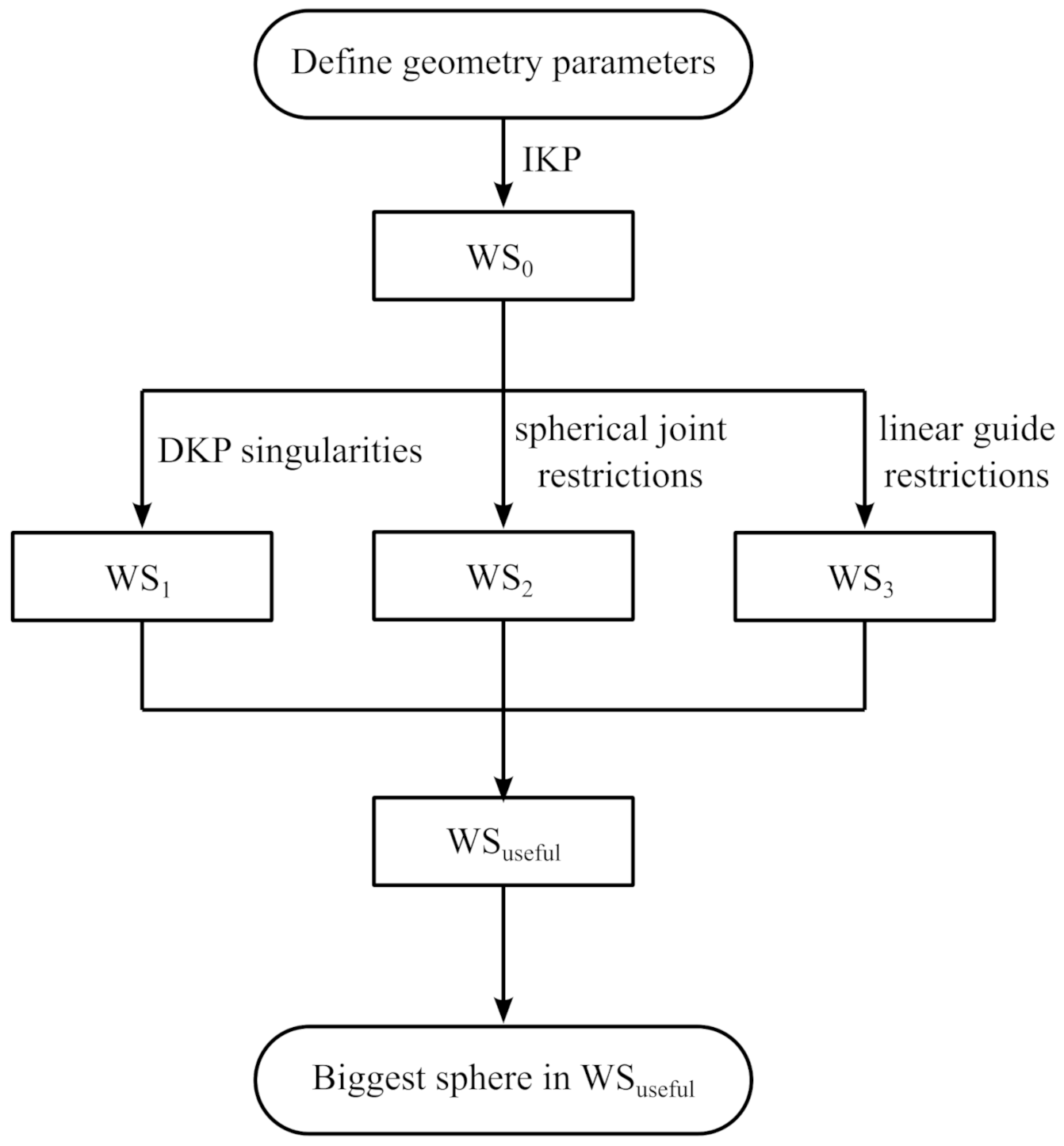
In order to have an idea of the regularity of the useful workspace and be able to determine which solution is the best one, we obtained the useful workspace and the biggest sphere in it for each suitable GP combination. The useful workspace denotes the region of the workspace free of singularities of the inverse and direct kinematic problems and where, additionally, the physical restrictions of the spherical joint and the linear guides are fulfilled. As already mentioned, we will also study the regularity of the useful workspace by obtaining the biggest sphere in it.
Figure 6 shows the steps we will follow to obtain the useful workspace of the manipulator and the biggest sphere (S
) in it for each GP combination.
For each GP combination, we first solve the inverse kinematic problem for all the candidate-poses for the workspace, and we obtain the value of the linear guides. If those solutions are imaginary, they are not possible solutions for our workspace. We define this workspace as
. We next check which points of
are in the region free of singularities and fulfill the restrictions of the spherical joint and the linear guides. The calculation of the inverse kinematic problem and the singularities is presented in Herrero et al. [
24].
When a manipulator is in a singularity of the inverse kinematic problem, the end-effector is stuck and it cannot move in the direction of the 3DOF. Mathematically, singularities related to the inverse kinematic problem appear when the determinant of the Jacobian matrix
is null: Equation (
9), as explained by Merlet [
3], Macho et al. [
26], Altuzarra et al. [
27] and Gosselin and Angeles [
28]. In practice, these singularities appear on the boundary of the workspace. We obtain the singularities of the 2PRU-1PRS PM.
When the manipulator reaches a singularity of the direct kinematics problem, it will be able to move in an infinitesimal way without changing the value of the inputs. In other words, some degrees of freedom become uncontrollable. Mathematically, this happens when the determinant of the Jacobian matrix
is null: Equation (
10) [
3]. We define
as the Jacobian matrix determinant of the direct kinematic problem in the initial mobile platform position. For a workspace free of singularities of the direct kinematic problem,
of all the points of the workspace must have the same sign. Thus, the Jacobian matrix determinant must have the same sign as
[
26,
27,
28,
29]. The set of points that fulfills this condition defines the
workspace.
The range of rotation of spherical joints is very limited. We have defined a range of since it is one of the biggest ranges we can find in commercial spherical joints. denotes the set of points of the that fulfill the spherical joint restriction.
By solving the inverse kinematic problem, we obtain the values of the linear guides for all the
StudyPoints. We checked if those values fulfill the limits of the real linear guides. Since in our case the linear guides have a displacement (
) from 0 to
m, linear guides have to fulfill Equation (
11):
where
and
.
Accordingly, we define the useful workspace as the set of points that fulfill all the previous conditions and obtain the biggest sphere that fits in each useful workspace.
Since StudyPoints are a uniform grid, we can define the “diameter of a sphere” in StudyPoints space to be number of points along the diameter.
We denote by S the largest sphere from the obtained set. The best GP combination is the one that results in the useful workspace containing the S. Note that we can have multiple useful workspace that contain the S. In that case, the best GP combination is the one that results in the S that can be placed in the most number of positions.
For these set ranges, S
has a radius of seven discretization points.
Table 4 shows the GP combinations that result in the useful workspace containing the S
and the number of positions where it can be placed.
As we can observe, there are 15 GP combinations that result in a useful workspace containing the S
. For six of those combinations, the center of the S
can be placed in two different positions, while it can be placed in four different positions for the other nine. Thus, there are nine best GP combinations given by
Table 5.
Figure 7 shows two of the best solutions and their useful workspace containing the S
placed in the first possible position. As we can observe, even if the biggest sphere is of the same size and it can be placed in the same number of places; the solution for the manipulator as well as the shape and position of the useful workspace can be very different.
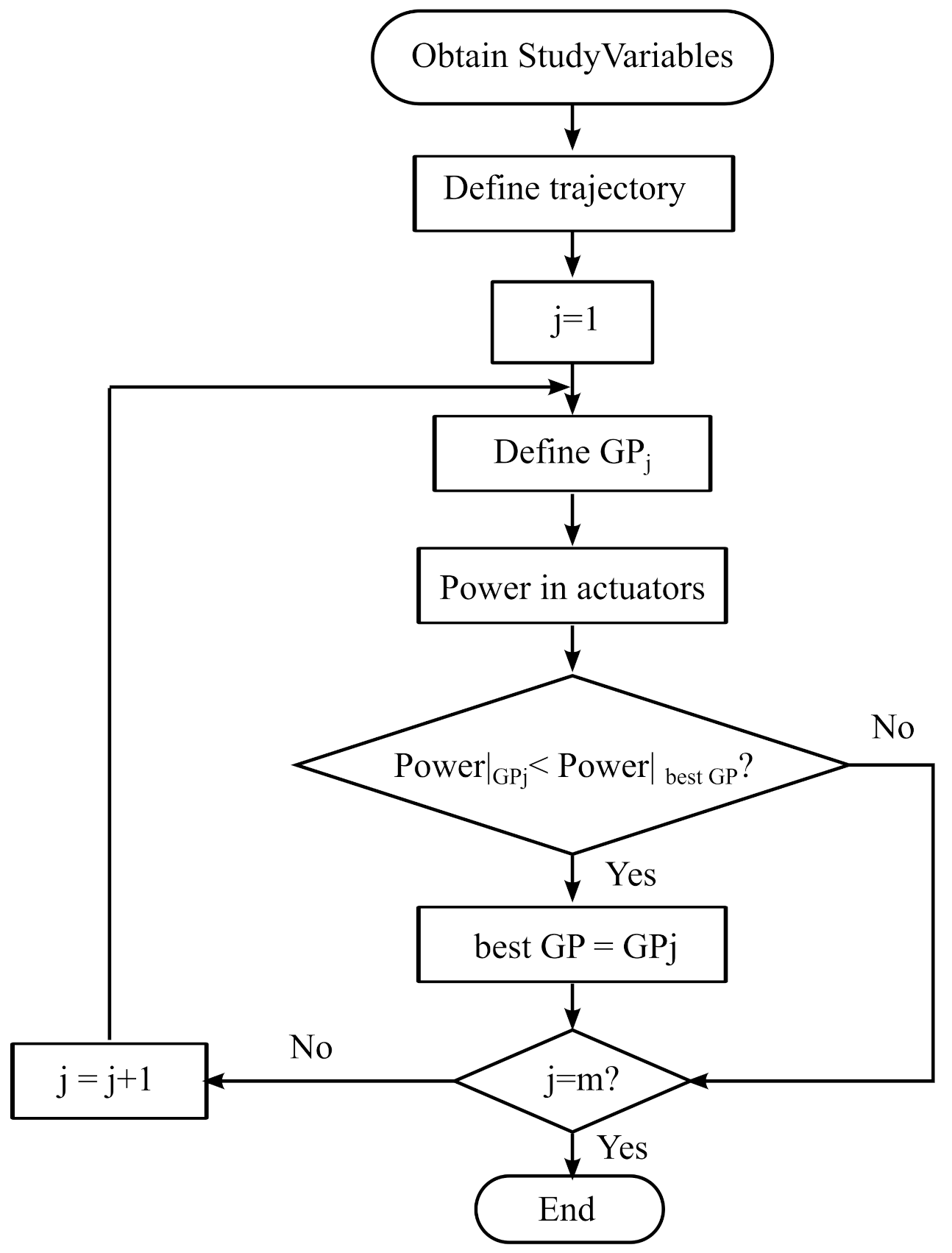
4.2. Minimize the Power Consumption
In this second algorithm, we optimize the suitable GP combinations for which the sphere contained in the useful workspace is at least 0.5·S. The suitable GP combinations that fulfill this restriction are the StudyVariables that will be considered for the power consumption optimization. In our case there are 325 StudyVariables combinations in total.
We fix the radius of the limbs and the thickness of the mobile platform. Even if these two parameters affect power consumption, in this method we only optimize the StudyVariables obtained by solving the optimization of the workspace: The optimization variables in our case will continue being H, L and R. In case we wanted to optimize the thickness of the mobile platform and the radius of the legs, the procedure would be similar, but the computational cost would increase considerably. To solve the dynamics, we also have to define the density of each component of the manipulator. We consider the material of the mobile platform to be aluminum and the material of the limbs to be steel. We chose the radius of the limbs to be m and the thickness of the mobile platform to be m.
The motors are Maxon DC Motors, with graphite brushes and a maximum power of 150 Watt. We attach to them a Maxon Planetary GP 42 C with a reduction ratio of 15. The guides we use are IGUS toothed belt linear guides.
A GP combination is suitable in the optimization of the power consumption for a given trajectory when it fulfills all the restrictions of the linear guides, motors and the gear head. According to this, in order to be a suitable GP combination for the optimization of the power consumption for a given trajectory, a GP combination has to fulfill the following conditions:
- i
The displacement of the linear guides has to be in their displacement range: 0 < < 0.3 m.
- ii
The velocity of the linear guides has to be lower than their velocity limit: d < 5 m/s.
- iii
The radial load in the linear guides has to be lower than the maximum radial load: F < 300 N.
- iv
The axial load in the linear guides has to be lower than the maximum belt tension: F < 200 N.
- v
The speed of the motors have to be lower than the maximum speed allowed: Speed
< 12,000 rpm. The expression that gives the speed of the motors is Equation (
12):
where R
is the radius of the gearhead and we obtain it by applying Equation (
13).
- vi
The power required by the motors has to be lower than the maximum power: Pow
< 150 W. We calculate the power that the motors consume by applying Equation (
14).
- vii
The torque supported by the motors cannot exceed the maximal possible torque: T
< 0.177 Nm. We obtain the torque in the motors by solving Equation (
15).
We check these criteria for each
StudyVariables and obtain the
suitable GP combinations for the power optimization process. We calculate the total power consumption during the studied trajectory for each
suitable GP combination. The power consumption of one motor over the trajectory is obtained by integrating the power required by the motor overtime, as shown in Equation (
16). Equation (
17) gives the expression of the total power consumption, which is the sum of the power consumption of the three actuators.
We define the best GP combination in terms of power consumption as the
suitable GP combination that requires the lowest power consumption for the trajectory analysed. The power consumption depends on the trajectory of the mobile platform; thus, we have different solutions of best GP combination for different trajectories. These trajectories have to be chosen according to the desired application of the manipulator. In this work, we optimized the manipulator for the three harmonic trajectories given in
Table 6: one rotation about X-axis, one rotation about Y-axis and one translation along Z-axis. We set the total time of the trajectory to be 4 seconds and discretize the trajectory into 500 points, with the time step being 0.008 s. We designate the frequency and the amplitude values to be the most commonly used for vehicle control vibration tests in Spain: frequency of 2.7 Hz and amplitude of 3
for the rotation trajectories and 3 mm for the translation.
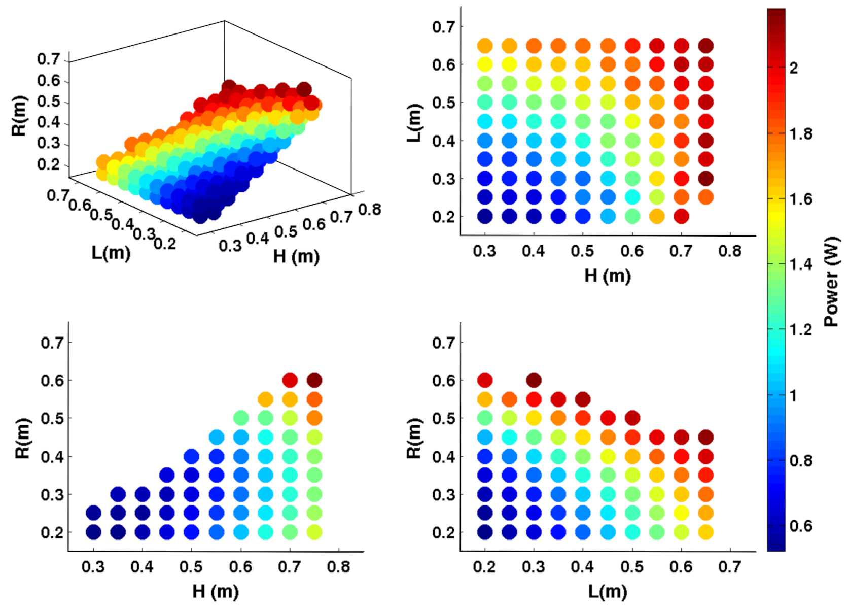
4.2.1. Translation along Z-Axis
We solve the inverse kinematic and dynamic problems for the translation along Z-axis and check that all the
StudyVariables are suitable GP combinations in this case. We obtain the total power consumption for each suitable GP combination and observe that the GP combination that consumes the highest power is (H, L, R) = (0.75, 0.3, 0.6) m: it consumes a total power of 2.1812 W. For this trajectory, we have two best GP combinations: (H, L, R) = (0.35, 0.2, 0.2) m and (H, L, R) = (0.3, 0.2, 0.2) m. Both combinations consume a total power of 0.5224 W.
Figure 8 shows the power consumption for each suitable GP combination.
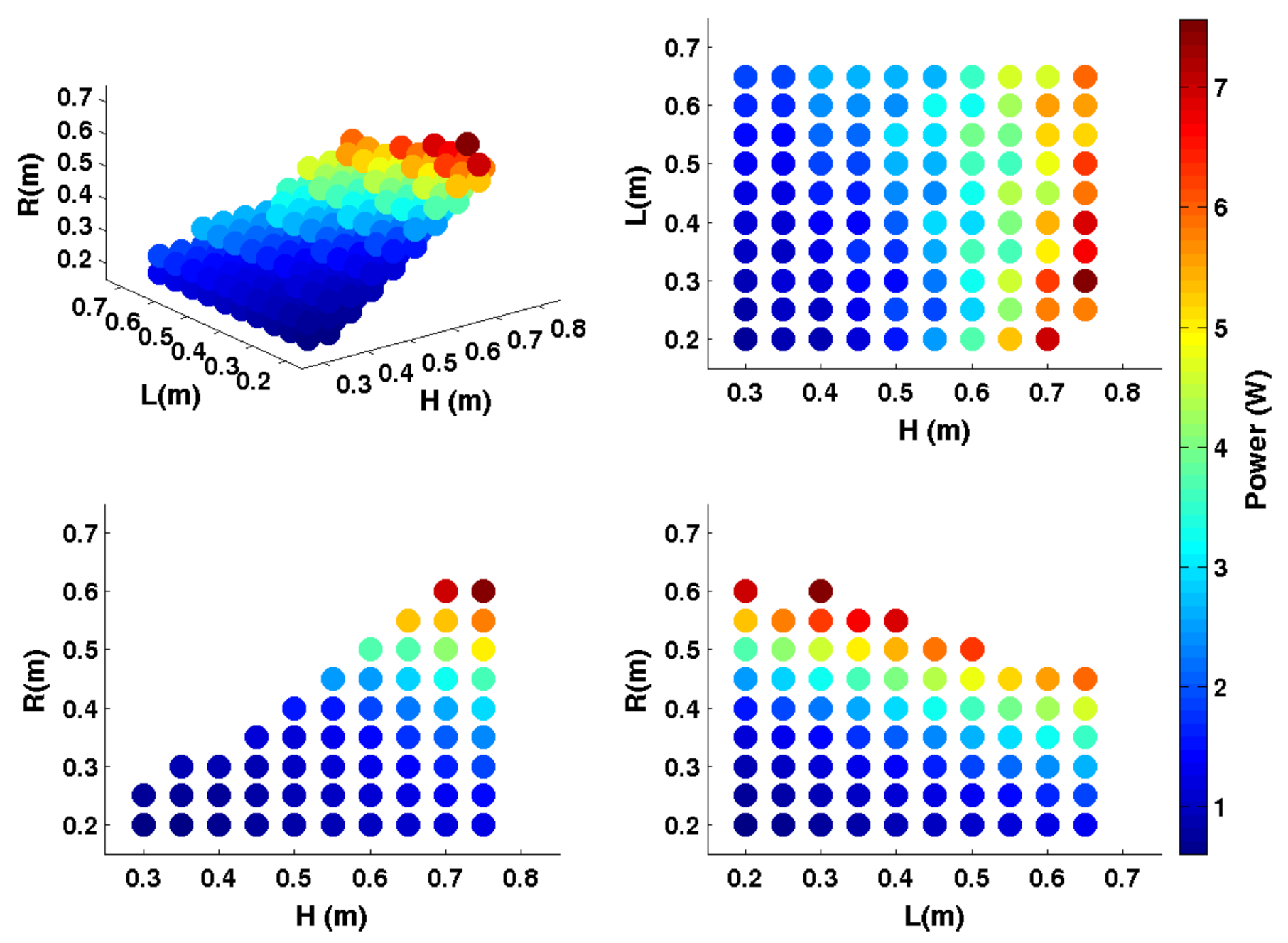
4.2.2. Rotation about X-Axis
We solve the inverse kinematic and dynamic problems for the
StudyVariables. We observe that the 325
StudyVariables fulfill the requirements of the motors and the linear guides and they are, thus, suitable GP combinations.
Figure 9 shows the total power consumption for all the suitable GP combinations for the rotation about X-axis. The GP combination (H, L, R) = (0.75, 0.3, 0.6) m is the combination that consumes the most for this trajectory: 7.5687 W. The lowest power consumption is 0.683 W and it corresponds to the GP combination (H, L, R) = (0.35, 0.2, 0.2) m. Thus, (H, L, R) = (0.35, 0.2, 0.2) m is the best GP combination for the rotation about X-axis.
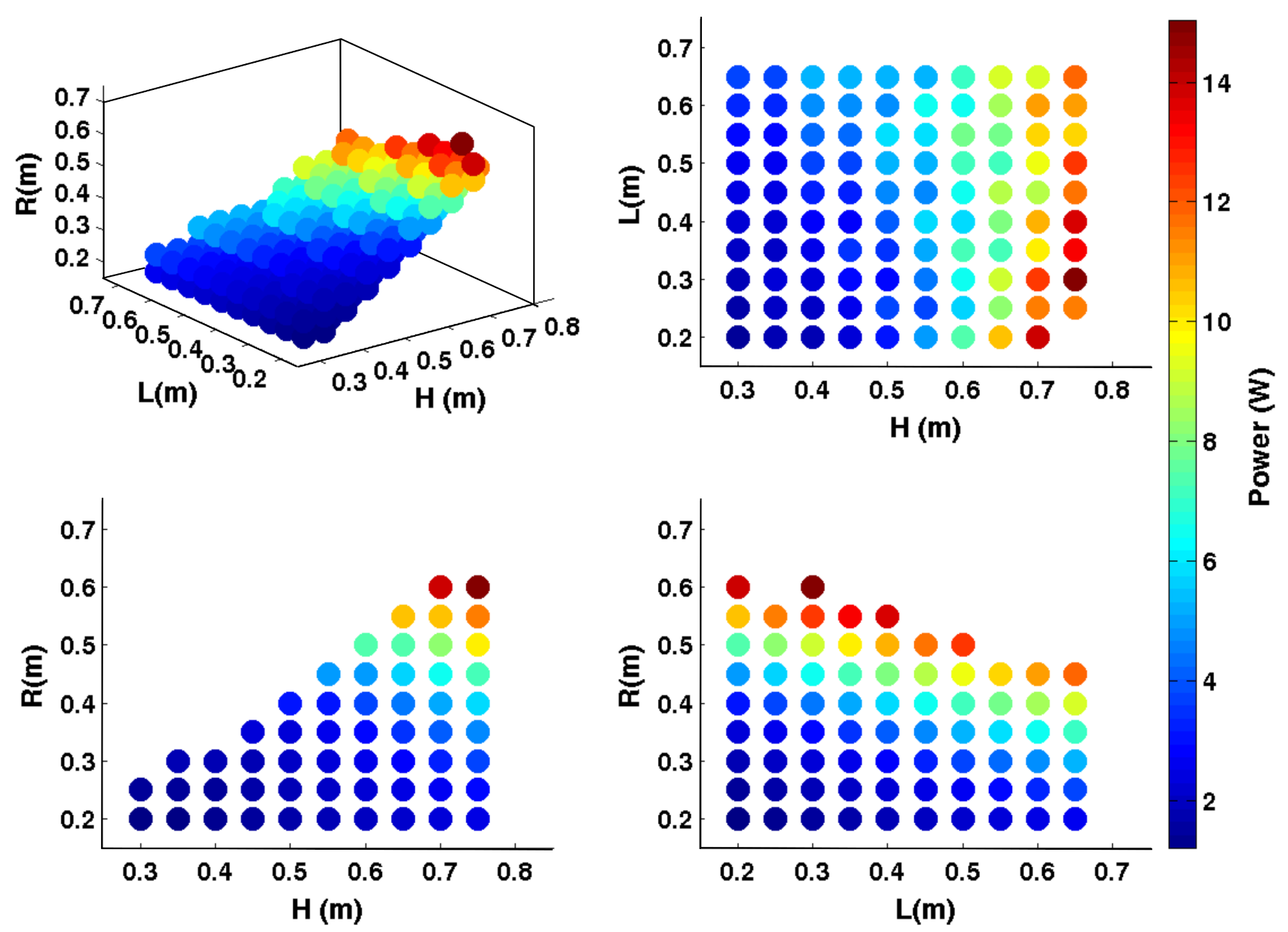
4.2.3. Rotation about Y-Axis
We checked if the
StudyVariables fulfill the restrictions of the linear guides and motors and observed that all of them are suitable GP combinations. We obtained the total power consumption for all the suitable GP combinations during the harmonic trajectory about Y-axis, and it can be observed in
Figure 10. In this case, the highest total power consumption is 15.0413 W, corresponding to the GP combination (H, L, R) = (0.75, 0.3, 0.3) m. The lowest total power consumption is 1.2133 W, the best GP combination for the rotation about Y-axis, (H, L, R) = (0.35, 0.2, 0.2) m.


