Positioning Parameter Determination Based on Statistical Regression Applied to Autonomous Underwater Vehicle

Abstract

The underwater environment is complex and changeable, and it is hard but irreplaceable to research the time-varying noises that have a significant influence on navigation information determination with higher accuracy. To solve the problems of the inaccurate noise information, this paper proposes a novel statistical regression adaptive Kalman filtering (SRAKF) algorithm that makes better use of the merits of the expectation maximization and unscented transformation. The SRAKF is verified from theoretical perspectives, and meanwhile, the stability and accuracy of the algorithm are evaluated by real lake trials. Relying on the properties of the statistical linear regression and the positioning parameter estimation of latent variables, higher precise positioning parameters can be acquired by the SRAKF, even for the measurement noise values with great variation. Hence, the performance of SRAKF is more useful in underwater positioning applications than other traditional algorithms due to its stronger robustness and higher accuracy.

1. Introduction

The ocean has become an underdeveloped high-tech resource, and it’s development has always been the strategic goal of all countries [1,2]. The autonomous underwater vehicle (AUV) plays an indispensable role in surveying, underwater reconnaissance, and underwater monitoring in the ocean. Positioning and navigation methods with higher accuracy are necessities for the AUV, as are key technologies to ensure a safe return and safe underwater work [3,4]. For one thing, there are all kinds of noise interferences in the ocean, such as salt cliffs, ocean currents, and so on, so it is hard to make an accurate underwater noise model [5]. Moreover, plenty of navigation methods based on electromagnetic propagation cannot be employed because of this signal rapidly decays underwater [6]. Additionally, the positioning error accumulation of the micro-electro-mechanical System (MEMS) [7,8,9,10] is very serious with time. Those above shortcomings will lead to bigger measurement errors, which have negative effects on AUV positioning [11]. Hence, it is important that estimation algorithms work as they are intended for AUVs [12].

The extended Kalman filter (EKF) is employed in the nonlinear system by means of the linearization approach. However, the truncated error is introduced in the nonlinear model when using the Taylor series expansion [13,14,15,16,17,18,19]. When the nonlinearity of system is extremely strong, the filter performs poorly because of the truncated error. Hence, the problem of the truncated error is solved by using the unscented transformation in the unscented Kalman filter (UKF) [20,21,22]. The UKF is more suitable than EKF for MEMS grade inertial navigation systems (INS) [23,24,25]. Additionally, it is difficult for INS to describe precise noise information due to the fact that the performance of the sensors varies in the underwater environment [26,27]. The expectation–maximization (EM) method has the advantage of simplicity, and each iteration of the EM method increases the similarity until a suboptimal solution is achieved [28,29,30]. The EM method is different from other traditional optimization methods, and it is not necessary to calculate a partial derivative. Moreover, it is not essential to be concerned about setting the iteration number [31,32,33,34,35,36]. Therefore, the EM method is an ideal adaptive method to estimate precise noise information.

A novel statistical regression adaptive Kalman filtering (SRAKF) is proposed by making use of the EM method and UKF so that the state vector of the AUV is estimated more accurately by UKF, and the EM method can help to calculate the suboptimal solution of the unknown parameters in the state–space model. The proposed SRAKF in this paper has better robustness and higher estimation accuracy, especially in the unknown and complex underwater environment.

The novelties are shown as follows:

(a)

The average absolute error is used as the criterion discard or replacement, so the data is smoothed by the combination of mean filtering and linear smoothing;

(b)

The positioning accuracy is improved by SRAKF that can calculate the accurate solutions of the predicted error covariance matrix and measurement noise matrix;

(c)

The unscented transformation is used to calculate the nonlinear integral operation. This method is conductive to increasing the state estimation accuracy by suppressing the truncation error caused by numerical integration.

The structure of the paper is shown below. The underwater positioning error model is described and presents a method to reject the outlier data in Section 2. In Section 3, the new proposed algorithm is described in detail, and the convergence property of the SRAKF is proved. Section 4 uses real experiments to show a dramatic advance in the SRAKF’s performance over UKF and CKF. The main conclusions are summarized in the last section.

2. Problem Statement and Preliminaries

The underwater positioning error model is denoted in Equation (1) [37]. In this paper, the positions calculated by high-accuracy reference navigation system are reference information.

$$\{\begin{array}{l}\delta \dot{L}=\frac{1}{R_M+h}\delta V_N-\frac{V_N}{{\left(R_M+h\right)}^2}\delta h+{\omega }_L\\ \delta \dot{\lambda }=\frac{\delta V_E\sec L}{R_N+h}+\frac{V_E\sec L\tan L}{R_N+h}\delta L+\frac{V_E\sec L}{{\left(R_N+h\right)}^2}\delta h\\ \delta \dot{h}=\delta V_U+{\omega }_h\end{array}+{\omega }_{\lambda }$$

(1)

where $\lambda$, $L$, and $h$ indicate the longitude, latitude, and height of the AUV, respectively; $V_N$, $V_E$, and $V_U$ are the velocities of the AUV along the north, east, and upward directions, respectively; $\delta L=L_{INS}-L_{\mathrm{Ref}}$, $\delta \lambda ={\lambda }_{INS}-{\lambda }_{\mathrm{Ref}}$, and $\delta h=h_{INS}-h_{\mathrm{Ref}}$ are the latitude, longitude, and height errors, respectively; $L_{INS}$ and $L_{\mathrm{Ref}}$ denote the latitudes of the AUV measured by the INS and the reference system, respectively; ${\lambda }_{INS}$ and ${\lambda }_{\mathrm{Ref}}$ are the longitudes of the AUV measured by the INS and the reference system, respectively; $h_{INS}$ and $h_{\mathrm{Ref}}$ denote the heights of the AUV measured by the INS and the reference system, respectively; $\delta V_E=V_E^{INS}-V_E^{\mathrm{Ref}}$, $\delta V_N=V_N^{INS}-V_N^{\mathrm{Ref}}$, and $\delta V_U=V_U^{INS}-V_U^{\mathrm{Ref}}$ are the velocity errors in three directions; $V_E^{INS}$ and $V_E^{\mathrm{Ref}}$ are the east velocities of the AUV measured by the INS and the reference system, respectively; $V_N^{INS}$ and $V_N^{\mathrm{Ref}}$ are the north velocities of the AUV measured by the INS and the reference system, respectively; $V_U^{INS}$ and $V_U^{\mathrm{Ref}}$ are the upward velocities of the AUV measured by the INS and the reference system, respectively; $R_N$ and $R_M$ are the long and short axis radii of the earth; ${\omega }_L$, ${\omega }_{\lambda }$, and ${\omega }_h$ are the process noises on three axes.

Equation (1) can be rewritten as the state–space model, shown in Equation (2).

$$\left[\begin{array}{c}\delta \dot{L}\\ \delta \dot{\lambda }\\ \delta \dot{h}\end{array}\right]=FX+u+\mathsf{\omega }=\left[\begin{array}{ccc}0& 0& -\frac{V_N^n}{{\left(R_M+h\right)}^2}\\ \frac{V_E^n\sec L\tan L}{R_N+h}& 0& \frac{V_E^n\sec L}{{\left(R_N+h\right)}^2}\delta h\\ 0& 0& 0\end{array}\right]\left[\begin{array}{c}\delta L\\ \delta \lambda \\ \delta h\end{array}\right]+\left[\begin{array}{c}\frac{\delta V_N}{R_M+h}\\ \frac{\delta V_E\sec L}{R_N+h}\\ \delta V_U\end{array}\right]+\left[\begin{array}{c}{\omega }_L\\ {\omega }_{\lambda }\\ {\omega }_h\end{array}\right]$$

(2)

where $X={\left[\begin{array}{ccc}\delta L& \delta \lambda & \delta h\end{array}\right]}^T$ is the state vector; $u={\left[\begin{array}{ccc}\frac{\delta V_N}{R_M+h}& \frac{\delta V_E\sec L}{R_N+h}& \delta V_U\end{array}\right]}^T$ is the input information; $\mathsf{\omega }={\left[\begin{array}{ccc}{\omega }_L& {\omega }_{\lambda }& {\omega }_h\end{array}\right]}^T$ is the process noise; $Q$ is the process noise covariance matrix; the process noise is assumed to follow the Gaussian distribution with zero means and the covariance matrix $Q$; $k$ is the time of $k$.

The state transition matrix $F_{k|k-1}$ is approximated as follows:

$$F_{k|k-1}\approx I_n+F\mathsf{\Delta }\mathrm{t}$$

(3)

where $n$ denotes the dimension of the state vector; $I_n$ is the identity matrix of the $n$ dimensions; $\mathsf{\Delta }\mathrm{t}$ is the time interval.

The measurement function is shown as follows:

$$Z=HX+v=\left[\begin{array}{c}{L}^{INS}-L^{\mathrm{Ref}}\\ {\lambda }^{INS}-{\lambda }^{\mathrm{Ref}}\\ h^{INS}-h^{\mathrm{Ref}}\end{array}\right]=\left[\begin{array}{ccc}1& 0& 0\\ 0& 1& 0\\ 0& 0& 1\end{array}\right]\left[\begin{array}{c}\delta L\\ \delta \lambda \\ \delta h\end{array}\right]+\left[\begin{array}{c}{\mathrm{v}}_L\\ {\mathrm{v}}_{\lambda }\\ {\mathrm{v}}_h\end{array}\right]$$

(4)

where $Z$ represents the measurement vector; $H=I_3$ represents the measurement transformation matrix; $v={\left[\begin{array}{ccc}{\mathrm{v}}_L& {\mathrm{v}}_{\lambda }& {\mathrm{v}}_h\end{array}\right]}^T$ is the measurement noise; ${\mathrm{v}}_L$, ${\mathrm{v}}_{\lambda }$, and ${\mathrm{v}}_h$ are the measurement noises on the three axes, respectively; $R$ is the measurement noise matrix; the measurement noise is assumed to follow the Gaussian distribution with zero mean and the covariance matrix $R$.

Remark 1:

The tri-axis MEMS accelerometers, tri-axis MEMS gyroscopes, and tri-axis magnetometers are used to collect data.

$$\mathsf{\Lambda }=\left\{x_1,x_2,\dots ,x_k\right\}$$

(5)

where $x_k$ is the sampled data at time $k$. However, it is unavoidable that there will be outliers in the sampled data. In order to eliminate the outliers, linear smoothing is used to remove the outliers. First, the average absolute error $\tilde{Z}$ is derived by Equation (6):

$$\tilde{Z}=\left({\displaystyle \sum _{i=1}^{k-1}|z_i|}\right)/k-1$$

(6)

where the absolute error $z_i$ is defined as follows:

$$z_i=x_{i+1}-x_i,i=1,2,\dots ,k-1$$

(7)

Criterion: 

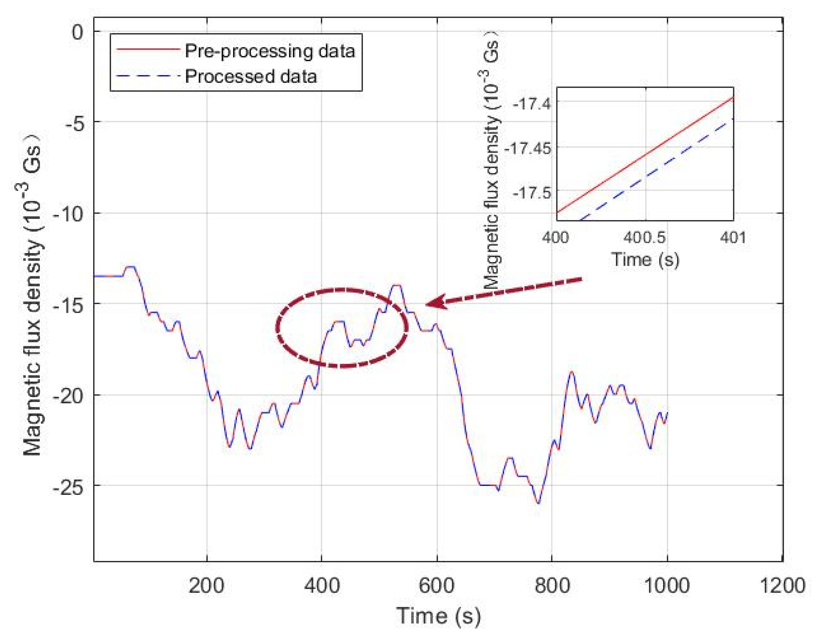
The data $x_{i+1}$ is retained if $z_i<\tilde{Z}$, or the outliers are replaced by a mean function $z_i=\frac{\stackrel{2m}{\overbrace{(z_{i-m}+\dots +z_{i-1}+z_{i+1}+\dots +z_{i+m})}}}{2m}$. Figure 1 shows the effect of data processing. The data comparisons (accelerometer, gyroscope, and magnetometer) between the pre-processing and processed data are shown in Figure 1, Figure 2 and Figure 3.

In order to quantitatively compare the processed data with the pre-processing data, the root mean square error (RMSE) is used here:

$$\mathrm{RMSE}=\sqrt{{\displaystyle \sum _{i=1}^{k-1}{(z_i-\tilde{Z})}^2}}/(k-1)$$

(8)

where Acce, Gyro, and Mag are the abbreviations for the acceleration sensors, gyroscope sensors, and magnetic sensors, respectively.

The RMSE values obtained using data processing method are calculated in

Table 1. Comparison of the RMSE for pre-processing data and processed data.

	Pre-Processing Data			Processed Data
Sensors	Acce	Gyro	Mag	Acce	Gyro	Mag
RMSE	0.1260	0.0035	0.0076	0.0886	0.0026	0.0051

. It can be seen that the probability of the outliers decreased by 29.68% for the accelerometer, by 25.71% for the gyroscope, and by 32.89% for the magnetometer.

The average absolute error shown in Equation (6) is as the criterion. The raw data is observed if the data meets this criterion, or else the raw data is thought of as the outlier and should be deleted. When the outlier is rejected, the points near the outliers are averaged to smooth the data. Therefore, it not only eliminates the outliers but also describes the accurate characteristics for the raw data. The proposed rejection method has better denoising performance.

3. The Statistical Regression Adaptive Kalman Filtering Algorithm

Set ${\mathsf{\Phi }}_k\triangleq \left\{\begin{array}{cc}{P}_{k|k-1}& R_k\end{array}\right\}$, then the maximum likelihood estimation (MLE) of ${\mathsf{\Phi }}_k$ is written as ${\widehat{\mathsf{\Phi }}}_k$, which is described as follows:

$${\widehat{\mathsf{\Phi }}}_k=\arg \underset{{\mathsf{\Phi }}_k}{\max }{p}_{{\mathsf{\Phi }}_k}(Z_{1:k})=\arg \underset{{\mathsf{\Phi }}_k}{\max }\log p_{{\mathsf{\Phi }}_k}(Z_{1:k})$$

(9)

where $p_{{\mathsf{\Phi }}_k}(•)$ is the probability density function (PDF) related to the parameter ${\mathsf{\Phi }}_k$. Nevertheless, $p_{{\mathsf{\Phi }}_k}(Z_{1:k})$ cannot be obtained because $Z_k$ depends on $X_{k|k}$, which is unknown. Then, the minimum variance estimation $\mathsf{\Omega }({\mathsf{\Phi }}_k,{\mathsf{\Phi }}_k^{\left(l\right)})$ is used to approximate $\log p_{{\mathsf{\Phi }}_k}(X_{k|k},Z_{1:k})$.

$$\begin{array}{c}{L}_{{\mathsf{\Phi }}_k}(X_{k|k},Z_{1:k})\doteq \mathsf{\Omega }({\mathsf{\Phi }}_k,{\mathsf{\Phi }}_k^{\left(l\right)})\\ \hspace{1em}\hspace{1em}\hspace{1em}\hspace{1em}\hspace{1em}\hspace{1em}\hspace{1em}\hspace{1em}\hspace{1em}\hspace{1em}\hspace{1em}\hspace{1em}\hspace{1em} =E_X[\log p_{{\mathsf{\Phi }}_k}(X_{k|k},Z_{1:k})|{\mathsf{\Phi }}_k^{\left(l\right)},Z_{1:k}]\\ \hspace{1em}\hspace{1em}\hspace{1em}\hspace{1em}\hspace{1em}\hspace{1em}\hspace{1em}\hspace{1em}\hspace{1em}\hspace{1em}\hspace{1em}\hspace{1em}\hspace{1em}\hspace{1em}\hspace{1em}\hspace{1em}\hspace{1em}={\displaystyle \int \log }{p}_{{\mathsf{\Phi }}_k}(X_{k|k},Z_{1:k})p_{{\mathsf{\Phi }}_k^{\left(l\right)}}(X_{k|k}|Z_{1:k})d{X}_{k|k}\end{array}$$

(10)

where $E_X[•]$ is an expectation of $X_{k|k}$; ${\mathsf{\Phi }}_k^{\left(l\right)}$ is an approximate solution of ${\widehat{\mathsf{\Phi }}}_k$ at the $l$th iteration; $\mathsf{\Omega }({\mathsf{\Phi }}_k,{\mathsf{\Phi }}_k^{\left(l\right)})$ is defined as the conditional expectation of $\log p_{{\mathsf{\Phi }}_k}(X_{k|k},Z_{1:k})$.

3.1. The Expectation Approach

$\log p_{{\mathsf{\Phi }}_k}(X_{k|k},Z_{1:k})$ is factored using Equation (11):

$$\begin{array}{c}\log p_{{\mathsf{\Phi }}_k}(X_{k|k},Z_{1:k})=\log [p_{{\mathsf{\Phi }}_k}(Z_{k|k}|X_{k|k},Z_{1:k-1})p_{{\mathsf{\Phi }}_k}(X_{k|k}|Z_{1:k-1})p(Z_{1:k-1})]\\ \hspace{1em}\hspace{1em}\hspace{1em}\hspace{1em}\hspace{1em}\hspace{1em}\hspace{1em}\hspace{1em}\hspace{1em}\hspace{1em}\hspace{1em}\hspace{1em}=\log [p_{{\mathsf{\Phi }}_k}(Z_{k|k}|X_{k|k},Z_{1:k-1})]+\log [p_{{\mathsf{\Phi }}_k}(X_{k|k}|Z_{1:k-1})]+\log [p(Z_{1:k-1})]\end{array}$$

(11)

where $p_{{\mathsf{\Phi }}_k}(Z_k|X_{k|k},Z_{1|k-1})=p_{{\mathsf{\Phi }}_k}(Z_k|X_{k|k})$ because $X_{k|k}$ includes all of the information in $Z_{1:k-1}$.

Remark 2:

The predicted PDF $p_{{\mathsf{\Phi }}_k}(X_{k|k}|Z_{1:k-1})$ is approximated to follow the Gaussian distribution; then, the $2n+1$ sigma points are selected, and the moment estimation of $p_{{\mathsf{\Phi }}_k}(X_{k|k}|Z_{1:k-1})$ is calculated using the unscented transformation. The mean and covariance matrix of $p_{{\mathsf{\Phi }}_k}(X_{k|k}|Z_{1:k-1})$ with higher accuracy are acquired for the nonlinear state equation.

$$\begin{array}{c}{p}_{{\mathsf{\Phi }}_k}\left(X_{k|k}|Z_{1:k-1}\right)=\mathrm{N}\left(X_{k|k};X_{k|k-1},P_{k|k-1}\right)\\ \hspace{1em}\hspace{1em}\hspace{1em}\hspace{1em}\hspace{1em}\hspace{1em}\hspace{1em}\hspace{1em}\hspace{1em}\hspace{1em}\hspace{1em}\hspace{1em}\hspace{1em}\hspace{1em}=\mathrm{N}\left(X_{k|k};{\displaystyle \sum _{i=0}^{2n}{\omega }_m\left(i\right)F_{k|k-1}{\chi }_{i,k-1|k-1}},P_{k|k-1}\right)\end{array}$$

(12)

where $\mathrm{N}(•;\mu ,\sum )$ is the Gaussian distribution with the mean $\mu$ and covariance $\sum$.

The predicted error covariance matrix and $P_{k|k-1}$ predicted state vector $X_{k|k-1}$ are calculated as follows:

The sigma points are given using Equation (13):

$$\{\begin{array}{cc}{\chi }_{i,k-1|k-1}=X_{k-1|k-1},& i=0\\ {\chi }_{i,k-1|k-1}=X_{k-1|k-1}+{(\sqrt{(n+\rho )P_{k-1|k-1}})}_i,& i=1,\dots ,n\\ {\chi }_{i+n,k-1|k-1}=X_{k-1|k-1}-{(\sqrt{(n+\rho )P_{k-1|k-1}})}_i,& i=1,\dots ,n\end{array}$$

(13)

where $n$ means the dimension of $X_{k|k}$; $\rho$ means the scaling parameter; ${(\bullet )}_i$ is the $i$th column of the matrix; $P_{k-1|k-1}$ is the error covariance matrix at the time $k-1$.

The weight functions of the mean $W_m(i)$ and covariance matrix $W_C(i)$ are defined as follows:

$$W_m(i)=W_C(i)=\{\begin{array}{cc}\rho /(n+\rho ),& i=0\\ 1/2(n+\rho ),& i=1,\dots ,2n\end{array}$$

(14)

The predicted state vector $X_{k|k-1}$ and predicted error covariance matrix $P_{k|k-1}$ are given:

$$\{\begin{array}{l}{X}_{k|k-1}={\displaystyle \sum _{i=0}^{2n}{\omega }_m\left(i\right)F_{k|k-1}{\chi }_{i,k-1|k-1}}+u_{k-1}\mathsf{\Delta }\mathrm{t}\\ P_{k|k-1}={\displaystyle \sum _{i=0}^{2n}{\omega }_C\left(i\right)\left(F_{k|k-1}{\chi }_{i,k-1|k-1}-X_{k|k-1}\right){\left(F_{k|k-1}{\chi }_{i,k-1|k-1}-X_{k|k-1}\right)}^T}+Q_{k-1}\end{array}$$

(15)

Similarly, $p_{{\mathsf{\Phi }}_k}(Z_k|X_{k|k})$ is approximated as

$$\begin{array}{c}{p}_{{\mathsf{\Phi }}_k}\left(Z_k|X_{k|k}\right)=\mathrm{N}\left(Z_k;Z_{k|k-1},R_k\right)\\ \hspace{1em}\hspace{1em}\hspace{1em}\hspace{1em}\hspace{1em}\hspace{1em}\hspace{1em}\hspace{1em}\hspace{1em}\hspace{1em}\hspace{1em}\hspace{1em}\hspace{1em}\hspace{1em}=\mathrm{N}\left(Z_k;{\displaystyle \sum _{i=0}^{2n}{\omega }_m\left(i\right)H{F}_{k|k-1}{\chi }_{i,k-1|k-1}},R_k\right)\end{array}$$

(16)

where the predicted measurement vector $Z_{k|k-1}$ is calculated as follows:

$$\{\begin{array}{l}{Z}_{i,k|k-1}^{*}=H{F}_{k|k-1}{\chi }_{i,k-1|k-1}\\ Z_{k|k-1}={\displaystyle \sum _{i=0}^{2n}{W}_m(i)Z_{i,k|k-1}^{*}}\end{array}$$

(17)

Employing Equations (11), (12), and (16), $\log p_{{\mathsf{\Phi }}_k}(X_{k|k},Z_{1:k})$ can be deduced using Equation (18):

$$\begin{array}{c}\log p_{{\mathsf{\Phi }}_k}(X_{k|k},Z_{1:k})=-0.5{\left[Z_k-{\displaystyle \sum _{i=0}^{2n}{\omega }_m(i)H{F}_{k|k-1}{\chi }_{i,k-1|k-1}}\right]}^T{R}_k^{-1}\left[Z_k-{\displaystyle \sum _{i=0}^{2n}{\omega }_m(i)H{F}_{k|k-1}{\chi }_{i,k-1|k-1}}\right]\\ \hspace{1em}\hspace{1em}\hspace{1em}\hspace{1em}\hspace{1em}\hspace{1em}\hspace{1em}\hspace{1em} -0.5{\left[X_{k|k}-{\displaystyle \sum _{i=0}^{2n}{\omega }_m(i)F_{k|k-1}{\chi }_{i,k-1|k-1}}\right]}^T{P}_{k|k-1}^{-1}\left[X_{k|k}-{\displaystyle \sum _{i=0}^{2n}{\omega }_m(i)F_{k|k-1}{\chi }_{i,k-1|k-1}}\right]\\ \hspace{1em}\hspace{1em}\hspace{1em}\hspace{1em}\hspace{1em}\hspace{1em}\hspace{1em}\hspace{1em} -0.5\log |R_k|-0.5\log |P_{k|k-1}|+c_{{\mathsf{\Phi }}_k}\hfill \end{array}$$

(18)

where $|\bullet |$ represents the determinant operation of a matrix, and $c_{{\mathsf{\Phi }}_k}$ represents a constant value with regard to the variable ${\mathsf{\Phi }}_k$.

The posterior PDF is $p_{{\mathsf{\Phi }}_k}(X_{k|k},Z_{1:k})$ while ${\mathsf{\Phi }}_k={\mathsf{\Phi }}_k^{\left(l\right)}$ is approximated as the Gaussian PDF:

$$p_{{\mathsf{\Phi }}_k^{\left(l\right)}}\left(X_{k|k},Z_{1:k}\right)=\mathrm{N}\left(X_{k|k};X_{k|k}^{\left(l+1\right)},P_{k|k}^{\left(l+1\right)}\right)$$

(19)

where the mean and covariance of $X_{k|k}$ are $X_{k|k}^{\left(l+1\right)}$ and $P_{k|k}^{\left(l+1\right)}$. Different from the linearization method mentioned above, the unscented transformation is employed in the measurement process update. The integration calculation for the nonlinear function is transformed into the weight sum for sigma points so that the negative effect caused by the truncation error is reduced. The computational procedure is presented.

Remark 3:

The measurement error covariance matrix $P_{zz}^{\left(l\right)}$ and cross error covariance matrix $P_{xz}^{\left(l\right)}$ are calculated as follows:

$$\{\begin{array}{l}{P}_{xz}^{\left(l\right)}={\displaystyle \sum _{i=1}^{2n+1}{\omega }_c(i)\left[{\chi }_{i,k-1|k-1}^{\left(l\right)}-X_{k|k-1}\right]{\left[F_{k|k-1}{\chi }_{i,k-1|k-1}^{\left(l\right)}-X_{k|k-1}\right]}^T}\\ P_{zz}^{\left(l\right)}={\displaystyle \sum _{i=1}^{2n+1}\left\{{\omega }_c(i)\left[H{F}_{k|k-1}{\chi }_{i,k-1|k-1}^{\left(l\right)}-Z_{k|k-1}\right]{\left[H{F}_{k|k-1}{\chi }_{i,k-1|k-1}^{\left(l\right)}-Z_{k|k-1}\right]}^T\right\}}+R_k^{\left(l\right)}\end{array}$$

(20)

Then, the Kalman gain $K^{\left(l+1\right)}$ is updated:

$$K^{\left(l+1\right)}=P_{xz}^{\left(l\right)}/P_{zz}^{\left(l\right)}$$

(21)

Hence, $X_{k|k}^{\left(l+1\right)}$ and $P_{k|k}^{\left(l+1\right)}$ are deduced using Equation (22).

$$\{\begin{array}{l}{X}_{k|k}^{\left(l+1\right)}=X_{k|k-1}+K^{\left(l+1\right)}\left[Z_k-{\displaystyle \sum _{i=1}^{2n+1}{\omega }_m(i)H{F}_{k|k-1}{\chi }_{i,k-1|k-1}^{\left(l\right)}}\right]\\ P_{k|k}^{\left(l+1\right)}=P_{k|k-1}^{\left(l\right)}-K^{\left(l+1\right)}{P}_{zz}^{\left(l\right)}{\left(K^{\left(l+1\right)}\right)}^T\end{array}$$

(22)

Eventually, $\mathsf{\Omega }({\mathsf{\Phi }}_k,{\mathsf{\Phi }}_k^{\left(l\right)})$ can be simplified as

$$\mathsf{\Omega }\left({\mathsf{\Phi }}_k,{\mathsf{\Phi }}_k^{\left(l\right)}\right)=-0.5\log |R_k|-0.5tr(L_k{R}_k^{-1})-0.5\log |P_{k|k-1}|-0.5tr(J_k{P}_{k|k-1}^{-1})+c_{{\mathsf{\Phi }}_k}$$

(23)

where $tr(•)$ represents the trace operation of a matrix, $L_k$ and $J_k$ are obtained by

$$L_k={\displaystyle \int \left[Z_k-{\displaystyle \sum _{i=0}^{2n}{\omega }_m(i)H{F}_{k|k-1}{\chi }_{i,k-1|k-1}}\right]{\left[Z_k-{\displaystyle \sum _{i=0}^{2n}{\omega }_m(i)H{F}_{k|k-1}{\chi }_{i,k-1|k-1}}\right]}^T\mathrm{N}\left(X_{k|k};X_{k|k}^{(l+1)},P_{k|k}^{\left(l+1\right)}\right)d{X}_{k|k}}$$

(24)

$$J_k={\displaystyle \int \left[X_{k|k}-{\displaystyle \sum _{i=0}^{2n}{\omega }_m(i)F_{k|k-1}{\chi }_{i,k-1|k-1}}\right]{\left[X_{k|k}-{\displaystyle \sum _{i=0}^{2n}{\omega }_m(i)F_{k|k-1}{\chi }_{i,k-1|k-1}}\right]}^T\mathrm{N}\left(X_{k|k};X_{k|k}^{(l+1)},P_{k|k}^{\left(l+1\right)}\right)d{X}_{k|k}}$$

(25)

The sigma point $\vartheta$ is used to calculate the covariance matrices at the $l+1$th iteration.

$$\{\begin{array}{cc}{\vartheta }_{i,k|k}=X_{k|k}^{\left(l+1\right)},& i=0\\ {\vartheta }_{i,k|k}=X_{k|k}^{\left(l+1\right)}+{\left(\sqrt{(n+\rho )P_{k|k}^{\left(l+1\right)}}\right)}_i,& i=1,\dots ,n\\ {\vartheta }_{i+n,k|k}=X_{k|k}^{\left(l+1\right)}-{\left(\sqrt{(n+\rho )P_{k|k}^{\left(l+1\right)}}\right)}_i,& i=1,\dots ,n\end{array}$$

(26)

Similarly, $L_k$ and $J_k$ are obtained using Equations (27) and (28).

$$L_k={\displaystyle \sum _{i=0}^{2n}{\omega }_C\left(i\right)\left(Z_k-H{\vartheta }_{i,k|k}\right){\left(Z_k-H{\vartheta }_{i,k|k}\right)}^T}$$

(27)

$$J_k=P_{k|k}^{\left(l+1\right)}+\left[X_{k|k}^{\left(l+1\right)}-{\displaystyle \sum _{i=1}^{2n+1}\omega (i)F_{k|k-1}{\chi }_{i,k-1|k-1}}\right]{\left[X_{k|k}^{\left(l+1\right)}-{\displaystyle \sum _{i=1}^{2n+1}\omega (i)F_{k|k-1}{\chi }_{i,k-1|k-1}}\right]}^T$$

(28)

3.2. The Maximization Approach

The maximization step includes the maximization of $\mathsf{\Omega }({\mathsf{\Phi }}_k,{\mathsf{\Phi }}_k^{\left(l\right)})$. In order to find the extreme point, the first-order derivative of $\mathsf{\Omega }({\mathsf{\Phi }}_k,{\mathsf{\Phi }}_k^{\left(l\right)})$ should be obtained and set as equal to zero.

$$\frac{\partial \mathsf{\Omega }({\mathsf{\Phi }}_k,{\mathsf{\Phi }}_k^{\left(l\right)})}{\partial {\mathsf{\Phi }}_k}{|}_{{\mathsf{\Phi }}_k={\mathsf{\Phi }}_k^{\left(l+1\right)}}=0$$

(29)

Employing ${\mathsf{\Phi }}_k=\left\{\begin{array}{cc}{P}_{k|k-1}& R_k\end{array}\right\}$, Equation (29) can be computed as

$$\{\begin{array}{l}\frac{\partial \mathsf{\Omega }\left({\mathsf{\Phi }}_k,{\mathsf{\Phi }}_k^{\left(l\right)}\right)}{\partial P_{k|k-1}}=-\frac{1}{2}{P}_{k|k-1}^{-1}+\frac{1}{2}{P}_{k|k-1}^{-1}{J}_k{P}_{k|k-1}^{-1}=0\\ \frac{\partial \mathsf{\Omega }\left({\mathsf{\Phi }}_k,{\mathsf{\Phi }}_k^{\left(l\right)}\right)}{\partial R_k}=-\frac{1}{2}{R}_k^{-1}+\frac{1}{2}{R}_k^{-1}{L}_k{R}_k^{-1}=0\end{array}$$

(30)

Solving Equation (30), then

$$\{\begin{array}{l}{P}_{k|k-1}^{\left(l+1\right)}=J_k\\ R_k^{\left(l+1\right)}=L_k\end{array}$$

(31)

After iteration $N$, the estimations of $P_{k|k-1}$ and $R_k$ are derived as follows, respectively.:

$$\{\begin{array}{l}{P}_{k|k-1}=P_{k|k-1}^{\left(N\right)}\\ R_k=R_k^{\left(N\right)}\end{array}$$

(32)

Similarly, the estimation of $X_{k|k}$ and $P_{k|k}$ are denoted as

$$\{\begin{array}{l}{X}_{k|k}=X_{k|k}^{\left(N\right)}\\ P_{k|k}=P_{k|k}^{\left(N\right)}\end{array}$$

(33)

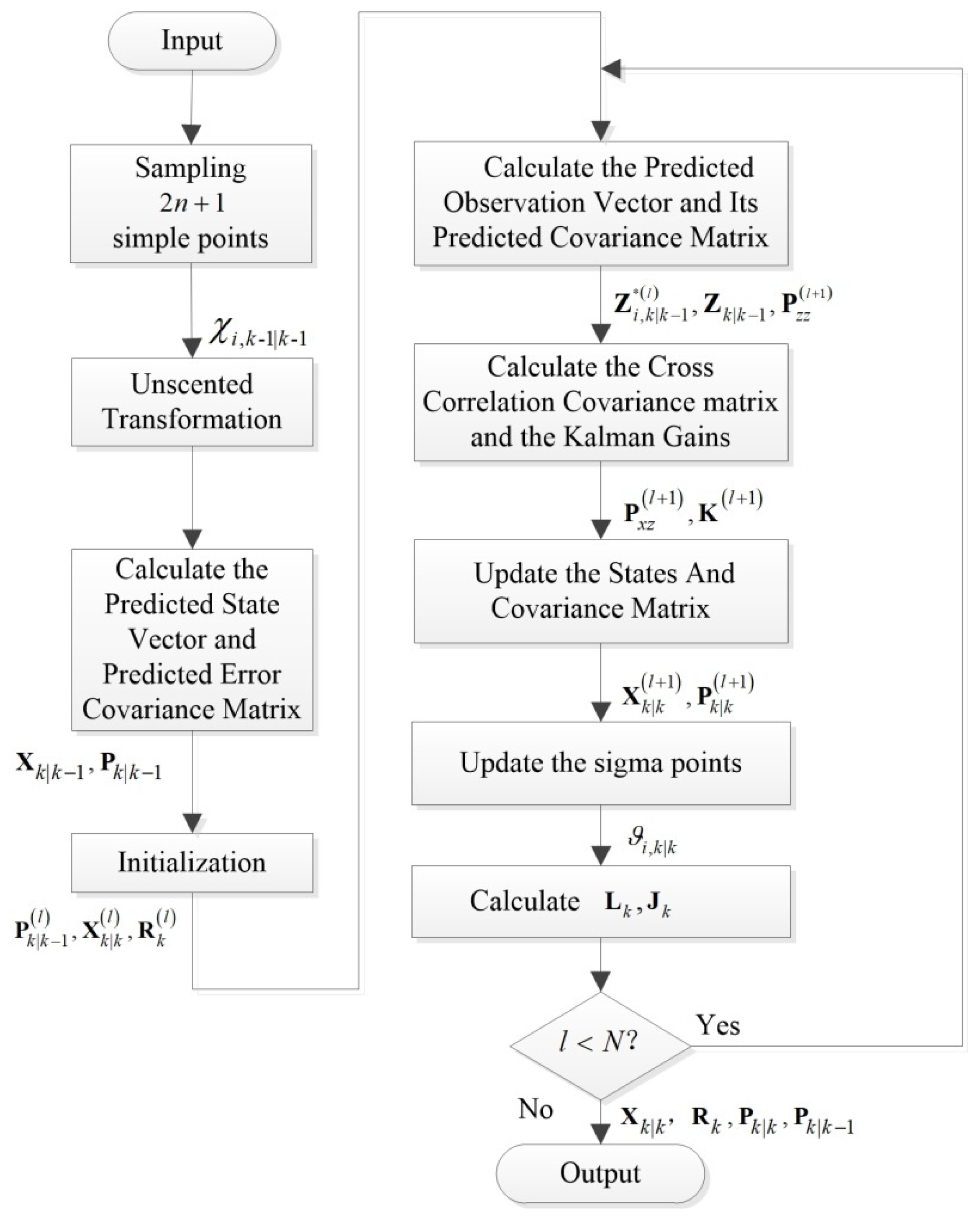
Figure 4 shows the flowchart of the proposed SRAKF. First, the nine-axis sensor processed data are calculated to obtain the measurements. Subsequently, $X_{k|k-1}$ and $P_{k|k-1}$ are computed by the process of time update according to Equations (13)–(15). $X_{k|k-1}$ and $P_{k|k-1}$ are calculated as the initial value of the expectation maximization method iteration. After iteration $N$, the accurate $R_k$ and $P_{k|k-1}$ at time $k$ are acquired. $R_k$ is renewed by Equation (27). $P_{k|k-1}$ is updated by Equation (28) because the state formula is nonlinear. Values of $X_{k|k}$ and $P_{k|k}$ with higher accuracy at time $k$ have not been obtained.

3.3. The Analysis of the Convergence of the Proposed Algorithm

Remark 4:

$X_{k|k-1}$ is derived from ${\chi }_{i,k-1|k-1}$, which is calculated according to $P_{k|k}$. $P_{k|k}$ is derived from $P_{k|k-1}$ and $R_k$. Hence, both $P_{k|k-1}$ and $R_k$ have a direct influence on the iterative formula. Therefore, the EM approach is employed to calculate the $P_{k|k-1}$ and $R_k$ online.

Proof: 

Calculate the estimations of $P_{k|k-1}$ and $R_k$ based on $Z_{1:k}$, where $Z_{1:k}$ includes all of the measurement information from time 1 to $k$, and the MLE is selected to infer $P_{k|k-1}$ and $R_k$ because the MLE has asymptotic efficiency and strong consistency. □

However, it is impossible to obtain $\log p_{{\mathsf{\Phi }}_k}(X_{k|k},Z_{1:k})$ because $X_{k|k}$ is unobserved at time $k$. Using Equation (10), the suboptimal solution of ${\mathsf{\Phi }}_k$ at the number of the $l+1$th iteration can be transformed into the subsequent suboptimal problem. It is defined that ${\mathsf{\Phi }}_k^{\left(l+1\right)}$ denotes an approximate solution of ${\widehat{\mathsf{\Phi }}}_k$ at the $l+1$th iteration, and it can be approximated as:

$${\mathsf{\Phi }}_k^{\left(l+1\right)}\approx \arg \underset{{\mathsf{\Phi }}_k}{\max }\mathsf{\Omega }({\mathsf{\Phi }}_k,{\mathsf{\Phi }}_k^{\left(l\right)})$$

(34)

Employing the Bayesian theory, Equation (10) could be given by Equation (35):

$$\begin{array}{c}\mathsf{\Omega }({\mathsf{\Phi }}_k,{\mathsf{\Phi }}_k^{\left(l\right)})={\displaystyle \int [\log p_{{\mathsf{\Phi }}_k}(X_{k|k}|Z_{1:k})p_{{\mathsf{\Phi }}_k}(Z_{1:k})]}{p}_{{\mathsf{\Phi }}_k^{\left(l\right)}}(X_{k|k}|Z_{1:k})d{X}_{k|k}\\ \hspace{1em}\hspace{1em}\hspace{1em}\hspace{1em}\hspace{1em}\hspace{1em} ={\displaystyle \int [\log p_{{\mathsf{\Phi }}_k}(X_{k|k}|Z_{1:k})+\log p_{{\mathsf{\Phi }}_k}(Z_{1:k})]}{p}_{{\mathsf{\Phi }}_k^{\left(l\right)}}(X_{k|k}|Z_{1:k})d{X}_{k|k}\\ \hspace{1em}\hspace{1em}\hspace{1em}\hspace{1em}\hspace{1em}\hspace{1em}={\displaystyle \int \log p_{{\mathsf{\Phi }}_k}(X_{k|k}|Z_{1:k})}{p}_{{\mathsf{\Phi }}_k^{\left(l\right)}}(X_{k|k}|Z_{1:k})d{X}_{k|k}+\log p_{{\mathsf{\Phi }}_k}(Z_{1:k})\end{array}$$

(35)

Making use of ${\mathsf{\Phi }}_k={\mathsf{\Phi }}_k^{\left(l\right)}$ in Equation (35), we derive

$$\partial \mathsf{\Omega }\left({\mathsf{\Phi }}_k^{\left(l\right)},{\mathsf{\Phi }}_k^{\left(l\right)}\right)={\displaystyle \int \log p_{{\mathsf{\Phi }}_k^{\left(l\right)}}\left(X_{k|k}|Z_{1:k}\right)p_{{\mathsf{\Phi }}_k^{\left(l\right)}}\left(X_{k|k}|Z_{1:k}\right)d{X}_{k|k}}+\log p_{{\mathsf{\Phi }}_k^{\left(l\right)}}\left(Z_{1:k}\right)$$

(36)

Subtracting Equation (36) from Equation (35), the following equation is derived:

$$\begin{array}{l}\log p_{{\mathsf{\Phi }}_k}(Z_{1:k})-\log p_{{\mathsf{\Phi }}_k^{\left(l\right)}}(Z_{1:k})=\\ KLD\left(p_{{\mathsf{\Phi }}_k^{\left(l\right)}}(X_{k|k}|Z_{1:k})||p_{{\mathsf{\Phi }}_k}(X_{k|k}|Z_{1:k})\right)+\mathsf{\Omega }({\mathsf{\Phi }}_k,{\mathsf{\Phi }}_k^{\left(l\right)})-\mathsf{\Omega }({\mathsf{\Phi }}_k^{\left(l\right)},{\mathsf{\Phi }}_k^{\left(l\right)})\end{array}$$

(37)

where the Kullback–Leibler divergence defined in Equation (38) is considered nonnegative, then the following equation is derived:

$$KLD\left(p_{{\mathsf{\Phi }}_k^{\left(l\right)}}(X_{k|k}|Z_{1:k})||p_{{\mathsf{\Phi }}_k}(X_{k|k}|Z_{1:k})\right)=[{\displaystyle \int p_{{\mathsf{\Phi }}_k^{\left(l\right)}}(X_{k|k}|Z_{1:k})}\log \left[\frac{p_{{\mathsf{\Phi }}_k^{\left(l\right)}}(X_{k|k}|Z_{1:k})}{p_{{\mathsf{\Phi }}_k}(X_{k|k}|Z_{1:k})}\right]d{X}_{k|k}]$$

(38)

Using Equation (38), it can be calculated that

$$\mathsf{\Omega }({\mathsf{\Phi }}_k^{\left(l\right)},{\mathsf{\Phi }}_k^{\left(l\right)})-\mathsf{\Omega }({\mathsf{\Phi }}_k,{\mathsf{\Phi }}_k^{\left(l\right)})\ge \log p_{{\mathsf{\Phi }}_k^{\left(l\right)}}(Z_{1:k})-\log p_{{\mathsf{\Phi }}_k}(Z_{1:k})$$

(39)

Therefore, one can see from Equation (39) that choosing ${\mathsf{\Phi }}_k^{\left(l+1\right)}$ can guarantee that $\log p_{{\mathsf{\Phi }}_k}(Z_{1:k})$ is not reduced in the process of each iteration. When $l\to +\infty$, the maximum solution of $\mathsf{\Omega }({\mathsf{\Phi }}_k,{\mathsf{\Phi }}_k^{\left(l\right)})$ can be regarded as an approximate maximum solution of $\log p_{{\mathsf{\Phi }}_k}(Z_{1:k})$. If a suitable ${\mathsf{\Phi }}_k$ is selected, ${\mathsf{\Phi }}_k^{\left(l\right)}$ will be convergent to the MLE based on this good property of the EM approach. ${\mathsf{\Phi }}_k^{\left(l\right)}$ equaling ${\widehat{\mathsf{\Phi }}}_k$ ensures the local convergence of each iteration.

4. Lake Trial Experiments and Results

4.1. The Accuracy Verification of the SRAKF

Many types of interference, such as magnetic interference, will inevitably lead to INS errors in a marine environment. Hence, the positions determined by navigation system may be inaccurate. The effectiveness and performance of the SRAKF are verified by employing post-processed data gathered in lake experiments. The lake used in the trials is a freshwater lake, and the temperature of the lake is less than 20 °C, and the salinity and temperature have no influence on positioning information estimated by the IMU. The non-Gaussian noises $v_{non}$ are added in the measurement vector to simulate the complex underwater environment, and the noise model is shown as Equation (40).

$$Z=HX+v+v_{non}$$

(40)

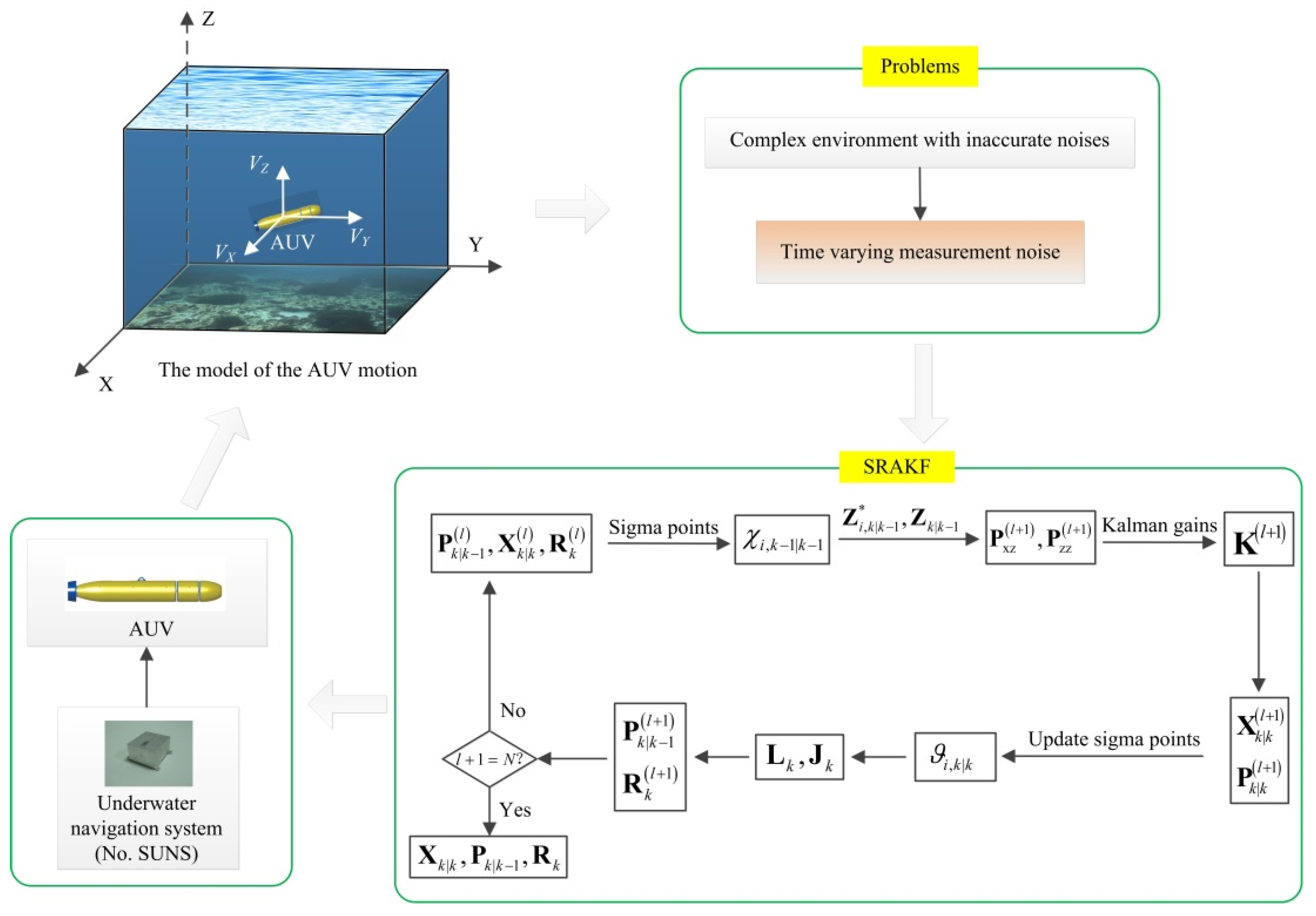
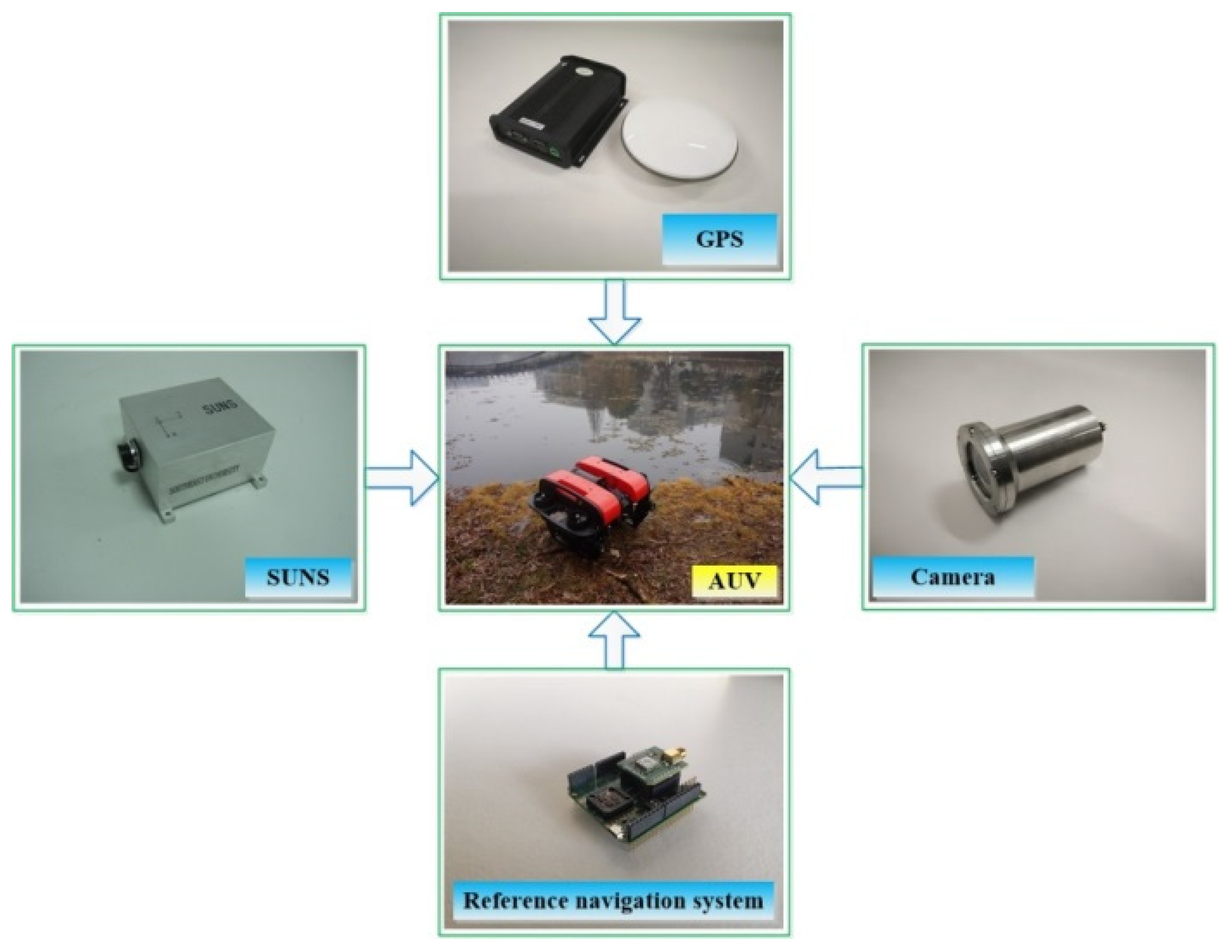
The navigation information is acquired by SUNS (designed by our lab) during the process of a vehicle diving into the water. The high-precision inertial navigation system is chosen as the reference. When the vehicle comes to the surface of the water, the position information is updated by the GPS. The structure of the algorithm verification in the underwater experiment platform is denoted in Figure 5, and the platform of the underwater positioning trial is presented in Figure 6. ADIS16xx was used as the IMU, and its specifications are shown in

Table 2. The specifications for IMU.

Accelerometers	Resolution	0.1 mg(at ± 2 g range)
	Bias in-run stability (RMS, Allan variance)	50 μg
	SF accuracy	0.1%
Gyroscopes	Resolution	0.01 deg/sec (at ± 250 deg/sec range)
	Bias in-run stability (RMS, Allan variance)	4 deg/hr
	SF accuracy	0.01%
Magnetometers	Resolution	10 nT
	Bias in-run stability (RMS, Allan variance)	0.1 nT
	SF accuracy	0.02%

. The underwater vehicle obtained a lot of raw data in the lake trial. With the proposed SRAKF, the data are processed and analyzed soon afterwards, compared to the traditional UKF and CKF. ${\mathrm{RMSE}}_{\mathrm{La}}$ and ${\mathrm{RMSE}}_{\mathrm{Lo}}$ denote the RMSE of the latitude and longitude, respectively.

4.1.1. Case 1: Surface Lake Trial

The AUV’s positions can be renewed by the GPS for a period of time while refloating. When the GPS signal is blocked, the accuracy of the integrated navigation system will be extremely poor or even inaccurate. SRAKF performance is evaluated in the surface trial.

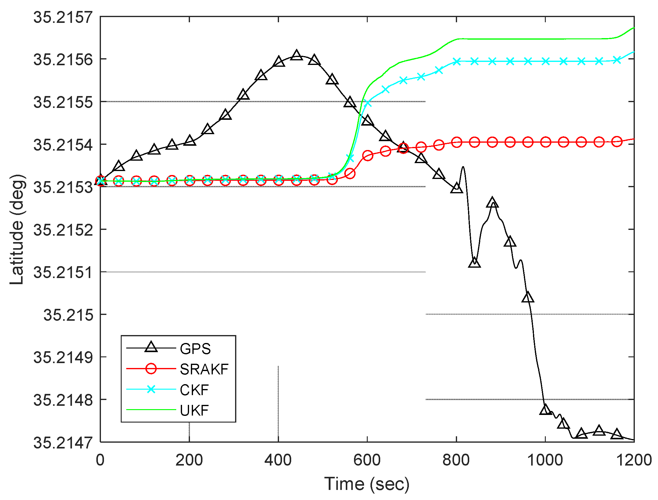
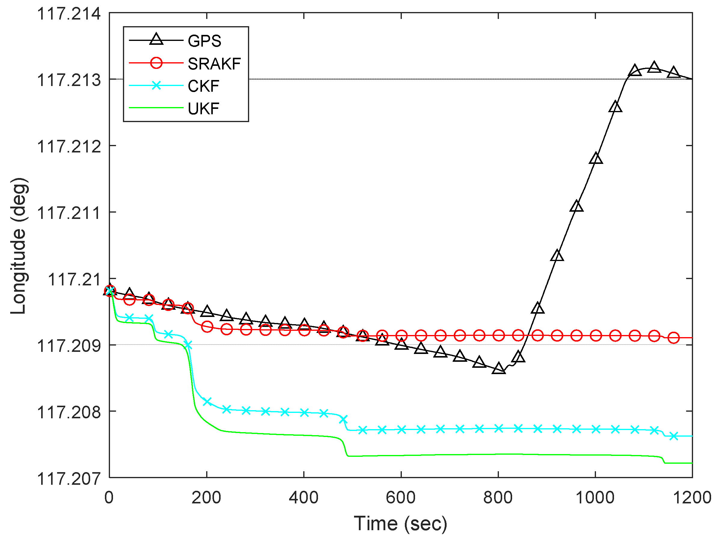
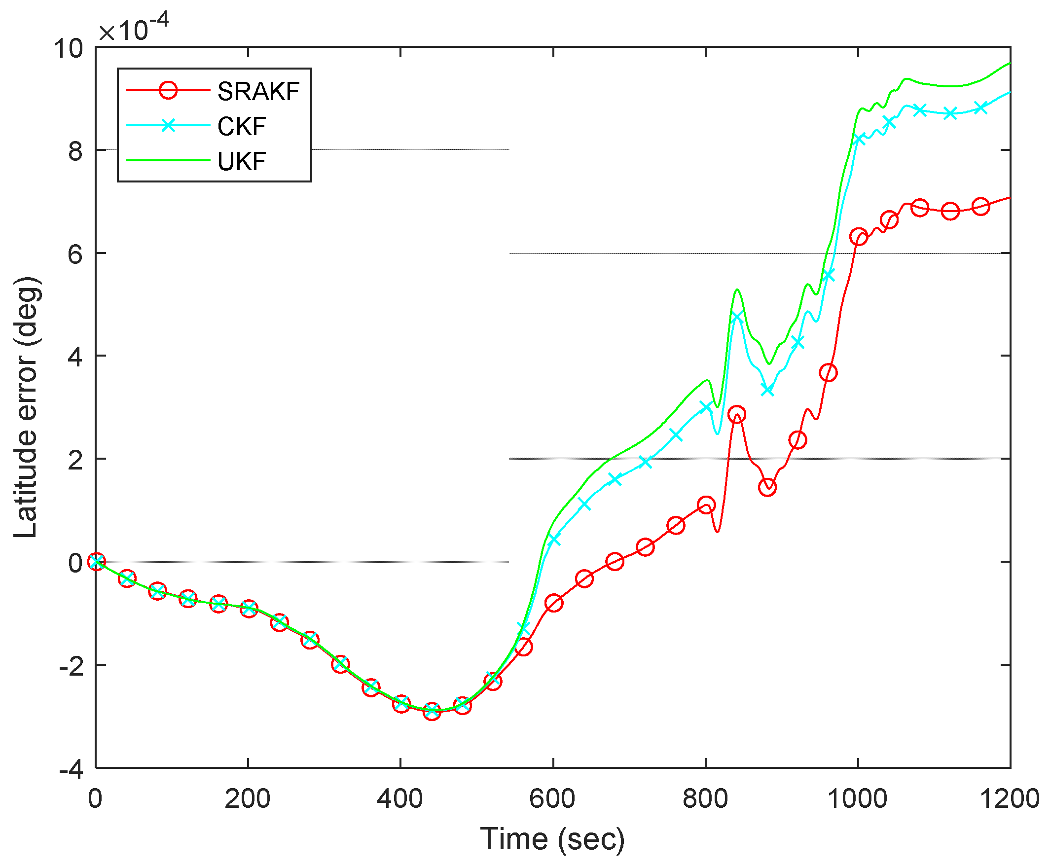
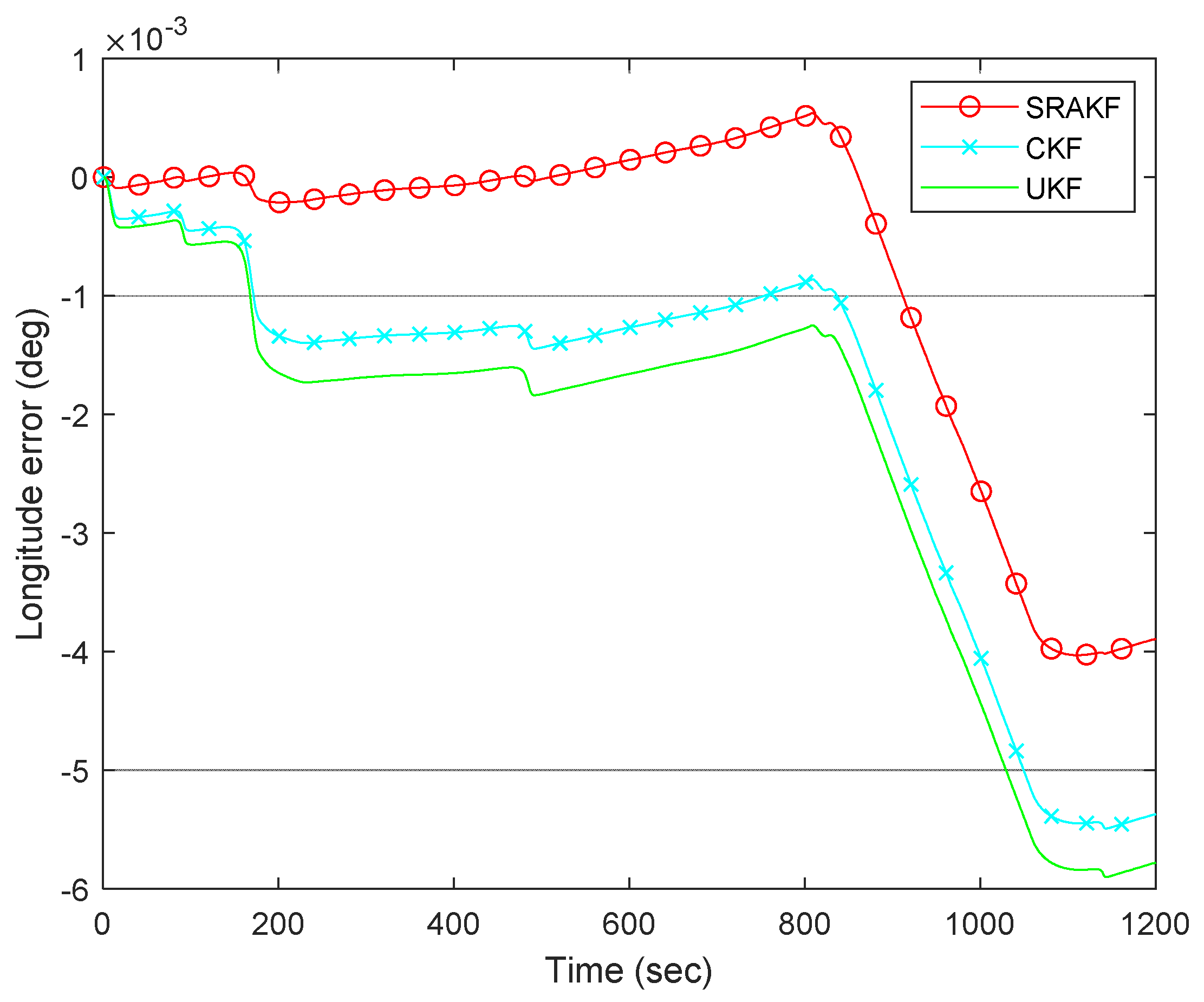
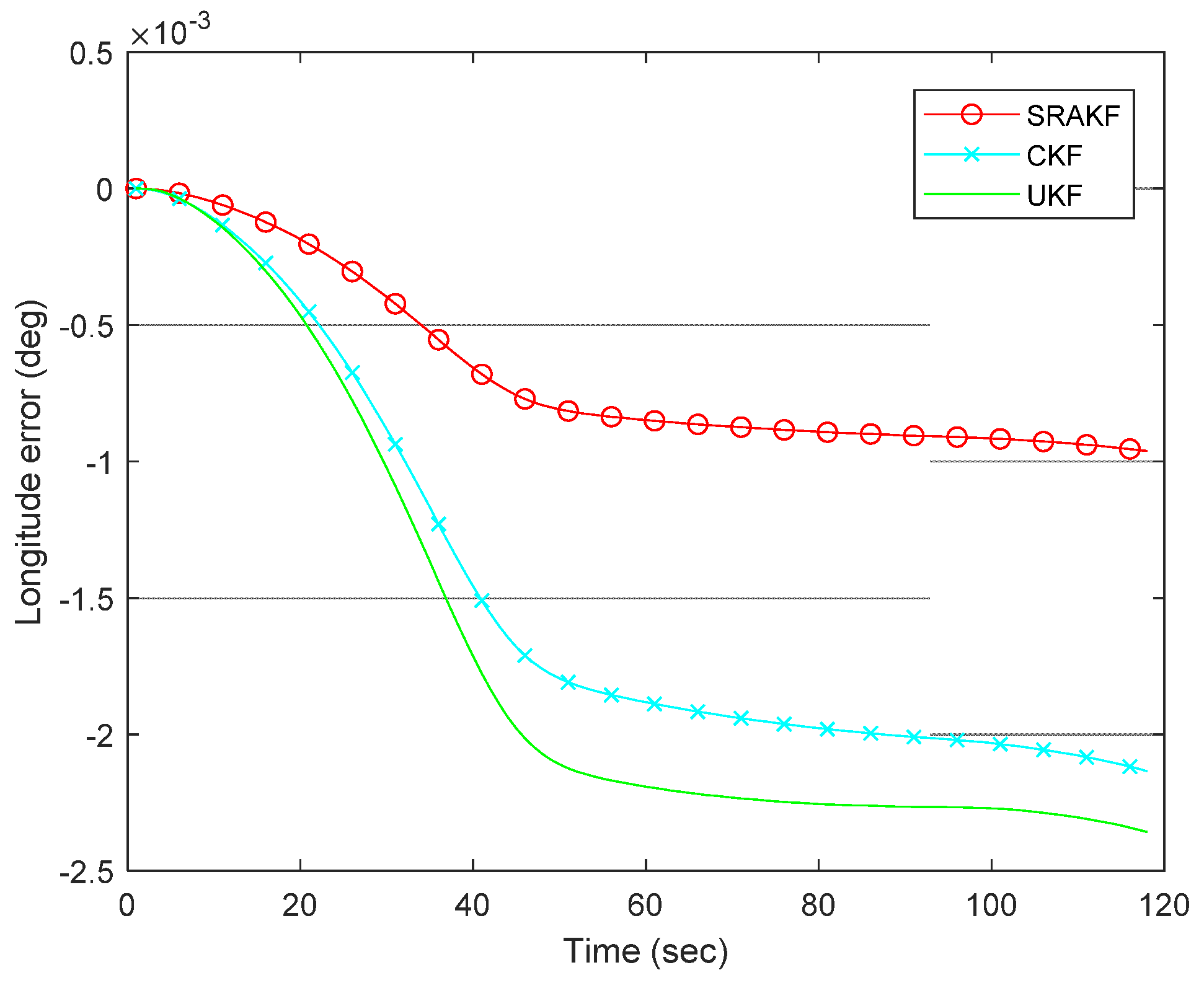
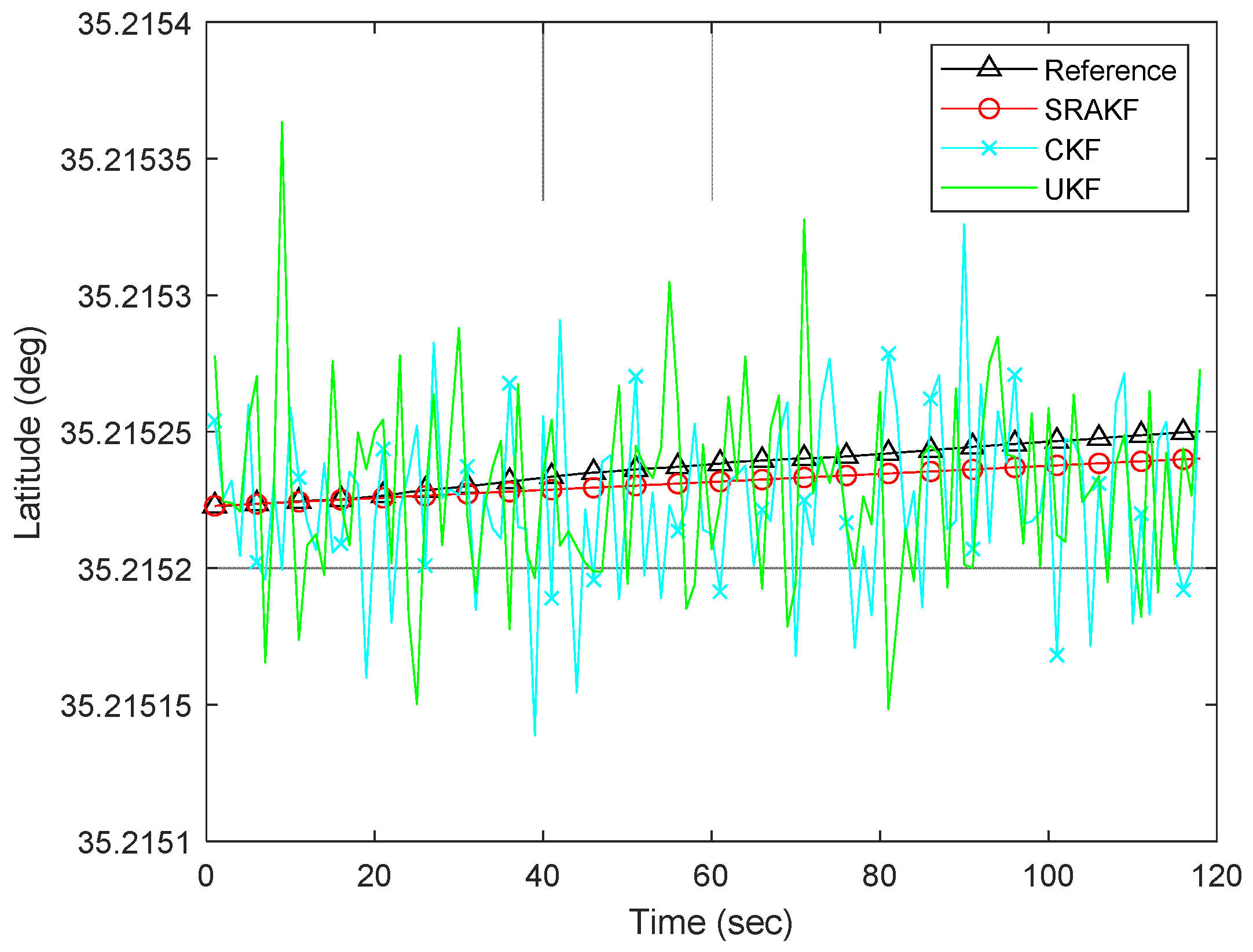
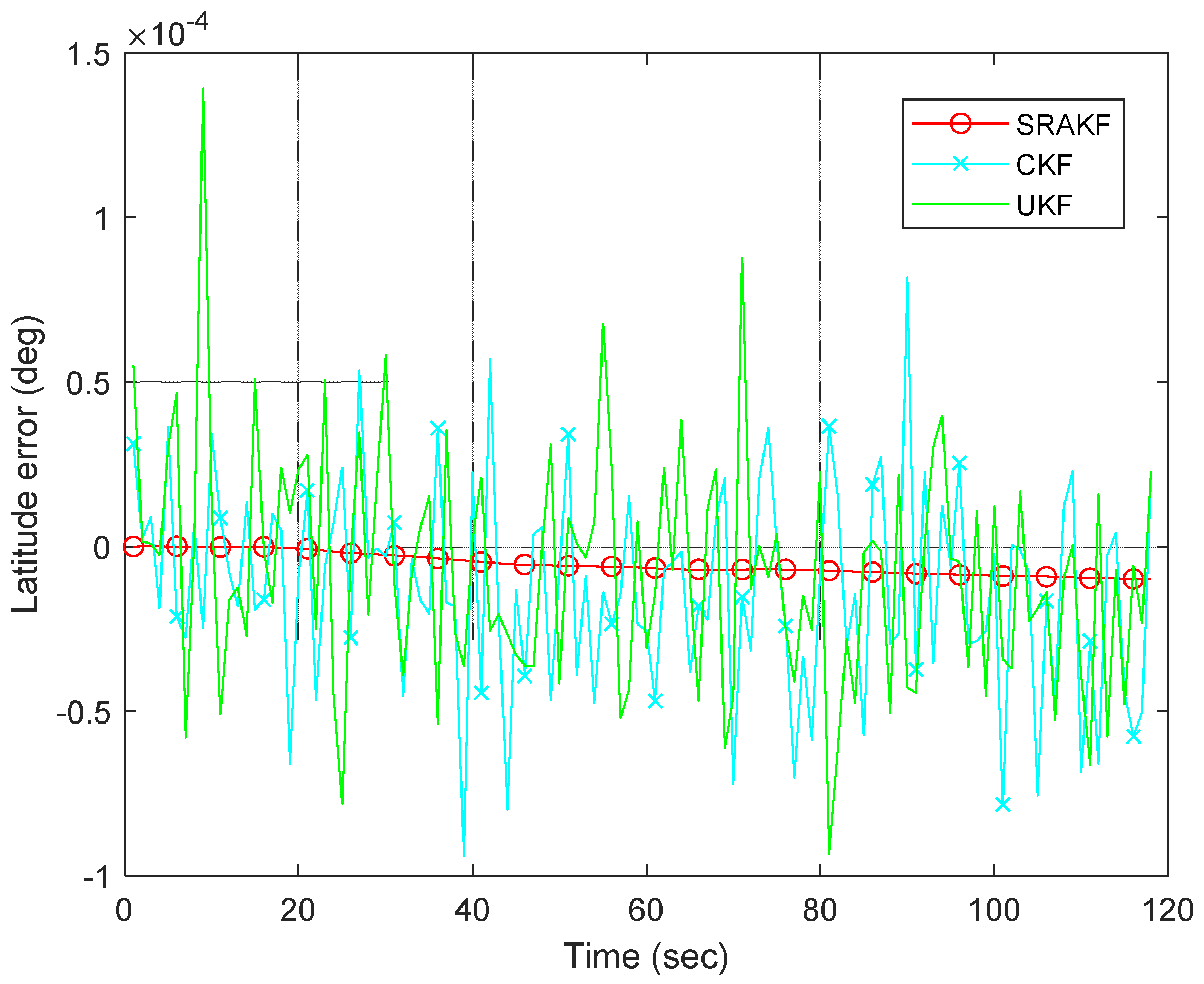
In Case 1, Figure 7 and Figure 8 show the trajectory comparison results between the SRAKF and other traditional algorithms. The position (latitude and longitude) errors are shown in Figure 9 and Figure 10, respectively. Furthermore, the RMSE of position for SRAKF, UKF, and CKF are shown in

Table 3. RMSE for different algorithms.

	Algorithms	UKF	CKF	SRAKF
RMSE
${\mathrm{RMSE}}_{\mathrm{La}}$(deg)		3.4998 × 10−4	3.2523 × 10−4	2.4298 × 10−4
${\mathrm{RMSE}}_{\mathrm{Lo}}$(deg)		2.2862 × 10−3	1.9509 × 10−3	8.9344 × 10−4

.

From Figure 7 and Figure 8, it can be clearly seen that the performance of the proposed SRAKF is much better than UKF and CKF. In Table 3, we can see that by employing the proposed SRAKF, the ${\mathrm{RMSE}}_{\mathrm{La}}$ is reduced from 3.4998 × 10⁻⁴ deg to 2.4298 × 10⁻⁴ deg. The ${\mathrm{RMSE}}_{\mathrm{Lo}}$ for SRAKF is 8.9344 × 10⁻⁴ deg, which is the lowest of the three algorithms.

4.1.2. Case 2: Underwater Lake Trial

In Case 2, the trajectory comparison results for SRAKF, UKF, and CKF are shown in Figure 11 and Figure 12. The latitude and longitude errors are shown in Figure 13 and Figure 14, respectively. The RMSE of position for SRAKF, UKF, and CKF are shown in

Table 4. RMSE for different algorithms.

	Algorithms	UKF	CKF	SRAKF
RMSE
${\mathrm{RMSE}}_{\mathrm{La}}$(deg)		1.1179 × 10−5	4.6089 × 10−6	2.0964 × 10−6
${\mathrm{RMSE}}_{\mathrm{Lo}}$ (deg)		1.6797 × 10−3	1.4708 × 10−3	6.6276 × 10−4

.

From Figure 11 and Figure 12, it can be concluded that the estimation accuracy in terms of the position for SRAKF is superior to that of UKF and CKF. In Table 4, by employing the proposed SRAKF, the ${\mathrm{RMSE}}_{\mathrm{La}}$ for SRAKF is 2.0964 × 10⁻⁶ deg, which is lower than UKF and CKF. In Figure 14, the SRAKF method has the lowest longitude errors and the ${\mathrm{RMSE}}_{\mathrm{Lo}}$ for SRAKF is 6.6276 × 10⁻⁴ deg, which is the lowest compared to UKF and CKF.

From the experimental results, it is obvious that the proposed algorithm is superior to other algorithms. The errors change continuously along with time during positioning. The bigger errors are caused if measurement errors are not updated in real time. The one-step predicted covariance becomes inaccurate due to measurement errors. It is essential to update both the measurement error and the one-step predicted covariance. However, the UKF and CKF errors mainly include two factors: sigma points and the measurement errors are not updated in real time. The truncation errors are likely eliminated since the localization linearization is not used in the proposed SRAKF. Moreover, the real-time update is performed for the measurement error and one-step predicted covariance by employing SRAKF. SRAKF has the best performance in terms of of state estimation.

When the sensors loaded in the AUV are affected by larger noises, SRAKF can still make an adjustment for $P_{k|k-1}$ and $R_k$ adaptively. Hence, accurate information for $P_{k|k-1}$ and $R_k$ can make the algorithm more stable. However, UKF and CKF cannot deal with larger noise because the large noise measurement has a great impact on calculating $P_{zz}$ and $P_{\mathrm{xz}}$. $P_{zz}$ and $P_{\mathrm{xz}}$ also influence the Kalman gain. SRAKF performs better than UKF and CKF because it can estimate the optimal solutions of $P_{k|k-1}$ and $R_k$ in each EM iteration. Meanwhile, $X_{k|k}$ and $P_{k|k}$ are updated by using the accurate $P_{k|k-1}$ and $R_k$, so the accuracy and the robustness of SRAKF are greatly improved.

4.2. The Robustness Lake Trial

The noise measurement is enlarged to verify SRAKF’s robustness. At the time k, the noise measurement is chosen to be one time and two times as much as the reference value of the noise measurement.

$${\overline{R}}_k=\{\begin{array}{cc}{R}_k& {\mathrm{P}}_r[0,0.95]\\ 2R_k& {\mathrm{P}}_o[0.95,1]\end{array}$$

(41)

where ${\mathrm{P}}_r$ and ${\mathrm{P}}_o$ are the probabilities of the reference value the noise measurement and outlier, respectively; where [0,0.95] denotes the reference value of the noise measurement, and [0.95,1] denotes the outlier at time $k$, respectively.

In the robustness lake trial, the trajectory comparison results for SRAKF, UKF, and CKF are shown in Figure 15 and Figure 16. The latitude and longitude errors are shown in Figure 17 and Figure 18, respectively. To obtain the quantization results, the RMSE of the position for SRAKF, UKF, and CKF are shown in

Table 5. RMSE for different algorithms.

	Algorithms	UKF	CKF	SRAKF
RMSE
${\mathrm{RMSE}}_{\mathrm{La}}$(deg)		2.9388 × 10−5	2.9013 × 10−5	5.4470 × 10−6
${\mathrm{RMSE}}_{\mathrm{Lo}}$(deg)		2.3801 × 10−3	2.3713 × 10−3	1.4696 × 10−4

.

From Figure 17 and Figure 18, it can be concluded that the estimation accuracy in terms of positions for SRAKF is superior to that of UKF and CKF. In order to further compare the performance of the three algorithms, the results of error analysis are also shown in Table 5. In Table 5, the SRAKF latitude error is less than the other two algorithms, where the former ${\mathrm{RMSE}}_{\mathrm{La}}$ is 5.4470 × 10⁻⁶ deg, and the UKF and CKF are 2.9388 × 10⁻⁵ deg and 2.9013 × 10⁻⁵ deg, respectively. The improvement in ${\mathrm{RMSE}}_{\mathrm{La}}$ is about 81.47% and 81.23% compared to UKF and CKF, respectively. In Figure 18, by employing the proposed SRAKF, the ${\mathrm{RMSE}}_{\mathrm{Lo}}$ for SRAKF is 1.4696 × 10⁻⁴ deg, which is lower than UKF and CKF. SRAKF reduces the ${\mathrm{RMSE}}_{\mathrm{Lo}}$ by about 93.83% and 93.80% compared to UKF and CKF, respectively, so the position estimation accuracy has greatly been improved by the proposed SRAKF.

It can be seen that SRAKF performs better than UKF and CKF in handling with the changeable measurement noises. When the sensors are influenced by large noise, the SRAKF can still adaptively make an adjustment for $R_k$ and $P_{k|k-1}$, and it can make the algorithm more stable during the whole trial. However, the UKF cannot deal with the larger noise, because the large noise has a great impact on $X_{k|k-1}$ and $P_{k|k-1}$. In other words, SRAKF outperforms UKF and CKF because it can estimate $P_{k|k-1}$ and $R_k$ by using the EM method to choose the suboptimal solution of ${\mathsf{\Phi }}_k$. Meanwhile, the truncation errors are effectively eliminated by the unscented transformation, so the estimation accuracy of the algorithm is improved greatly. Hence, the proposed SRAKF has best performance among three algorithms when the noise measurement is time-varying.

5. Conclusions

The unknown and changeable underwater environment inevitably makes accurate positioning hard for MEMS-grade INS carried in AUV. It is difficult for traditional algorithms to obtain state information. The performance of the proposed SRAKF is deduced theoretically and tested through lake trials. The experiment results demonstrate that the SRAKF can calculate the position of AUVs more accurately than the other two traditional algorithms, even if the noise measurements are enlarged and changeable. The position of the AUV can be obtained with higher accuracy using the proposed SRAKF algorithm. Moreover, not only are accuracy and efficiency achieved by the SRAKF, but the SRAKF has better robustness in terms of position estimation.

References

1. Walker, C.R.; Stringfield, J.Q.; Wolbrecht, E.T.; Anderson, M.J.; Canning, J.R.; Bean, T.A.; Odell, D.L.; Frenzel, J.F.; Edwards, D.B. Measurement of the Magnetic Signature of a Moving Surface Vessel with Multiple Magnetometer-Equipped AUVs. Ocean Eng. 2013, 64, 80–87. [Google Scholar] [CrossRef]
2. Eriksen, C.C.; Osse, T.J.; Light, R.D.; Wen, T.; Lehman, T.W.; Sabin, P.L.; Ballard, J.W.; Chiodi, A.M. Seaglider: A Long-Range Autonomous Underwater Vehicle for Oceanographic Research. IEEE J. Ocean. Eng. 2001, 26, 424–436. [Google Scholar] [CrossRef] [Green Version]
3. Qin, J.H.; Wang, S.; Kang, Y.; Liu, Q.C. Circular Formation Algorithms for Multiple Nonholonomic Mobile Robots: An Optimization-based Approach. IEEE Trans. Ind. Electron. 2019, 66, 3693–3701. [Google Scholar] [CrossRef]
4. Stutters, L.; Liu, H.H.; Tiltman, C.; Brown, D.J. Navigation Technologies for Autonomous Underwater Vehicles. IEEE Trans. Syst. Man Cybern. Part C Appl. Rev. 2008, 38, 581–589. [Google Scholar] [CrossRef]
5. Grenon, G.; An, P.E.; Smith, S.M.; Healey, A.J. Enhancement of the Inertial Navigation System for the Morpheus Autonomous Underwater Vehicles. IEEE J. Ocean. Eng. 2001, 26, 548–560. [Google Scholar] [CrossRef]
6. Morton, R.A.; Leach, M.P.; Paine, J.G.; Cardoza, M.A. Monitoring Beach Changes Using GPS Surveying Techniques. J. Coast. Res. 1993, 9, 702–720. [Google Scholar]
7. Watson, C.; Coleman, R.; Handsworth, R. Coastal Tide Gauge Calibration: A Case Study at Macquarie Island Using GPS Buoy Techniques. J. Coast. Res. 2008, 24, 1071–1079. [Google Scholar] [CrossRef]
8. Crassidis, J.L.; Lai, K.L.; Harman, R.R. Real-Time Attitude-Independent Three-Axis Magnetometer Calibration. J. Guid. Control Dyn. 2005, 28, 114–117. [Google Scholar] [CrossRef]
9. Xiong, K.; Liu, L.; Liu, Y. Non-Linear Robust Filter Design for Satellite Attitude Determination. IET Control Theory Appl. 2010, 4, 1222–1234. [Google Scholar] [CrossRef]
10. Nemra, A.; Aouf, N. Robust INS/GPS Sensor Fusion for UAV Localization Using SDRE Nonlinear Filtering. IEEE Sens. J. 2010, 10, 789–798. [Google Scholar] [CrossRef] [Green Version]
11. Yao, Q.J. Adaptive Finite-Time Sliding Mode Control Design for Finite-Time Fault-Tolerant Trajectory Tracking of Marine Vehicles with Input Saturation. J. Frankl. Inst. Eng. Appl. Math. 2020, 357, 13593–13619. [Google Scholar] [CrossRef]
12. Huang, H.Q.; Shi, R.D.; Zhou, J.; Yang, Y.; Song, R.; Chen, J.F.; Wu, G.Q.; Zhang, J.J. Attitude Determination Method Integrating Square-Root Cubature Kalman Filter with Expectation-Maximization for Inertial Navigation System Applied to Underwater Glider. Rev. Sci. Instrum. 2019, 90, 095001. [Google Scholar] [CrossRef] [PubMed] [Green Version]
13. Wang, Y.; Zhang, H.; Xu, L.W.; Cao, C.H.; Gulliver, T.A. Adoption of Hybrid Time Series Neural Network in the Underwater Acoustic Signal Modulation Identification. J. Frankl. Inst. Eng. Appl. Math. 2020, 357, 13906–13922. [Google Scholar] [CrossRef]
14. Wang, Y.Y.; Hu, J.B. Robust Control for a Quadrotor Aircraft with Small Overshoot and High-Precision Position Tracking Performance. J. Frankl. Inst. Eng. Appl. Math. 2020, 357, 13386–13409. [Google Scholar] [CrossRef]
15. Loebis, D.; Sutton, R.; Chudley, J.; Naeem, W. Adaptive Tuning of a Kalman Filter via Fuzzy Logic for an Intelligent AUV Navigation System. Control Eng. Pract. 2004, 12, 1531–1539. [Google Scholar] [CrossRef]
16. Dong, L.Y.; Xu, H.L.; Feng, X.S.; Han, X.J.; Yu, C. An Adaptive Target Tracking Algorithm Based on EKF for AUV with Unknown Non-Gaussian Process Noise. Appl. Sci. 2020, 10, 3413. [Google Scholar] [CrossRef]
17. Noureldin, A.; Karamat, T.B.; Eberts, M.D.; El-Shafie, A. Performance Enhancement of MEMS-Based INS/GPS Integration for Low-Cost Navigation Applications. IEEE Trans. Veh. Technol. 2009, 58, 1077–1096. [Google Scholar] [CrossRef]
18. Huang, H.Q.; Chen, X.Y.; Zhang, B.; Wang, J. High Accuracy Navigation Information Estimation for Inertial System Using the Multi-Model EKF Fusing Adams Explicit Formula Applied to Underwater Gliders. ISA Trans. 2017, 66, 414–424. [Google Scholar] [CrossRef]
19. Li, W.L.; Wu, W.Q.; Wang, J.L.; Lu, L.Q. A Fast SINS Initial Alignment Scheme for Underwater Vehicle Applications. J. Navig. 2013, 66, 181–198. [Google Scholar] [CrossRef] [Green Version]
20. Julier, S.; Uhlmann, J.; Durrant-Whyte, H.F. A New Method for the Nonlinear Transformation of Means and Covariances in Filters and Estimators. IEEE Trans. Autom. Control 2000, 45, 477–482. [Google Scholar] [CrossRef] [Green Version]
21. Zhou, H.; Zhao, H.; Huang, H.Q.; Zhao, X. A Cubature-Principle-Assisted IMM-Adaptive UKF Algorithm for Maneuvering Target Tracking Caused by Sensor Faults. Appl. Sci. 2017, 7, 1003. [Google Scholar] [CrossRef] [Green Version]
22. Huang, Y.L.; Zhang, Y.G.; Chambers, J.A. A Novel Kullback–Leibler Divergence Minimization-Based Adaptive Student’s t-Filter. IEEE Trans. Signal Process. 2019, 67, 5417–5432. [Google Scholar] [CrossRef]
23. Tong, X.; Su, Y.; Li, Z.F.; Si, C.W.; Han, G.W.; Ning, J.; Yang, F.H. A Double-Step Unscented Kalman Filter and HMM-Based Zero-Velocity Update for Pedestrian Dead Reckoning Using MEMS Sensors. IEEE Trans. Ind. Electron. 2020, 67, 581–591. [Google Scholar] [CrossRef]
24. Chen, Y.; Lee, M.K.; Birla, M.B.; Li, H.J.; Li, G.M.; Duan, X.Y.; Wang, T.D.; Oldham, K.R. Motion Estimation for a Compact Electrostatic Microscanner via Shared Driving and Sensing Electrodes in Endomicroscopy. IEEE/ASME Trans. Mechatron. 2020, 25, 661–672. [Google Scholar] [CrossRef]
25. Huang, H.Q.; Tang, J.C.; Zhang, B.; Chen, J.F.; Zhang, J.J.; Song, X. A Novel Nonlinear Algorithm for Non-Gaussian Noises and Measurement Information Loss in Underwater Navigation. IEEE Access 2020, 8, 118472–118484. [Google Scholar] [CrossRef]
26. Cao, H.L.; Zhang, Y.J.; Han, Z.Q.; Shao, X.L.; Gao, J.Y.; Huang, K.; Shi, Y.B.; Tang, J.; Shen, C.; Liu, J. Pole-Zero-Temperature Compensation Circuit Design and Experiment for Dual-Mass MEMS Gyroscope Bandwidth Expansion. IEEE/ASME Trans. Mechatron. 2019, 24, 677–688. [Google Scholar] [CrossRef]
27. Zhu, Y.X.; Cheng, X.H.; Hu, J.; Zhou, L.; Fu, J.B. A Novel Hybrid Approach to Deal with DVL Malfunctions for Underwater Integrated Navigation Systems. Appl. Sci. 2017, 7, 759. [Google Scholar] [CrossRef] [Green Version]
28. Moon, T.K. The Expectation-Maximization Algorithm. IEEE Signal Process. Mag. 1996, 13, 47–60. [Google Scholar] [CrossRef]
29. Gu, Y.; Liu, J.C.; Li, X.L.; Chou, Y.X.; Ji, Y. State Space Model Identification of Multirate Processes with Time-Delay Using the Expectation Maximization. J. Frankl. Inst. Eng. Appl. Math. 2019, 356, 1623–1639. [Google Scholar] [CrossRef]
30. Huang, H.Q.; Tang, J.C.; Liu, C.; Zhang, B.; Wang, B. Variational Bayesian-Based Filter for Inaccurate Input in Underwater Navigation. IEEE Trans. Veh. Technol. 2021. [Google Scholar] [CrossRef]
31. Huang, H.Q.; Chen, X.Y.; Zhou, Z.K.; Liu, H.; Lv, C.P. Study on INS/DR Integration Navigation System Using EKF/RK4 Algorithm for Underwater Gliders. J. Mar. Sci. Technol. 2017, 25, 84–95. [Google Scholar]
32. Huang, H.Q.; Zhou, J.; Zhang, J.; Yang, Y.; Song, R.; Chen, J.F.; Zhang, J.J. Attitude Estimation Fusing Quasi-Newton and Cubature Kalman Filtering for Inertial Navigation System Aided with Magnetic Sensors. IEEE Access 2018, 6, 28755–28767. [Google Scholar] [CrossRef]
33. Ghahramani, Z. Learning Dynamic Bayesian Network, Adaptive Processing of Temporal Information, Lecture Notes in Artificial Intelligence; Springer: Berlin/Heidelberg, Germany, 1997. [Google Scholar]
34. Bar-Shalom, Y.; Li, X.R.; Kirubarajan, T. Estimation with Applications to Tracking and Navigation; Wiley: New York, NY, USA, 2001. [Google Scholar]
35. Lefebvre, T.; Bruyninckx, H.; De Schutter, J. Comment on “A New Method for the Nonlinear Transformation of Means and Covariances in Filters and Estimators”. IEEE Trans. Autom. Control 2001, 47, 1406–1408. [Google Scholar] [CrossRef] [Green Version]
36. Schön, T.B.; Wills, A.; Ninness, B. System Identification of Nonlinear State-Space Models. Automatica 2011, 47, 39–49. [Google Scholar] [CrossRef] [Green Version]
37. Zhao, S.Y.; Liu, F. Bayesian Estimation for Jump Markov Linear Systems with Non-Homogeneous Transition Probabilities. J. Frankl. Inst. Eng. Appl. Math. 2013, 350, 3029–3044. [Google Scholar] [CrossRef]
Figure 1. Processing of sampled data (accelerometer).
Applsci 11 07777 g001
Figure 2. Processing of sampled data (gyroscope).
Applsci 11 07777 g002
Figure 3. Processing of sampled data (magnetometer).
Applsci 11 07777 g003
Figure 4. The flowchart of the proposed SRAKF.
Applsci 11 07777 g004
Figure 5. The flowchart of the proposed SRAKF.
Applsci 11 07777 g005
Figure 6. The platform of underwater positioning trial.
Applsci 11 07777 g006
Figure 7. Latitude positions for the surface lake trial.
Applsci 11 07777 g007
Figure 8. Longitude positions for the surface lake trial.
Applsci 11 07777 g008
Figure 9. Latitude errors for the surface lake trial.
Applsci 11 07777 g009
Figure 10. Longitude errors for the surface lake trials.
Applsci 11 07777 g010
Figure 11. Latitude positions for the underwater lake trial.
Applsci 11 07777 g011
Figure 12. Longitude positions for the underwater lake trial.
Applsci 11 07777 g012
Figure 13. Latitude errors for the underwater lake trial.
Applsci 11 07777 g013
Figure 14. Longitude errors for the underwater lake trial.
Applsci 11 07777 g014
Figure 15. Latitude positions for the robustness lake trial.
Applsci 11 07777 g015
Figure 16. Longitude positions for the robustness lake trial.
Applsci 11 07777 g016
Figure 17. Latitude errors for the robustness lake trial.
Applsci 11 07777 g017
Figure 18. Longitude errors for the robustness lake trial.
Applsci 11 07777 g018