
Exploring the Dynamics of Global Plate Motion Based on the Granger Causality Test


Abstract
:1. Introduction
2. Methods
3. Data Analysis and Results
3.1. Data Preparation
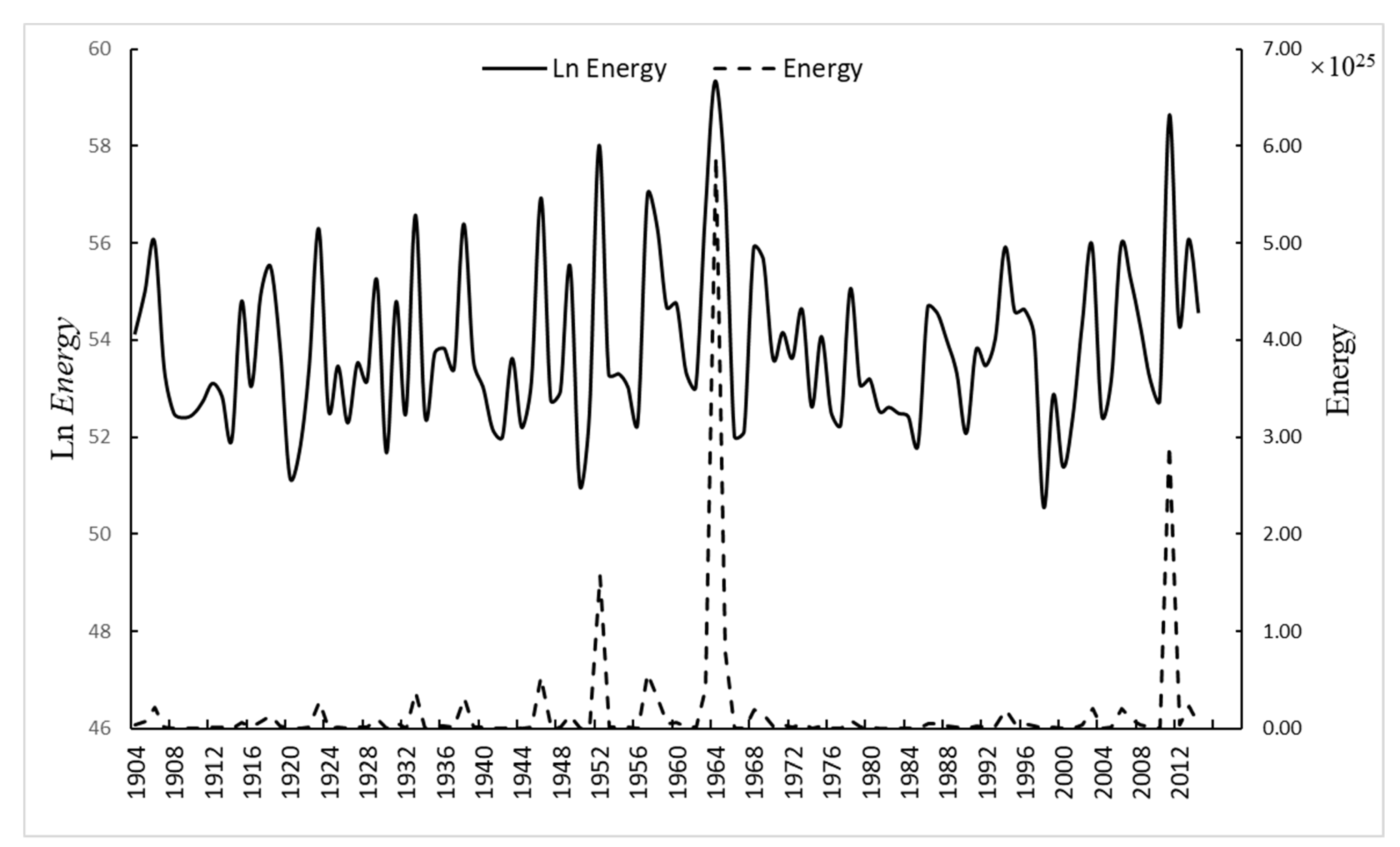
3.2. Stationarity Test of Energy Release
3.3. Results of the Causality Test between Plate Boundaries
4. Discussion
5. Conclusions
Author Contributions
Funding
Institutional Review Board Statement
Informed Consent Statement
Data Availability Statement
Conflicts of Interest
References
- Maruyama, S.; Santosh, M.; Zhao, D. Superplume, supercontinent, and post-perovskite: Mantle dynamics and anti-plate tectonics on the core-mantle boundary. Gondwana Res. 2007, 11, 7–37. [Google Scholar] [CrossRef]
- Le Pichon, X. Sea-floor spreading and continental drift. J. Geophys. Res. 1968, 73, 3661–3697. [Google Scholar] [CrossRef]
- Chase, C. The N plate problem of plate tectonics. Geophys. J. Int. 1972, 29, 117–122. [Google Scholar] [CrossRef]
- Minster, J.; Jordan, T.; Molnar, P.; Haines, E. Numerical modelling of instantaneous plate tectonics. Geophys. J. R. Astron. Soc. 1974, 36, 541–576. [Google Scholar] [CrossRef] [Green Version]
- Chase, C.G. Plate kinematics: The Americas, East Africa, and the rest of the world. Earth Planet. Sci. Lett. 1978, 37, 355–368. [Google Scholar] [CrossRef]
- DeMets, C.; Gordon, R.G.; Argus, D.F.; Stein, S. Effect of recent revisions to the geomagnetic reversal time scale on estimates of current plate motions. Geophys. Res. Lett. 1994, 21, 2191–2194. [Google Scholar] [CrossRef]
- Ren, Q.; Zhang, S.; Wu, H.; Liang, Z.; Miao, X.; Zhao, H.; Li, H.; Yang, T.; Pei, J.; Davis, G.A. Further paleomagnetic results from the ~155 Ma Tiaojishan formation, Yanshan Belt, North China, and their implications for the tectonic evolution of the Mongol-Okhotsk suture. Gondwana Res. 2016, 35, 180–191. [Google Scholar] [CrossRef]
- Metelkin, D.V.; Vernikovsky, V.A.; Kazansky, A.Y.; Wingate, M.T. Late Mesozoic tectonics of Central Asia based on paleomagnetic evidence. Gondwana Res. 2010, 18, 400–419. [Google Scholar] [CrossRef]
- Zhang, S.; Li, Z.-X.; Evans, D.A.; Wu, H.; Li, H.; Dong, J. Pre-Rodinia supercontinent Nuna shaping up: A global synthesis with new paleomagnetic results from North China. Earth Planet. Sci. Lett. 2012, 353, 145–155. [Google Scholar] [CrossRef]
- Yang, T.; Ma, Y.; Zhang, S.; Bian, W.; Yang, Z.; Wu, H.; Li, H.; Chen, W.; Ding, J. New insights into the India-Asia collision process from Cretaceous paleomagnetic and geochronologic results in the Lhasa terrane. Gondwana Res. 2015, 28, 625–641. [Google Scholar] [CrossRef]
- Kreemer, C.; Holt, W.E.; Haines, A.J. An integrated global model of present-day plate motions and plate boundary deformation. Geophys. J. Int. 2003, 154, 8–34. [Google Scholar] [CrossRef] [Green Version]
- Collilieux, X.; Altamimi, Z.; Coulot, D.; Ray, J.; Sillard, P. Comparison of very long baseline interferometry, GPS, and satellite laser ranging height residuals from ITRF2005 using spectral and correlation methods. J. Geophys. Res. Solid Earth 2007, 112. [Google Scholar] [CrossRef] [Green Version]
- Boehm, J.; Werl, B.; Schuh, H. Troposphere mapping functions for GPS and very long baseline interferometry from European Centre for Medium-Range Weather Forecasts operational analysis data. J. Geophys. Res. Solid Earth 2006, 111. [Google Scholar] [CrossRef]
- Condie, K.C. Archean geotherms and supracrustal assemblages. Tectonophysics 1984, 105, 29–41. [Google Scholar] [CrossRef]
- Condie, K.C. Plate Tectonics & Crustal Evolution; Elsevier: Amsterdam, The Netherlands, 2013. [Google Scholar]
- Milanovsky, E. Aulacogens of ancient platforms: Problems of their origin and tectonic development. In Developments in Geotectonics; Elsevier: Amsterdam, The Netherlands, 1981; Volume 17, pp. 213–248. [Google Scholar]
- Glikson, A. Precambrian sial-sima relations: Evidence for Earth expansion. Tectonophysics 1980, 63, 193–234. [Google Scholar] [CrossRef]
- Blackett, P.M.S. A negative experiment relating to magnetism and the earth’s rotation. Phil. Trans. R. Soc. Lond. A 1952, 245, 309–370. [Google Scholar]
- Bullard, E.; Everett, J.E.; Smith, A.G. The fit of the continents around the Atlantic. Phil. Trans. R. Soc. Lond. A 1965, 258, 41–51. [Google Scholar] [CrossRef]
- Dietz, R.S. Continent and ocean basin evolution by spreading of the sea floor. Nature 1961, 190, 854–857. [Google Scholar] [CrossRef]
- Wilson, J.T. A new class of faults and their bearing on continental drift. Nature 1965, 207, 343. [Google Scholar] [CrossRef]
- Marvin, U.B. Continents adrift: Readings from Scientific American. J. Geol. 1973, 81, 520–521. [Google Scholar] [CrossRef]
- Morgan, W.J. Convection plumes in the lower mantle. Nature 1971, 230, 42. [Google Scholar] [CrossRef]
- Sleep, N.H. Hotspots and mantle plumes: Some phenomenology. J. Geophys. Res. Solid Earth 1990, 95, 6715–6736. [Google Scholar] [CrossRef]
- Larson, R. Latest pulse of Earth: Evidence for a mid-Cretaceous superplume. Geology 1991, 19, 547–550. [Google Scholar] [CrossRef]
- Stein, M.; Hofmann, A. Mantle plumes and episodic crustal growth. Nature 1994, 372, 63. [Google Scholar] [CrossRef]
- Meyerhoff, A.A.; Taner, I.; Morris, A.; Agocs, W.; Kamen-Kaye, M.; Bhat, M.I.; Smoot, N.C.; Choi, D.R. Surge Tectonics: A New Hypothesis of Global Geodynamics; Springer Science & Business Media: Berlin/Heidelberg, Germany, 1996; Volume 9. [Google Scholar]
- Backus, G.; Park, J.; Garbasz, D. On the relative importance of the driving forces of plate motion. Geophys. J. R. Astron. Soc. 1981, 67, 415–435. [Google Scholar] [CrossRef] [Green Version]
- Conrad, C.P.; Lithgow-Bertelloni, C. How mantle slabs drive plate tectonics. Science 2002, 298, 207–209. [Google Scholar] [CrossRef]
- McKenzie, D.P. Speculations on the consequences and causes of plate motions. Geophys. J. R. Astron. Soc. 1969, 18, 1–32. [Google Scholar] [CrossRef] [Green Version]
- Schellart, W. Quantifying the net slab pull force as a driving mechanism for plate tectonics. Geophys. Res. Lett. 2004, 31. [Google Scholar] [CrossRef] [Green Version]
- Forsyth, D.; Uyedaf, S. On the relative importance of the driving forces of plate motion. Geophys. J. R. Astron. Soc. 1975, 43, 163–200. [Google Scholar] [CrossRef] [Green Version]
- Parmentier, E.; Turcotte, D.; Torrance, K. Studies of finite amplitude non-Newtonian thermal convection with application to convection in the Earth’s mantle. J. Geophys. Res. 1976, 81, 1839–1846. [Google Scholar] [CrossRef]
- Stadler, G.; Gurnis, M.; Burstedde, C.; Wilcox, L.C.; Alisic, L.; Ghattas, O. The dynamics of plate tectonics and mantle flow: From local to global scales. Science 2010, 329, 1033–1038. [Google Scholar] [CrossRef]
- Larter, R.D.; Barker, P.F. Effects of ridge crest-trench interaction on Antarctic-Phoenix spreading: Forces on a young subducting plate. J. Geophys. Res. Solid Earth 1991, 96, 19583–19607. [Google Scholar] [CrossRef]
- Wiener, N. The theory of prediction. Mod. Math. Eng. 1956. [Google Scholar]
- Granger, C.W. Investigating causal relations by econometric models and cross-spectral methods. Econom. J. Econom. Soc. 1969, 424–438. [Google Scholar] [CrossRef]
- Granger, C.W. Testing for causality: A personal viewpoint. J. Econ. Dyn. Control 1980, 2, 329–352. [Google Scholar] [CrossRef]
- Bozoklu, S.; Yilanci, V. Energy consumption and economic growth for selected OECD countries: Further evidence from the Granger causality test in the frequency domain. Energy Policy 2013, 63, 877–881. [Google Scholar] [CrossRef]
- Akinboade, O.A.; Braimoh, L.A. International tourism and economic development in South Africa: A Granger causality test. Int. J. Tour. Res. 2010, 12, 149–163. [Google Scholar] [CrossRef]
- Kónya, L. Exports and growth: Granger causality analysis on OECD countries with a panel data approach. Econ. Model. 2006, 23, 978–992. [Google Scholar] [CrossRef]
- Ghosh, S. Electricity consumption and economic growth in India. Energy Policy 2002, 30, 125–129. [Google Scholar] [CrossRef]
- Dufour, J.-M.; Renault, E. Short run and long run causality in time series: Theory. Econometrica 1998, 1099–1125. [Google Scholar] [CrossRef]
- Engle, R.F.; Granger, C.W. Co-integration and error correction: Representation, estimation, and testing. Econom. J. Econom. Soc. 1987, 251–276. [Google Scholar] [CrossRef]
- Granger, C.W. Causality, cointegration, and control. J. Econ. Dyn. Control 1988, 12, 551–559. [Google Scholar] [CrossRef]
- Phillips, P.C.; Perron, P. Testing for a unit root in time series regression. Biometrika 1988, 75, 335–346. [Google Scholar] [CrossRef]
- Storchak, D.A.; Di Giacomo, D.; Bondár, I.; Engdahl, E.R.; Harris, J.; Lee, W.H.; Villaseñor, A.; Bormann, P. Public release of the ISC–GEM global instrumental earthquake catalogue (1900–2009). Seismol. Res. Lett. 2013, 84, 810–815. [Google Scholar] [CrossRef] [Green Version]
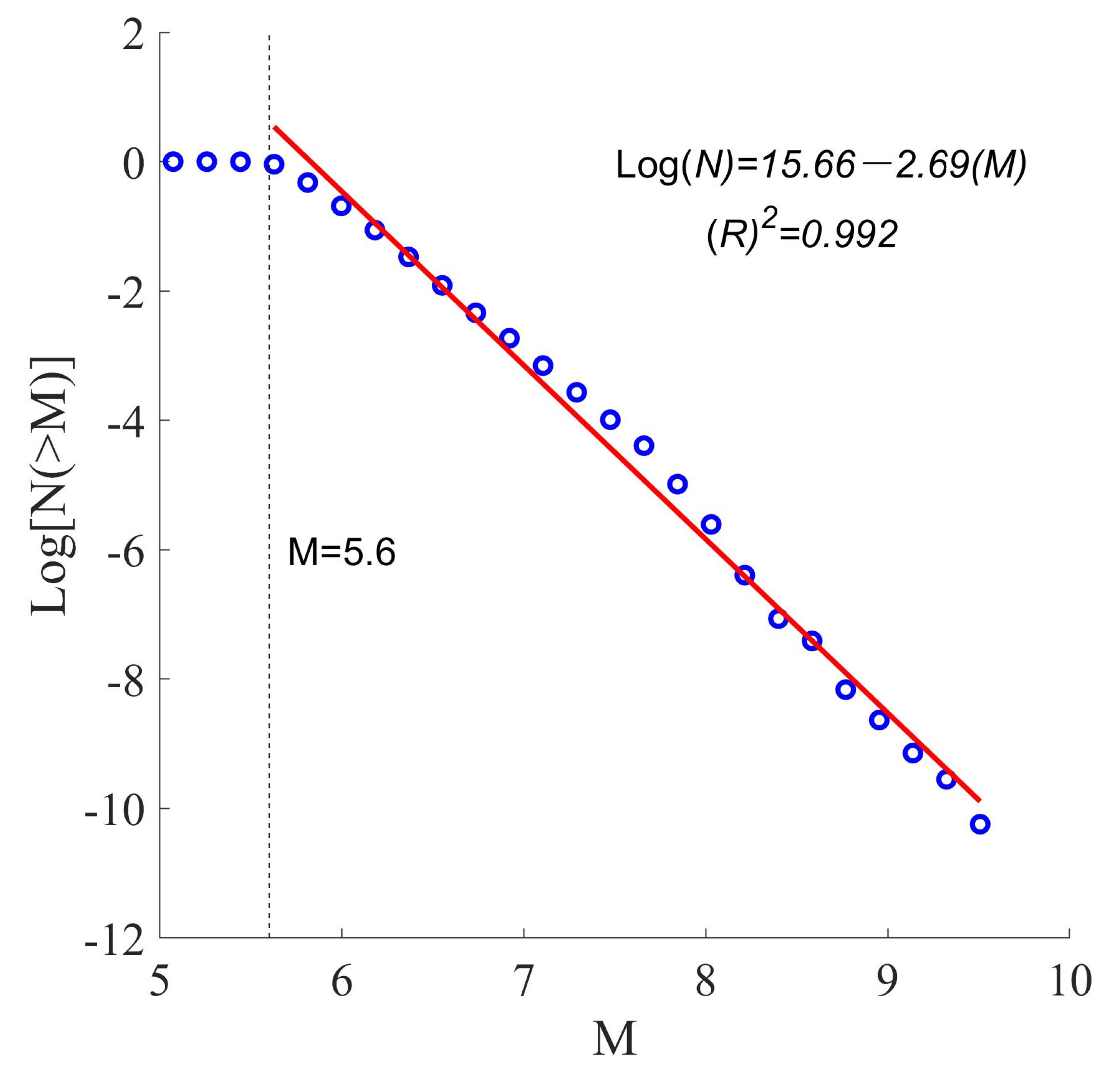
- Cheng, Q.-M.; Sun, H.-Y. Variation of singularity of earthquake-size distribution with respect to tectonic regime. Geosci. Front. 2018, 9, 453–458. [Google Scholar] [CrossRef]
- Wiemer, S.; Wyss, M. Minimum magnitude of completeness in earthquake catalogs: Examples from Alaska, the western United States, and Japan. Bull. Seismol. Soc. Am. 2000, 90, 859–869. [Google Scholar] [CrossRef]
- Woessner, J.; Wiemer, S. Assessing the quality of earthquake catalogues: Estimating the magnitude of completeness and its uncertainty. Bull. Seismol. Soc. Am. 2005, 95, 684–698. [Google Scholar] [CrossRef]
- Gutenberg, B.; Richter, C.F. Frequency of earthquakes in California. Bull. Seismol. Soc. Am. 1944, 34, 185–188. [Google Scholar] [CrossRef]
- Bird, P. An updated digital model of plate boundaries. Geochem. Geophys. Geosyst. 2003, 4. [Google Scholar] [CrossRef]
- Hall, T.R.; Nixon, C.W.; Keir, D.; Burton, P.W.; Ayele, A. Earthquake clustering and energy release of the African-Arabian rift system. Bull. Seismol. Soc. Am. 2018, 108, 155–162. [Google Scholar] [CrossRef] [Green Version]
- Hanks, T.C.; Kanamori, H. A moment magnitude scale. J. Geophys. Res. Solid Earth 1979, 84, 2348–2350. [Google Scholar] [CrossRef]
- Dickey, D.A.; Fuller, W.A. Distribution of the estimators for autoregressive time series with a unit root. J. Am. Stat. Assoc. 1979, 74, 427–431. [Google Scholar]
- Dickey, D.A.; Fuller, W.A. Likelihood ratio statistics for autoregressive time series with a unit root. Econom. J. Econom. Soc. 1981, 1057–1072. [Google Scholar] [CrossRef]
- Balcilar, M.; Ozdemir, Z.A. The export-output growth nexus in Japan: A bootstrap rolling window approach. Empir. Econ. 2013, 44, 639–660. [Google Scholar] [CrossRef]
- Altamimi, Z.; Métivier, L.; Collilieux, X. ITRF2008 plate motion model. J. Geophys. Res. Solid Earth 2012, 117. [Google Scholar] [CrossRef]
- Prawirodirdjo, L.; Bock, Y. Instantaneous global plate motion model from 12 years of continuous GPS observations. J. Geophys. Res. Solid Earth 2004, 109. [Google Scholar] [CrossRef]
- Iaffaldano, G.; Bunge, H.-P. Relating rapid plate-motion variations to plate-boundary forces in global coupled models of the mantle/lithosphere system: Effects of topography and friction. Tectonophysics 2009, 474, 393–404. [Google Scholar] [CrossRef]
- Zhong, S.; Gurnis, M. Mantle convection with plates and mobile, faulted plate margins. Science 1995, 267, 838–843. [Google Scholar] [CrossRef]
- Copley, A.; Avouac, J.P.; Royer, J.Y. India-Asia collision and the Cenozoic slowdown of the Indian plate: Implications for the forces driving plate motions. J. Geophys. Res. Solid Earth 2010, 115. [Google Scholar] [CrossRef] [Green Version]
- Cande, S.C.; Stegman, D.R. Indian and African plate motions driven by the push force of the Reunion plume head. Nature 2011, 475, 47. [Google Scholar] [CrossRef]

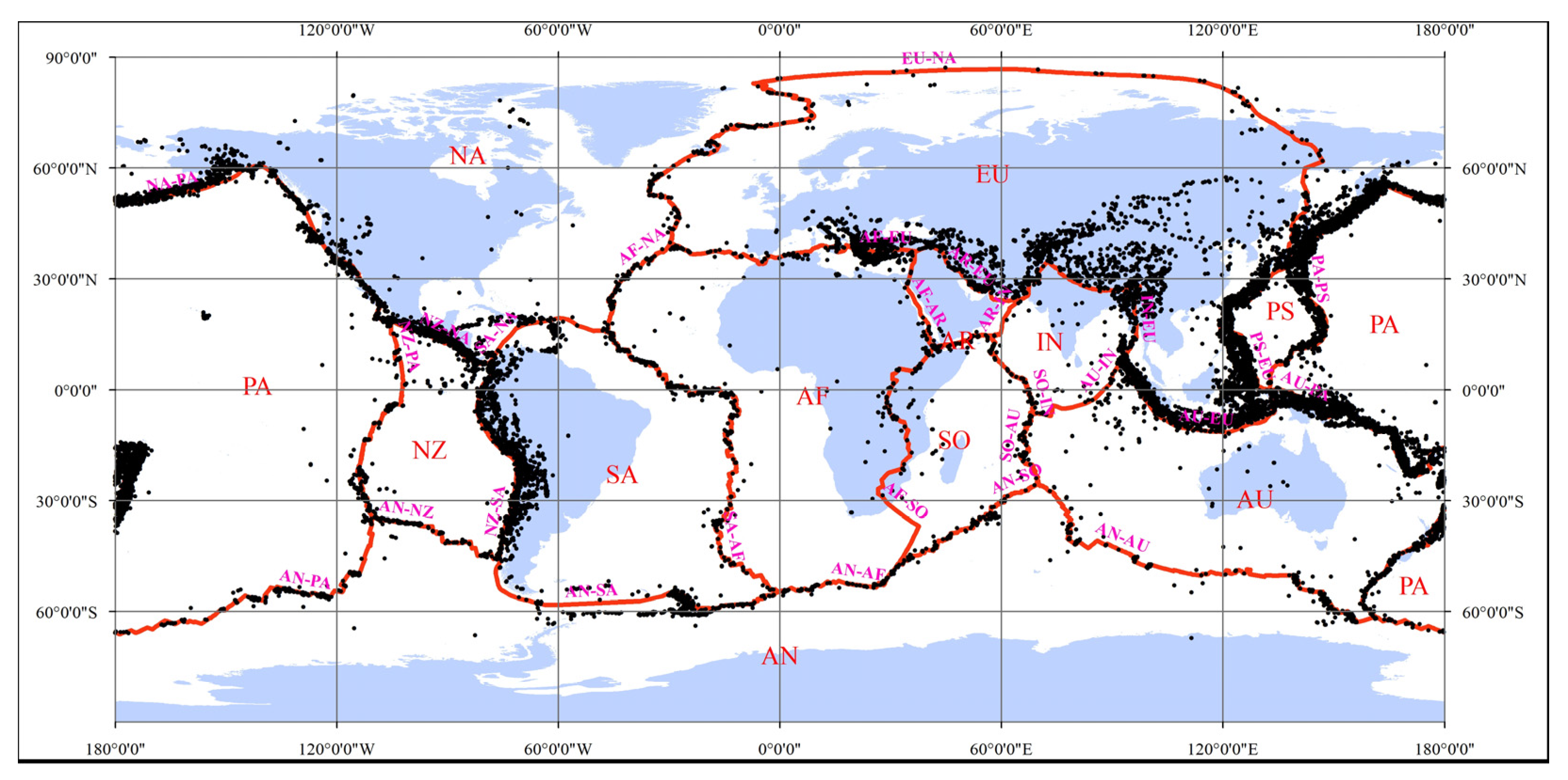
| Boundary name | NA-PA | NZ-PA | AN-PA | AU-PA | NZ-NA | NZ-SA | AN-NZ | SA-NA | SA-AF | AN-SA | AF-NA | AF-EU | AF-AR | AF-SO |
| Earthquake Number | 4479 | 283 | 275 | 6305 | 1017 | 1569 | 169 | 296 | 455 | 469 | 106 | 458 | 56 | 107 |
| Energy release | 1.75 × 1026 | 2.2 × 10²³ | 1.71 × 10²³ | 5.16 × 1025 | 1.07 × 1025 | 2.21 × 1026 | 1.51 × 10²³ | 1.49 × 1024 | 8.18 × 10²³ | 3.28 × 1024 | 5.79 × 10²² | 3.81 × 1024 | 8.32 × 10²² | 2.56 × 10²³ |
| Boundary name | AN-AF | AR-EU | AR-IN | SO-AR | SO-IN | SO-AU | AN-SO | IN-EU | AU-IN | AU-EU | AN-AU | PA-PS | PS-EU | EU-NA |
| Earthquake Number | 84 | 387 | 7 | 57 | 65 | 84 | 121 | 1346 | 91 | 1507 | 355 | 681 | 2871 | 422 |
| Energy release | 7.24 × 10²³ | 2.4 × 1024 | 9.09 × 10²⁰ | 2.95 × 10²² | 1.82 × 10²³ | 5.42 × 10²² | 3.89 × 10²³ | 1.78 × 1025 | 2.39 × 1024 | 5.12 × 1025 | 1.23 × 1024 | 3.39 × 1024 | 2.87 × 1025 | 2.52 × 1024 |
| Boundary name | AF-AR | AF-EU | AF-NA | AF-SO | AN-AF | AN-AU | AN-NZ | AN-PA | AN-SA | AN-SO | AR-EU | AR-IN | AU-EU | AU-IN |
| ADF statistic | −10.52 *** | −12.393 *** | −8.244 *** | −10.45 *** | −11.275 *** | −7.871 *** | −11.24067 *** | −10.595 *** | −8.655 *** | −8.908 *** | −11.9 *** | −11.079 *** | −14.159 *** | −10.898 *** |
| Order of integration | 0 | 0 | 0 | 0 | 0 | 0 | 0 | 0 | 0 | 0 | 0 | 0 | 0 | 0 |
| Boundary name | AU-PA | EU-NA | IN-EU | NA-PA | NZ-NA | NZ-PA | NZ-SA | PA-PS | PS-EU | SA-AF | SA-NA | SO-AR | SO-AU | SO-IN |
| ADF statistic | −13.002 *** | −10.892 *** | −32.275 *** | −9.021 *** | −10.406 *** | −5.686 *** | −10.255 *** | −4.916 *** | −42.734 *** | −6.758 *** | −10.183 *** | −8.643 *** | −11.015 *** | −10.683 *** |
| Order of integration | 0 | 0 | 0 | 0 | 0 | 0 | 0 | 0 | 0 | 0 | 0 | 0 | 0 | 0 |
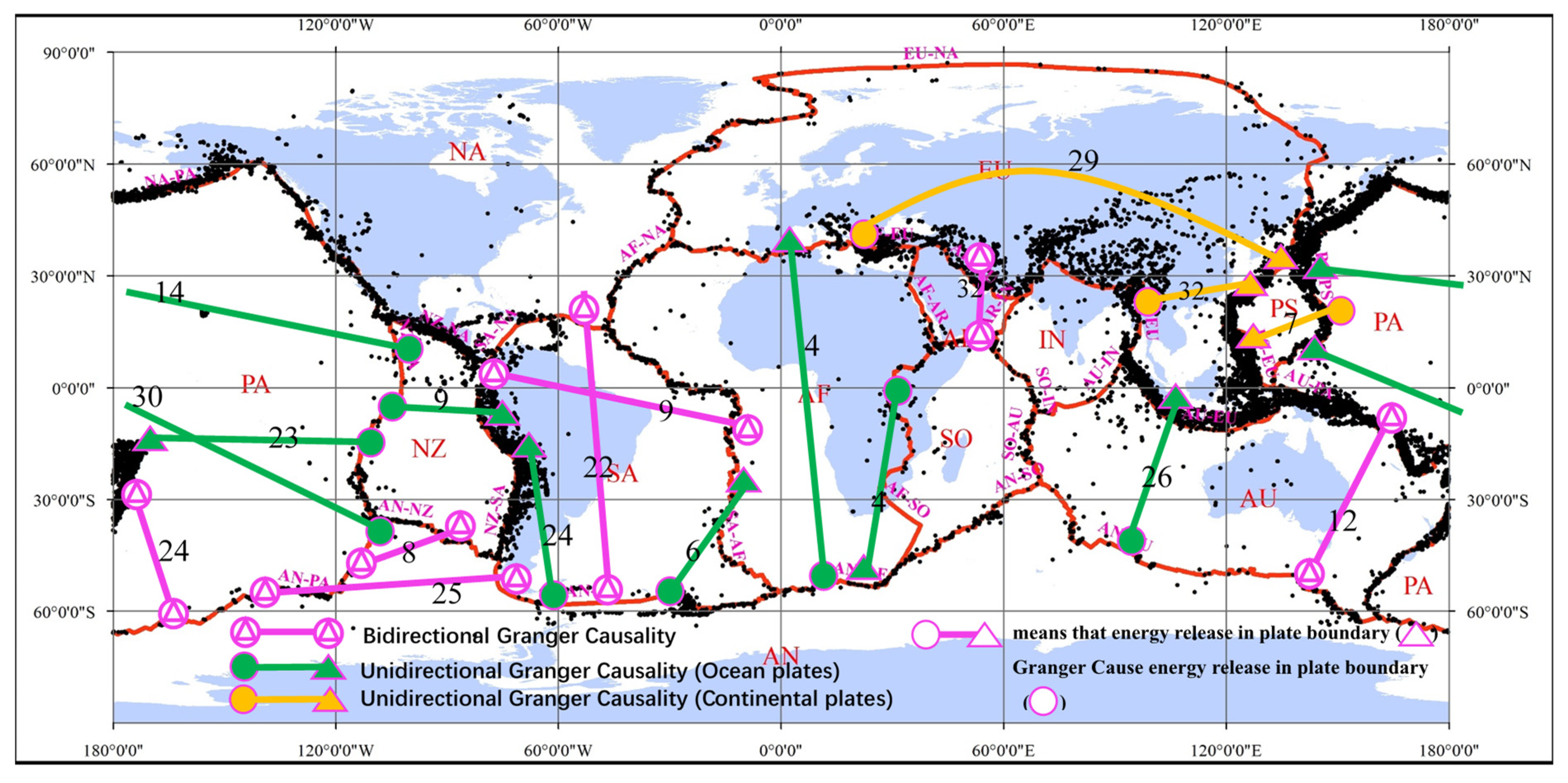
| Direction of Causality | Granger Test | Cointegration Test | ||||
|---|---|---|---|---|---|---|
| From | To | F-Statistics | P | Lag Length | Statistics | P |
| NZ-PA | PA-PS | 11.68343 | 0.6317 | 14 | −6.609 | 0 |
| PA-PS | NZ-PA | 24.52843 | 0.0395 | 14 | ||
| AN-PA | PA-PS | 21.36072 | 0.8763 | 30 | −4.647 | 0.001 |
| PA-PS | AN-PA | 69.31429 | 0.0001 | 30 | ||
| NZ-PA | AU-PA | 19.72928 | 0.6582 | 23 | −4.96 | 0.001 |
| AU-PA | NZ-PA | 38.60992 | 0.0219 | 23 | ||
| AN-PA | AU-PA | 60.61951 | 0.0001 | 24 | −7.365 | 0 |
| AU-PA | AN-PA | 46.5939 | 0.0038 | 24 | ||
| NZ-PA | NZ-SA | 8.091878 | 0.5249 | 9 | −5.243 | 0 |
| NZ-SA | NZ-PA | 23.13383 | 0.0059 | 9 | ||
| AN-SA | SA-NA | 43.688 | 0.0039 | 22 | −3.932 | −0.012 |
| SA-NA | AN-SA | 49.71639 | 0.0006 | 22 | ||
| AN-SA | NZ-SA | 31.60144 | 0.1372 | 24 | −4.044 | 0.009 |
| NZ-SA | AN-SA | 67.6177 | 0 | 24 | ||
| NZ-SA | SA-AF | 66.31497 | 0 | 9 | −11.09 | 0 |
| SA-AF | NZ-SA | 125.734 | 0 | 9 | ||
| AN-SA | SA-AF | 3.560421 | 0.7359 | 6 | −5.298 | 0 |
| SA-AF | AN-SA | 16.40422 | 0.0117 | 6 | ||
| AN-AF | AF-SO | 12.18294 | 0.0166 | 4 | −8.485 | 0 |
| AF-SO | AN-AF | 2.911122 | 0.5728 | 4 | ||
| AN-AF | AF-EU | 6.970334 | 0.1375 | 4 | −8.45 | 0 |
| AF-EU | AN-AF | 8.452415 | 0.0763 | 4 | ||
| SO-AR | AR-EU | 43.16792 | 0.0899 | 32 | −8.652 | 0 |
| AR-EU | SO-AR | 45.15261 | 0.0615 | 32 | ||
| PA-PS | PS-EU | 8.290653 | 0.3077 | 7 | −5.19 | 0 |
| PS-EU | PA-PS | 20.3014 | 0.005 | 7 | ||
| AF-EU | PS-EU | 29.18502 | 0.4555 | 29 | −10.875 | 0 |
| PS-EU | AF-EU | 58.76574 | 0.0009 | 29 | ||
| IN-EU | PS-EU | 14.77975 | 0.996 | 32 | −10.156 | 0 |
| PS-EU | IN-EU | 54.48406 | 0.0079 | 32 | ||
| AN-PA | AN-NZ | 15.00008 | 0.0591 | 8 | −10.671 | 0 |
| AN-NZ | AN-PA | 19.33468 | 0.0132 | 8 | ||
| AN-PA | AN-SA | 112.5939 | 0 | 25 | −5.414 | 0 |
| AN-SA | AN-PA | 109.1282 | 0 | 25 | ||
| AN-AU | AU-EU | 21.11864 | 0.7358 | 26 | −2.564 | 0.26 |
| AU-EU | AN-AU | 97.2081 | 0 | 26 | ||
| AN-AU | AU-PA | 28.10634 | 0.0053 | 12 | −2.492 | 0.29 |
| AU-PA | AN-AU | 45.1501 | 0 | 12 | ||
Publisher’s Note: MDPI stays neutral with regard to jurisdictional claims in published maps and institutional affiliations. |
© 2021 by the authors. Licensee MDPI, Basel, Switzerland. This article is an open access article distributed under the terms and conditions of the Creative Commons Attribution (CC BY) license (https://creativecommons.org/licenses/by/4.0/).
Share and Cite
Ning, L.; Hui, C.; Cheng, C. Exploring the Dynamics of Global Plate Motion Based on the Granger Causality Test. Appl. Sci. 2021, 11, 7853. https://doi.org/10.3390/app11177853
Ning L, Hui C, Cheng C. Exploring the Dynamics of Global Plate Motion Based on the Granger Causality Test. Applied Sciences. 2021; 11(17):7853. https://doi.org/10.3390/app11177853
Chicago/Turabian StyleNing, Lixin, Chun Hui, and Changxiu Cheng. 2021. "Exploring the Dynamics of Global Plate Motion Based on the Granger Causality Test" Applied Sciences 11, no. 17: 7853. https://doi.org/10.3390/app11177853
APA StyleNing, L., Hui, C., & Cheng, C. (2021). Exploring the Dynamics of Global Plate Motion Based on the Granger Causality Test. Applied Sciences, 11(17), 7853. https://doi.org/10.3390/app11177853