Article

Designing of the Tracks and Modeling of the Carrier Arrangement in Square Rotary Braiding Machine

1
College of Mechanical Engineering, Donghua University, Shanghai 201620, China
2
Engineering Research Center of Advanced Textile Machinery, Ministry of Education, Donghua University, Shanghai 201620, China
3
Hangchen Shijiazhuang New Material Technology Co., Ltd., Shijiazhuang 051430, China
*
Author to whom correspondence should be addressed.
Appl. Sci. 2021, 11(17), 7861; https://doi.org/10.3390/app11177861
Submission received: 8 July 2021 / Revised: 20 August 2021 / Accepted: 24 August 2021 / Published: 26 August 2021

Abstract

:
This paper describes the splicing of an 8 × 8 484 cross-break track, based on the carrier arrangement characteristics (CAC) method for track splicing technology. The arrangement period of the carrier (T) in the track is obtained in order to discern which slot has a carrier in a period and which one does not. Six basic types of track unit are deconstructed, and a mathematical model is established to determine the possible state of the carrier in each slot of the track unit. Finally, the specific pattern of the carrier arrangement in the 484 cross-break track unit is obtained and verified using a three-dimensional (3D) rotary braiding machine with a square track disc. This provides a reference for solving the carrier arrangement of a 3D square rotary braiding machine.

1. Introduction

Three-dimensional (3D) braiding technology was first developed in the 1970s, in the United States, through the successful application of 3D braiding a composite material to replace the alloy material of rocket engines [1]. The 3D fabric braided by this technology is lightweight, with high levels of strength and integrity [2]. This successful application demonstrated the development potential of 3D braiding materials. In the last 10 years, 3D braiding technology has gradually been adopted in various fields, such as aerospace [3], automobiles [4], and medical treatment [5,6,7], among others [8].
Three-dimensional braided fabric has the characteristics of multi-directional fiber orientation and an overall continuous distribution, which endows 3D braided composites with a series of excellent mechanical properties. Three-dimensional braiding technology has a strong ability to realize the complete braiding of complex structures. In the traditional 3D braiding process, variously shaped cross-sections of the preform can be flexibly braided by changing the arrangement shape of the carrier and increasing or decreasing the number of braided yarns [9]. Kostar et al. [10,11] analyzed two-step, four-step, and multi-step Cartesian track and column braids, and developed a computer algorithm to determine the corresponding process for braiding when given the desired cross-section shape. In addition, the algorithm can also calculate the steps needed to form the braided fabric with special cross-sectional shapes, such as fasteners, surrogate materials, and voids. The algorithm was combined with a multi-step braiding machine, and several different braided fabrics were produced with alternative materials. However, this method necessitates precise control of the external dimensions, which often requires the use of computer-based iterative arithmetic or trial-and-error based on experience. In recent years, research on 3D braided composite molding equipment in developed countries has made great progress. As the braiding procedure dictates the yarn structure in the preform, and the yarn structure dictates the properties of the composite, a preform can be designed. Three-dimensional braided fabrics are composed of yarns, interlaced in order spatially. The main structural parameters are the braiding angle, surface braiding angle, node height, and fiber volume fraction. The study of braiding structure is mainly used to establish its theoretical model, obtain its structural parameters, and analyze its mechanical properties, by analyzing the interlacing of internal yarns. Since 1985, 3D braiding technology has made great progress, and the four-step method has gradually formed the basis of the braiding process. However, fabric structures with differently-shaped cross-sections are mainly obtained by changing the arrangement of the carriers and the number of cyclic steps. Based on the four-step 3D braiding process with a rectangular cross-section, Yuling et al. [12,13] summarized the principles of the arrangement of yarn carriers in the braiding process of fabric with an irregular cross-section. During in the 21st century, the rotary 3D braiding machine was developed and quickly became a mainstream braiding technology tool, represented by two core braiding technologies [14]. Mungalov et al. [15] described the relationship between the cross-sectional shape of a 3D-braided preform and the gripping fork actuation. Tolosana et al. [16] developed a new software to emulate the operation of the rotary braiding machine. Tada et al. [17] derived a formula to determine the optimal number of bundles for flat and hollow square braids.
In their research into the track splicing of rotary braiding, Akiyama et al. [18] applied the track-splicing mechanism to the field of braiding. They described the production of an H-beam form by adding forks and transfer tracks among three different linear sections. However, the added transfer tracks limited the cross-sectional shape of the fabric; that is, a machine could produce only one cross-section fabric shape. Kyosev presented the production of braids with square cross-sectional forms using a rotary braiding technique in [19]. For the four-slot horn gears, with the increase in the fabric size, especially when three or more tracks were used (Tracks 1, 2, and 3 in Figure 1) for braiding, the one full (“1”) one empty (“0”) arrangement (“10”) of the carriers is impossible; that is, it is impossible to place half the slots of all horn gears (called the full carrier arrangement of carriers, in this paper) with carriers at the same time. The collision problem between the carriers can only be solved by reducing the number of carriers, such as in the one full (“1”) arrangement (T − 1) empty (“ 0 0 T 1 ”) (“ 1   0 0 T 1 ”) arrangement results in a lower utilization rate for the slot. The latest book by Kyosev [20] provides a carrier motion that is emulated by combining track- and horn gear-based modeling methods, and the application of this method has been detailed in [21,22,23]. The commercial software TexMind can check the braiding carrier configurations; however, this approach is carried out under the assumption that the carrier configuration is working, and the aim of this paper is to obtain the configuration (arrangement) of the carrier in the tracks using a mathematical model, in order to avoid the collision problem.
This paper describes the splicing of an 8 × 8 484 cross-break track (explained in detail in Section 2.2), based on the method stated in [24], which was proposed by the authors. A mathematical model of the carrier arrangement is established in order to obtain the specific pattern of the carrier arrangement in a period, which can help engineers to design larger 3D rotary braiding machines with square-shaped configuration track discs.

2. Track-Splicing Process

2.1. General Steps of Track Splicing

In order to save space, the main steps of the track-splicing method using the CAC method are as follows:
The carrier arrangement characteristics (CAC) method has been presented in [24]. It comprises the existence and arrangement characteristics of carriers in the horn gear slot in the tracks. It is a mathematical description of the carrier state in the slot of the track. The CAC is different from the “number of carrier arrangement characteristics”, and the CAC needs to be calculated first. Then, the “number for the carrier arrangement characteristics” is calculated second. Figure 2 shows the splicing mechanism from the first track unit (1) to the final one (j + 1).
(1)
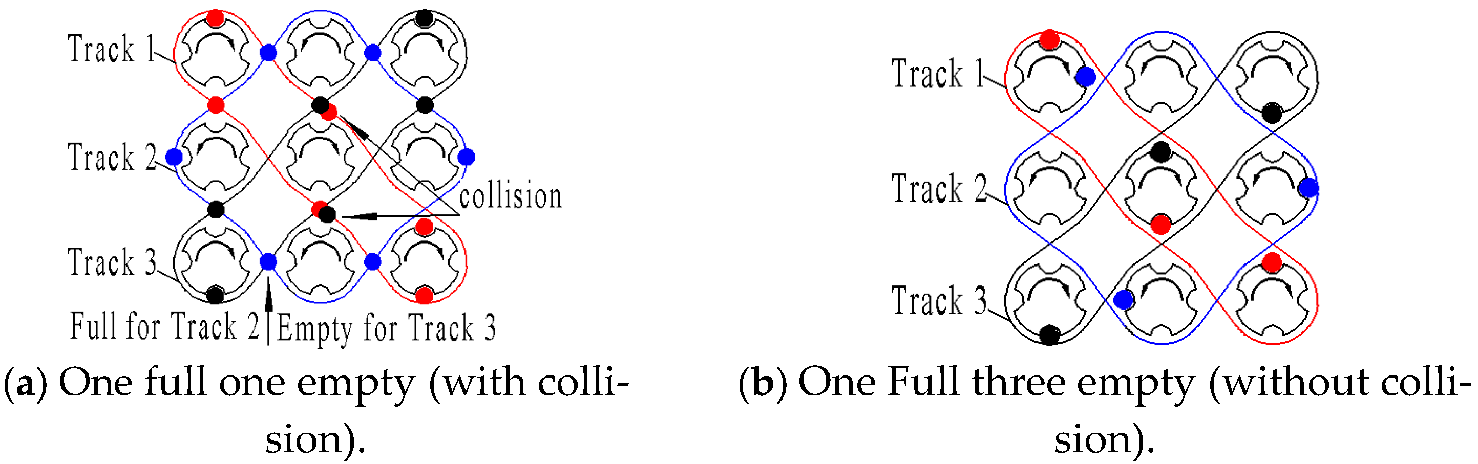
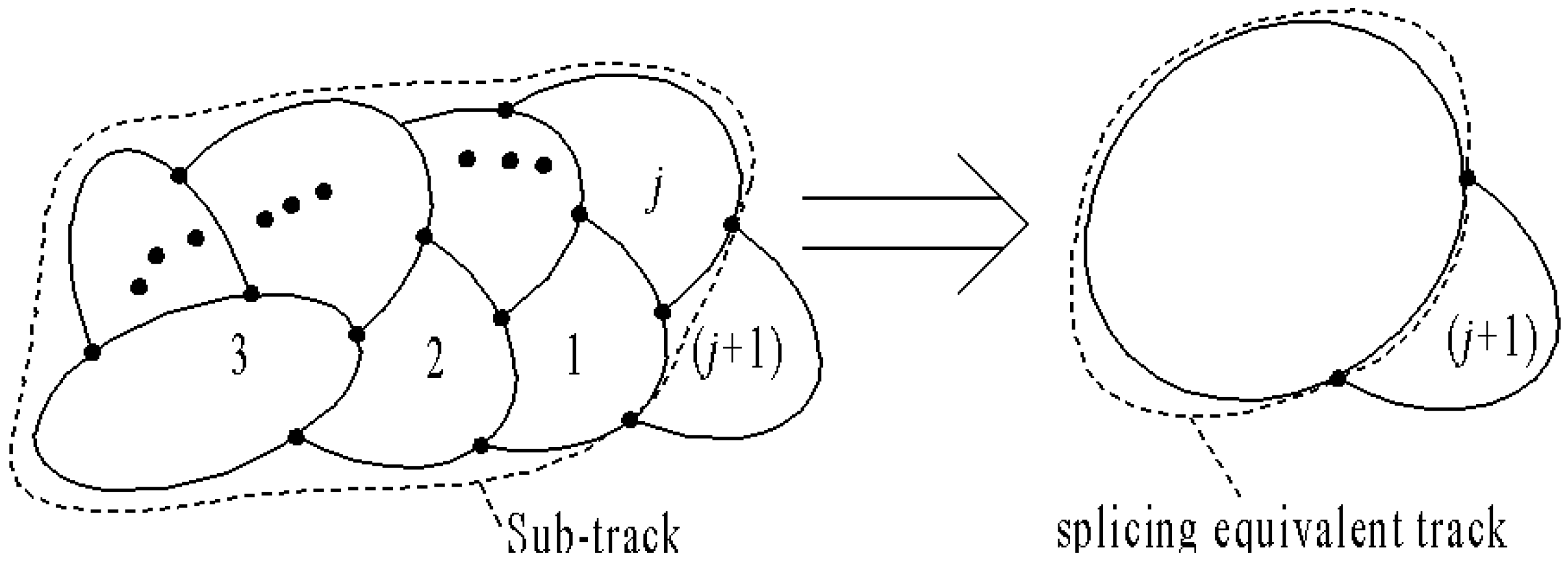
Determine the characteristics of the carrier arrangement in the 4 × 4 track ( M b i ). This step can determine the existence of the carriers in the 4 × 4 track units, indicated by 1, 2, 3, ..., (j + 1) in Figure 2, in the arrangement period. The characteristics of the carrier arrangement M b i represent the CAC set of carriers that do not collide with each other in the tracks, while the elements in M b i only represent the existence of the carriers in the slots in an arrangement period of the carrier.
(2)
Determine the characteristic number of carrier arrangement for track units 1, 2. This step can determine the number of carriers at the slots in the track composed of the first two track units (1 and 2 in Figure 2), called dim. {M} and the dim. {M} is the number of elements in the CAC, that is, the dimension of the CAC. There is no collision constraint between the carriers, and it is independent of the track unit number.
ξ L 1 = dim . { M b 1 M b 2 }
(3)
Determine the carrier arrangement characteristics of the first sub-track, composed of the first and second track units.
This step can determine the existence of the carriers in the first sub-track composed of the first track unit “1” and the second track unit “2”, as shown in Figure 2.
M pa ( 1 2 ) = M b 1 M b 2
(4)
Determine the characteristic carrier arrangement number of the first jth sub-track, composed of j track units ranging from the first track unit “1” to the jth track unit (j):
ξ L j = dim . { M P a ( 1 j ) M b ( j + 1 ) }
(5)
Determine the carrier arrangement characteristics of the track spliced by the first (j + 1) track units, where the existence of the carriers in the track units—from the first unit “1” to the final one (j + 1) in Figure 2—in the arrangement period is obtained:
M pa ( 1 ( j + 1 ) ) = M P a ( 1 j ) M b ( j + 1 )
(6)
Determine the arrangement period (T) of the carriers in the spliced track unit. f i is the summation of the ith track unit, m is the number of track units, and υ is the number of track loops. ξ L j indicates the number of carriers and the arrangement characteristics of the jth track unit (formed by the equivalent track units that are formed by the first j track units and the (j + 1)th track unit shown in Figure 2).
T = i = 1 m f i j υ ξ L j

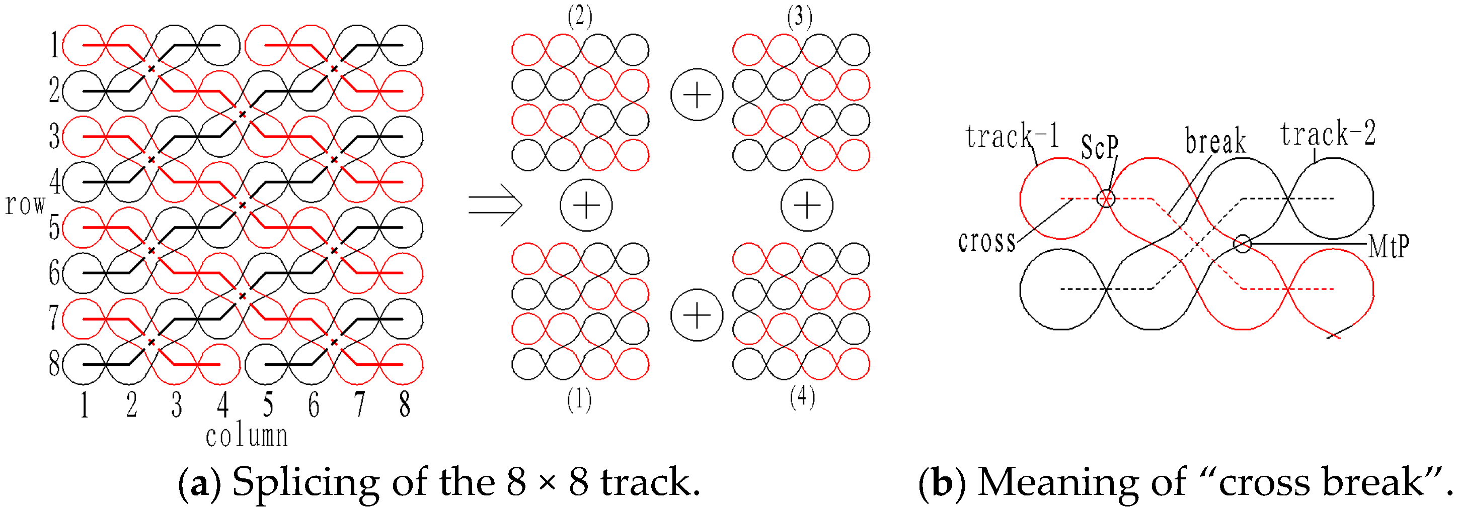
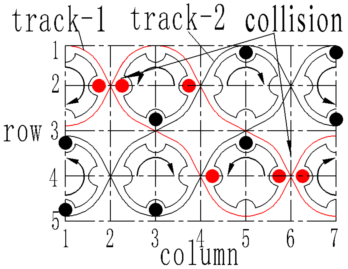
2.2. The Splicing Process of 8 × 8 484 Cross-Break Track

The splicing schematic of the 8 × 8 484 cross-break track is shown in Figure 3. It can be seen that the 8 × 8 484 cross-break track is composed of four 4 × 4484 cross-break track units: 4 × 4484 cross-break (1), 4 × 4484 cross-break (2), 4 × 4484 cross-break (3), and 4 × 4484 cross-break (4). As shown in Figure 3a, the numbers in brackets represent the order of track unit splicing, and 4 × 4 indicates that the track consists of four rows and four columns, with the horn gear configuration, for a total of 16 (16 = 4 × 4) horn gears. The number 484 represents that each track first includes a 4-slot horn gear, then connects a total of 8n-slots (8n = 4 × 2n, where n is a positive integer) horn gear system composed of a 2n 4-slot horn gears and, finally, connects a 4-slot horn gear. “Cross-break” means that the trajectory of the track first follows the horizontal direction (cross), then the +45° or −45° direction (break), as shown in Figure 3b. The meanings of ScP and MtP in Figure 3b are explained in Section 3.1.
(1)
Determine the CAC of the first to fourth 4 × 4 track units:
M b i = [ f 4 e 4 ] [ f 4 e 4 ] [ f 4 e 4 ] [ f 4 e 4 ] = [ f 4 e 4 ] ,   i = 1 , 2 , 3 , 4
(2)
Determine the CAC carrier arrangement number in the first sub-track, composed of track unit (1) and track unit (2):
ξ L 1 = dim . { [ f 4 e 4 ] [ f 1 e 1 ] [ f 4 e 4 ] } = 3
(3)
Determine the CAC of track unit (1) and track unit (2):
M T R 1 2 = M b 1 M b 2 = [ f 4 e 4 ] [ f 4 e 4 ] = [ f 4 e 4 ]
(4)
Determine the CAC carrier arrangement number in the second sub-track, consisting of track units (1), (2), and (3):
ξ L 2 = dim . { [ f 4 e 4 ] [ f 1 e 1 ] [ f 4 e 4 ] [ f 4 e 4 ] } = 4
(5)
Determine the CAC of track unit (1), track unit (2), and track unit (3):
M T R 1 3 = M T R 1 2 M b 3 = [ f 4 e 4 ] [ f 4 e 4 ] = [ f 4 e 4 ]
(6)
Determine the CAC number in the third sub-track, which consists of track units (1), (2), (3), and (4):
ξ L 3 = dim . { [ f 4 e 4 ] [ f 1 e 1 ] [ f 4 e 4 ] [ f 4 e 4 ] [ f 1 e 1 ] [ f 4 e 4 ] } = 6
(7)
Determine the arrangement period of the carrier in the 8 × 8 484 cross-break track:
T T R * = i = 1 4 f i j = 1 3 ξ L j = 21 ( 3 + 4 + 6 ) = 8
Therefore, the arrangement period of the carrier in the 8 × 8 484 cross-break track is 8, and its CAC set is [ f 4 e 4 ] T . However, in each 484 cross-break track units obtained by applying the method in [24], it is not possible to determine which of the eight adjacent slots has a carrier and which do not. It is difficult to test and verify this using a manual trial-and-error method. In Section 3, a mathematical model of the arrangement of carriers is proposed, in order to solve this problem.

3. Analysis of the Carrier Arrangement

3.1. Modeling of the Carrier Position

In order to achieve full carrier arrangement in the slots of the track, as shown in Figure 3, the carriers are arranged in accordance with “10101010”, and the arrangement period is eight, which leads to the collision problem. To ensure that the carriers function smoothly—that is, without collision—under the guidance of the designed 484 cross-break track, it is necessary to study the specific numerical result of the carrier arrangement. This will solve the collision problem of carriers in the braiding process, after obtaining the repeat arrangement of the carriers. In the 484 cross-breaks track braiding system, the possible collisions are positioned at the self-intersection points (ScP) and the multi-track intersection points (MtP) between two different tracks (see track-1 and track-2 in Figure 3b).
In order to establish a mathematical model of the carriers’ positions around the ScP and MtP, respectively, six basic track units were deconstructed from the 484 cross-break tracks (Figure 4), as shown in Figure 5b. The deconstruction process is shown in Figure 5a. Both Type y and Type v pass through MtP, and are located above and below the surface of the 484 cross-break track unit, respectively. Although they appeared to be mirrored, more than two MtP points must be analyzed to obtain a more accurate arrangement of the carriers that they do not collide at all the MtPs’ position. Types x and z pass through ScP, which is located at the end of each 484 cross-break track unit. Type u and w pass through MtP, located inside of the 484 cross-break track unit. Therefore, the six basic tracks are of different types. In this paper, the position of each type of track unit in the 484 cross-break track, and the direction of the carriers in the track, are defined to represent the corresponding azimuth feature sets (AFS) of the basic track units, which are represented by the symbol s ( m , r , c , ϕ ) . The value of m represents the type of basic track unit (type-x, type-y, type-z, type-u, type-v, or type-w), r represents the position of the track in the row, c represents the position of the track in the column, and ϕ represents the direction of the carrier’s movement in the track driven by the horn gear. The value of the parameter ϕ has two rotations, ϕ + and ϕ , as shown in Table 1. For example, the track in the ith column and the jth row is denoted by s j i = s ( f ( i ) , j , i , ϕ ) .
f ( i ) = { x , z , i = 2 a y , u , w , v , i = 2 a 1
The corresponding position and movement direction of the carriers in each track are shown in Table 1, and whether there is a carrier at the position of the slot of the ith column and jth row is indicated by the value of parameter s m n , where the symbol m = x, y, z, u, v, w; n = 1, 2, 3. The specific expression is as follows:
s m n = { 0 , there   is   no   carrier   in   the   slot 1 ,   there   is   a   carrier   in   the   slot
The state of the carriers in the slots of each horn gear is represented by the matrix S,
S = [ S 1 S 1 S P ] = [ τ j i ] P × N = [ s 11 s 12 s 1 N s 21 s 22 s 2 N s P 1 s P 2 s P N ]
where the parameters i and j indicate the column and row, respectively (j = 1, 2, ..., P; I = 1, 2, ..., N):
According to Table 1 and Equation (2), whether there is a carrier (the black solid points in Table 1) at the slot position can be determined, and the specific arrangement rules (expressed by the matrix S c ) of the carrier in the track can be obtained, as follows:
S c = [ S j i C ] P × N ( i   and   j   are   the   positive   integer ) where   S j i C = [ s m , n 1 ( j , i )   s m , n 2 ( j , i )   s m , n 3 ( j , i ) ]
where the matrix S j i C represents the carrier state in each type of track unit. The intersecting relation between any two tracks can form a different intersection point; that is, 18 collision relationships can be obtained between the carriers, as shown in Figure 6. No. 3 is the interior carrier collision relationship passing through MtP, and No. 4 is that through ScP in track-2; thus, Nos. 3 and 4 are notably different. No. 6 passes through the lower surface ScP in track-2, No. 7 passes through the lower surface ScP in track-1, and No. 13 passes through the lower surface ScP in track-1. Therefore, Nos. 6, 7, and 13 are also different from each other. No. 9 passes through the ScP on the upper surface in track-1, and No. 10 passes through the ScP on the upper surface in track 2. Therefore, No. 9 is also different from No. 10. So far, all the carrier collision relationships are listed in Figure 6.
According to Equations (1)–(4), the intersection relationship between two track units can be expressed by s ( x k , i k , j k , ϕ k ) s ( x t , i t , j t , ϕ t ) . Thus, the equations for the intersecting relationship of 18 pairs of tracks in Figure 6 were obtained ( q i j 1 ~ q i j 18 ), which are as follows:
s ( x , i , j , ϕ + ) s ( z , i , j , ϕ ) = s ( x , i , j , ϕ ) s ( z , i , j , ϕ + ) = q i j 1
s ( y , i + 1 , j 1 , ϕ ) s ( y , i + 2 , j 1 , ϕ + ) = s ( y , i + 1 , j 1 , ϕ + ) s ( y , i + 2 , j 1 , ϕ ) = q i j 2
s ( x , i + 2 , j , ϕ + ) s ( z , i + 2 , j , ϕ ) = s ( x , i + 2 , j , ϕ ) s ( z , i + 2 , j , ϕ + ) = q i j 3
s ( x , i + 4 , j , ϕ + ) s ( z , i + 4 , j , ϕ ) = s ( x , i + 4 , j , ϕ ) s ( z , i + 4 , j , ϕ + ) = q i j 4
s ( y , i , j + 3 , ϕ ) s ( w , i + 1 , j + 2 , ϕ + ) = s ( y , i , j + 3 , ϕ + ) s ( w , i + 1 , j + 2 , ϕ ) = q i j 5
s ( v , i 1 , j + 4 , ϕ + ) s ( v , i + 1 , j + 4 , ϕ ) = s ( v , i 1 , j + 4 , ϕ ) s ( v , i + 1 , j + 4 , ϕ + ) = q i j 6
s ( v , i + 1 , j + 4 , ϕ ) s ( v , i + 3 , j + 4 , ϕ + ) = s ( v , i + 1 , j + 4 , ϕ + ) s ( v , i + 3 , j + 4 , ϕ ) = q i j 7
s ( v , i + 3 , j + 4 , ϕ + ) s ( u , i + 5 , j + 4 , ϕ ) = s ( v , i + 3 , j + 4 , ϕ ) s ( u , i + 5 , j + 4 , ϕ + ) = q i j 8
s ( y , i 1 , j 1 , ϕ + ) s ( y , i + 1 , j 1 , ϕ ) = s ( y , i 1 , j 1 , ϕ ) s ( y , i + 1 , j 1 , ϕ + ) = q i j 9
s ( y , i + 3 , j 1 , ϕ + ) s ( y , i + 5 , j 1 , ϕ ) = s ( y , i + 3 , j 1 , ϕ ) s ( y , i + 5 , j 1 , ϕ + ) = q i j 10
s ( w , i + 3 , j + 1 , ϕ ) s ( v , i + 5 , j + 1 , ϕ + ) = s ( w , i + 3 , j + 1 , ϕ + ) s ( v , i + 5 , j + 1 , ϕ ) = q i j 11
s ( u , i + 1 , j + 1 , ϕ + ) s ( w , i + 1 , j + 1 , ϕ + ) = s ( u , i + 1 , j + 1 , ϕ + ) s ( w , i + 1 , j + 1 , ϕ + ) = q i j 12
s ( v , i + 4 , j + 4 , ϕ + ) s ( v , i + 5 , j + 4 , ϕ ) = s ( v , i + 4 , j + 4 , ϕ ) s ( v , i + 5 , j + 4 , ϕ + ) = q i j 13
s ( u , i + 3 , j + 2 , ϕ ) s ( y , i + 5 , j + 2 , ϕ + ) = s ( u , i + 3 , j + 2 , ϕ + ) s ( y , i + 5 , j + 2 , ϕ ) = q i j 14
s ( x , i , j , ϕ + ) s ( z , i , j + 3 , ϕ + ) = s ( x , i , j , ϕ + ) s ( z , i , j + 3 , ϕ + ) = q i j 15
s ( x , i + 2 , j + 3 , ϕ + ) s ( z , i + 2 , j , ϕ + ) = s ( x , i + 2 , j + 3 , ϕ ) s ( z , i + 2 , j , ϕ ) = q i j 16
s ( x , i + 3 , j + 1 , ϕ ) s ( z , i + 1 , j + 1 , ϕ + ) = s ( x , i + 3 , j + 1 , ϕ + ) s ( z , i + 1 , j + 1 , ϕ ) = q i j 17
s ( x , i + 1 , j + 1 , ϕ + ) s ( z , i + 3 , j + 1 , ϕ ) = s ( x , i + 1 , j + 1 , ϕ ) s ( z , i + 3 , j + 1 , ϕ + ) = q i j 18
where
q i j 1 = g = 1 , 2 , 3 { ( s x g ( i , j ) 1 ) ( s z g ( i , j ) 1 ) 0 } ;
q i j 2 = g = 1 , 2 , 3 { ( s x g ( i + 1 , j 1 ) 1 ) ( s z 4 g ( i + 2 , j 1 ) 1 ) 0 } ;
q i j 3 = g = 1 , 2 , 3 { ( s x g ( i + 2 , j ) 1 ) ( s z g ( i + 2 , j ) 1 ) 0 } ;
q i j 4 = g = 1 , 2 , 3 { ( s x g ( i + 4 , j ) 1 ) ( s z g ( i + 4 , j ) 1 ) 0 } ;
q i j 5 = g = 1 , 2 , 3 { ( s y g ( i , j + 3 ) 1 ) ( s w 4 g ( i + 1 , j + 2 ) 1 ) 0 } ;
q i j 6 = g = 1 , 2 , 3 { ( s v g ( i 1 , j + 4 ) 1 ) ( s v 4 g ( i + 1 , j + 4 ) 1 ) 0 } ;
q i j 7 = g = 1 , 2 , 3 { ( s v g ( i + 1 , j + 4 ) 1 ) ( s v 4 g ( i + 3 , j + 4 ) 1 ) 0 } ;
q i j 8 = g = 1 , 2 , 3 { ( s v g ( i + 3 , j + 4 ) 1 ) ( s u 4 g ( i + 5 , j + 4 ) 1 ) 0 } ;
q i j 9 = g = 1 , 2 , 3 { ( s y g ( i 1 , j 1 ) 1 ) ( s y 4 g ( i + 1 , j 1 ) 1 ) 0 } ;
q i j 10 = g = 1 , 2 , 3 { ( s y g ( i + 3 , j 1 ) 1 ) ( s y 4 g ( i + 5 , j 1 ) 1 ) 0 } ;
q i j 11 = g = 1 , 2 , 3 { ( s w g ( i + 3 , j + 1 ) 1 ) ( s v 4 g ( i + 5 , j + 1 ) 1 ) 0 } ;
q i j 12 = g = 1 , 2 , 3 { ( s u g ( i + 1 , j + 1 ) 1 ) ( s w g ( i + 1 , j + 1 ) 1 ) 0 } ;
q i j 13 = g = 1 , 2 , 3 { ( s v g ( i + 4 , j + 4 ) 1 ) ( s v 4 g ( i + 5 , j + 4 ) 1 ) 0 } ;
q i j 14 = g = 1 , 2 , 3 { ( s u g ( i + 3 , j + 2 ) 1 ) ( s y 4 g ( i + 5 , j + 2 ) 1 ) 0 } ;
q i j 15 = g = 1 , 2 , 3 { ( s x g ( i , j ) 1 ) ( s z 4 g ( i , j + 3 ) 1 ) 0 } ;
q i j 16 = g = 1 , 2 , 3 { ( s x g ( i + 2 , j + 3 ) 1 ) ( s z 4 g ( i + 2 , j ) 1 ) 0 } ;
q i j 17 = g = 1 , 2 , 3 { ( s x g ( i + 3 , j + 1 ) 1 ) ( s z 4 g ( i + 1 , j + 1 ) 1 ) 0 } ;
q i j 18 = g = 1 , 2 , 3 { ( s x g ( i + 1 , j + 1 ) 1 ) ( s x 4 g ( i + 3 , j + 1 ) 1 ) 0 } ;
Finally, to avoid collision between carriers at any time, the logical relationship (5~22) of two intersected tracks is used, and the different carrier positions must satisfy Equation (23).
T j i = k = 1 P l = 1 N ( τ j i τ k l ) , ( i   and   j   are   the   positive   integer )
By substituting Equation (23) into Equation (4), the initial positions of carrier arrangement are obtained, and the carrier arrangement of each track can be represented by the parameter S c .

3.2. Numerical Results and Analysis of the Carrier Arrangement in 3D Square Rotary Braiding Machine

In the logical relationship between carrier positions established in Section 3.1, it is possible to judge whether there will be a collision between carriers, in order to avoid such collision. This will ensure that the carriers can achieve a full arrangement.
Then, the specific azimuth data of two intersecting tracks are obtained, according to the position and direction of the tracks.
S = [ s ( x , 2 , 2 , ϕ + ) s ( x , 4 , 4 , ϕ + ) s ( z , 6 , 4 , ϕ + ) s ( x , 8 , 4 , ϕ + ) s ( x , 10 , 6 , ϕ + ) s ( x , 12 , 8 , ϕ + ) s ( z , 14 , 8 , ϕ + ) s ( z , 2 , 2 , ϕ ) s ( x , 4 , 2 , ϕ ) s ( x , 6 , 4 , ϕ ) s ( x , 8 , 6 , ϕ ) s ( z , 10 , 6 , ϕ ) s ( x , 12 , 6 , ϕ ) s ( x , 14 , 8 , ϕ ) ]
S = [ s ( z , 2 , 8 , ϕ + ) s ( z , 4 , 6 , ϕ + ) s ( x , 6 , 6 , ϕ + ) s ( z , 8 , 6 , ϕ + ) s ( z , 10 , 4 , ϕ + ) s ( z , 12 , 2 , ϕ + ) s ( x , 14 , 2 , ϕ + ) s ( x , 2 , 8 , ϕ ) s ( z , 4 , 8 , ϕ ) s ( z , 6 , 6 , ϕ ) s ( z , 8 , 4 , ϕ ) s ( x , 10 , 4 , ϕ ) s ( z , 12 , 4 , ϕ ) s ( z , 14 , 2 , ϕ ) ]
where the parameters S and S’ are the matrices of two intersection tracks.
T j i = k = 1 P l = 1 N ( τ j i τ k l ) = ( τ 11 τ 21 ) ( τ 21 τ 11 ) ( τ 13 τ 23 ) ( τ 23 τ 13 ) ( τ 15 τ 25 ) ( τ 25 τ 15 ) ( τ 17 τ 27 ) ( τ 27 τ 17 )
with the condition
S 12 C = S 14 C = S 15 C = S 17 C ; S 22 C = S 24 C = S 25 C = S 27 C
Substituting Equations (5)–(8) into Equation (26), it can be seen that
Q = q 11 1 q 12 1 q 15 1 q 16 1 q 11 3 q 12 3 q 15 3 q 16 3
The carrier’s position at the initial time is S 1 c = [ 1 0 1 0 0 1 0 1 ] . Then, its specific arrangement, according to Equation (4), is
S c = [ 1 0 1 0 0 1 0 1 0 1 0 1 1 0 1 0 ]
Thus, the specific arrangement of the carriers in the 484 cross-break track is obtained; that is, “10100101”.

4. Carrier Arrangement of 3D Two-Shaped Cross-Sections

By increasing the number and length of the tracks, two examples are given to verify the established model’s correctness, regarding the carrier position without collision in the 3D square rotary braiding machine (Figure 7), which was developed by Zhihong [24], The rectangular-shaped (Figure 8) and T-shaped (Figure 9) cross-section fabrics are braided based on the 484 cross-break track units. The machine is configured with a square-shaped track disc of 8 × 8 horn gears, which can be spliced into a variety of track forms to study the braiding process of various cross-section fabric shapes.
According to Figure 6 and Equations (3), (4), and (28), the state matrices of each slot in the track with a rectangular-shaped (Figure 8) and T-shaped (Figure 9) cross-section, formed by ten and three intersected 484 cross-break tracks, respectively, were obtained. The fabrics with two cross-sections were obtained on the square rotary braiding machine (Figure 7), with 64 horn gears mounted on the track disc, thus verifying the correctness of the mathematical model.
S = [ S 1 S 2 S 17 ] = [ s 11 s 12 s 1 ( 15 ) s 21 s 22 s 2 ( 15 ) s ( 17 ) 1 s ( 17 ) 2 s ( 17 ) ( 15 ) ]
We have
S 1 = [ 1   0 0 3   1   0 0 3   1   0 0 3   1 0   0 ] , S 2 , S 4 , S 6 , S 8 , S 10 , S 12 , S 14 , S 16 = [ 1   0   1   0   1   0   1   0   1   0   1   0   1   0   1 ] ,
S 3 , S 5 , S 7 , S 9 , S 11 , S 13 , S 15 = [ 0   1   0   1   0   1   0   1   0   1   0   1   0   1   0 ] , S 17 = [ 0   0   1   0 0 3   1   0 0 3   1   0 0 3   1 ]
S = [ S 1 S 2 S 6 S 7 S 10 ] = [ s 11 s 1 ( 11 ) s 21 s 2 ( 11 ) s 61 s 6 ( 11 ) 0   0 3 s 74 s 78 0   0 3     0   0 3 s ( 10 ) 4 s ( 10 ) 8 0   0 3 ]
where S 1 = [ 1 0 0 5 1 0 1 0 1 ] , S 2 , S 4 = [ 0 1 0 1 0 1 0 0 3 1 0 ] ] , S 3 = [ 1   0   1   0   1   0   1   0   1   0   1 ] S 5 = [ 1 0 0 3 1 0 1 0 1 0 0 ] , S 6 , S 8 = [ 1   0   1   0   1 ] , S 7 , S 9 = [ 0 1 0 1 0 ] , S 10 = [ 0 0 1 0 0 ] .

5. Conclusions

Based on the track splicing method, an 8 × 8 484 cross-break track was formed and, by analyzing the carrier arrangement characteristics, the arrangement period of the carrier in the track was obtained. Then, a mathematical model of the azimuth characteristics of the tracks and carriers was presented. Subsequently, the track unit was deconstructed into 18 basic intersection units, according to where the carriers were likely to collide. The collision relationship of carriers between any two track units was given. Finally, a mathematical model was established in order to satisfy the requirement that there is no collision when the carriers arranged.
The correctness of the model was verified in the 3D square rotary braiding machine in Figure 7, using fabric with a rectangular-shaped cross-section, obtained in Figure 8, and the T-section one, obtained in Figure 9.
In conclusion, the model solves the problem of carrier arrangement when the number of tracks is more than three, which helps engineers to carry out carrier arrangement operations on a 3D square rotary braiding machine. However, the mathematical model presented in this paper is relatively complex. Therefore, the next research step will focus on simplifying the modeling process and improving its efficiency.

Author Contributions

Conceptualization, G.S. and Z.S.; methodology, G.S.; software, G.S.; validation, G.S., Z.S., G.C., and Q.Z.; formal analysis, G.S., Z.W., and B.W.; investigation, G.S.; writing—original draft preparation, G.S.; writing—review and editing, G.S. and Z.S.; supervision, Z.S. All authors have read and agreed to the published version of the manuscript.

Funding

This research received no external funding.

Institutional Review Board Statement

Not applicable.

Informed Consent Statement

Not applicable.

Data Availability Statement

The data presented in this study are available from the corresponding author upon request.

Conflicts of Interest

The authors declare no conflict of interest.

References

  1. Stover, E.R.; Mark, W.C.; Marfowitz, I.; Mueller, W. Preparation of an Omniweave Reinforced Carbon-Carbon Cylinder as a Candidate for Evaluation in the Advanced Heat Shield Screening Program; AFML-TR-70-283; Wright-Patterson AFB: Fairborn, OH, USA, 1971. [Google Scholar]
  2. Mouritz, A.P.; Bannister, M.K.; Falzon, P.J.; Leong, K.H. Review of applications for advanced three-dimensional fibre textile composites. Compos. Part A Appl. Sci. Manuf. 1999, 30, 1445–1461. [Google Scholar] [CrossRef]
  3. Zhang, D.; Chen, L.; Sun, Y.; Zhang, Y.; Qian, K. Multi-scale modeling of an integrated 3D braided composite with applications to helicopter arm. Appl. Compos. Mater. 2017, 24, 1233–1250. [Google Scholar] [CrossRef]
  4. Kelly, A. Concise Encyclopedia of Composite Materials; Elsevier Science Ltd.: Oxford, UK, 1994; pp. 50–128. [Google Scholar]
  5. Liu, G.; Zhang, P.; Wang, W. Study on braiding parameters of braiding nerve conduit. J. Donghua Univ. 2003, 29, 54–57. [Google Scholar]
  6. Kiyotani, T.; Teramachi, M.; Takimoto, Y.; Nakamura, T.; Shimizu, Y.; Endo, K. Nerve regeneration across a 25-mm gap bridged by a polyglycolic acid-collagen tube: A histological and electrophysiological evaluation of regenerated nerves. Brain Res. 1996, 740, 66–74. [Google Scholar] [CrossRef] [Green Version]
  7. Ueng, K.C.; Wen, S.P.; Lou, C.W.; Lin, J.H. Braiding structure stability and section treatment evaluations of braided coronary stents made of stainless steel and bio-absorbable polyvinyl alcohol via a braiding technique. Fibers Polym. 2015, 16, 675–684. [Google Scholar] [CrossRef]
  8. Yau, S.S.; Chou, T.W.; Ko, F.K. Flexural and axial compressive failures of three-dimensionally braided composite l-beams. Composites 1986, 17, 227–232. [Google Scholar] [CrossRef]
  9. Chen, L. Application of 3D textile technology in aerospace field. Aeronaut. Manuf. Technol. 2008, 4, 45–47. [Google Scholar]
  10. Kostar, T.D.; Chou, T.W. A methodology for Cartesian braiding of three-dimensional shapes and special structures. J. Mater. Sci. 2002, 37, 2811–2824. [Google Scholar] [CrossRef]
  11. Kostar, T.D. Analysis, Design, Fabrication, and Performance of Three-Dimensional Braided Composites. Ph.D. Thesis, Philosophy in Mechanical Engineering, Faculty of the University of Delaware, University of Delaware, Newark, DE, USA, 1998. [Google Scholar]
  12. Li, Y. Study on the Law of Three-Dimensional Rectangle Braiding. Ph.D. Thesis, Textile Engineering, Donghua University, Shanghai, China, 2005. [Google Scholar]
  13. Li, Y.; Chen, X.; Li, T. Arrangement of carriers on the track and column braiding bed. J. Donghua Univ. 2003, 6, 58–61. [Google Scholar]
  14. Bogdanovich, A.E. An overview of three-dimensional braiding technologies. In Advances in Braiding Technology; Woodhead Publishing: Duxford, UK, 2016; pp. 3–78. [Google Scholar]
  15. Mungalov, D.; Bogdanovich, A. Complex shape 3-D braided composite preforms: Structural shapes for marine and aerospace. Sampe J. 2004, 40, 7–21. [Google Scholar]
  16. Tolosana, N.; Lomov, S.; Stüve, J.; Miravete, A. Development of a simulation tool for 3D braiding architectures. In Proceedings of the AIP Conference Proceedings, Zaragoza, Spain, 18–20 April 2007; pp. 1005–1010. [Google Scholar]
  17. Tada, M.; Uozumi, T.; Nakai, A.; Hamada, H. Structure and machine braiding procedure of coupled square braids with various cross sections. Compos. Part A Appl. Sci. Manuf. 2001, 32, 1485–1489. [Google Scholar] [CrossRef]
  18. Akiyama, Y.; Maekawa, Z.; Hamada, H.; Yokoyama, A.; Uratani, Y. Braid and Braiding Method. U.S. Patent 5,385,077, 31 January 1995. [Google Scholar]
  19. Kyosev, Y. Square and other types of form braiding. In Braiding Technology for Textiles: Principles, Design and Processes; Woodhead Publishing: Duxford, UK, 2014; pp. 283–311. [Google Scholar]
  20. Kyosev, Y. Process emulation based development of braided structures and machines. In Topology-Based Models of Tubular and Flat Braided Structures: Principles, Algorithms and Limitations; Springer: Cham, Switzerland, 2019; pp. 65–87. [Google Scholar]
  21. Kyosev, Y.; Hübner, M.; Cherif, C. Virtual development and numerical simulation of 3D braids for composites. In Proceedings of the TEXCOMP-13: 13th International Conference on Textile Composites, Milano, Italy, 17–19 September 2018; Volume 406, p. 012025. [Google Scholar]
  22. Kyosev, Y. Numerical modelling of 3D braiding machine with variable paths of the carriers. Appl. Compos. Mater. 2018, 25, 773–783. [Google Scholar] [CrossRef]
  23. Glessner, P.; Kyosev, Y. Carrier delay-based method for development of the tracks for the transitions between patterns on 3D braiding machines with continuous rotating horn gears. Text. Res. J. 2021, 00405175211026533. [Google Scholar]
  24. Guowei, S.; Zhihong, S.; Qihong, Z.; Zhenxi, W.; Bing, W.; Chang, X.; Tao, F.; Hua, L. Track design and realization of braiding for three-dimensional variably shaped cross-section preforms. J. Eng. Fibers Fabr. 2021, 16, 15589250211002510. [Google Scholar]
Figure 1. Carrier arrangements in a three-track square machine.
Applsci 11 07861 g001
Figure 2. Diagram of the mechanism of track splicing.
Applsci 11 07861 g002
Figure 3. Schematic of 8 × 8 484 cross-break track.
Applsci 11 07861 g003
Figure 4. Minimum unit of 484 cross-break track.
Applsci 11 07861 g004
Figure 5. Units of basic track type, derived from Figure 4.
Applsci 11 07861 g005
Figure 6. Intersecting relationship between two tracks in which carriers may collide.
Applsci 11 07861 g006
Figure 7. Three-dimensional square rotary braiding machine [24].
Applsci 11 07861 g007
Figure 8. Arrangement of carriers for the rectangular shape by 484 cross-break track and its fabric.
Applsci 11 07861 g008
Figure 9. Three-track combination of 484 cross-break track and its fabric.
Applsci 11 07861 g009
Table 1. Position and direction of the carriers in each basic track type.
RotationType
xyzuvw
ϕ + Applsci 11 07861 i001 Applsci 11 07861 i002 Applsci 11 07861 i003 Applsci 11 07861 i004 Applsci 11 07861 i005 Applsci 11 07861 i006
ϕ Applsci 11 07861 i007 Applsci 11 07861 i008 Applsci 11 07861 i009 Applsci 11 07861 i010 Applsci 11 07861 i011 Applsci 11 07861 i012
Publisher’s Note: MDPI stays neutral with regard to jurisdictional claims in published maps and institutional affiliations.

