Defrosting of Air-Source Heat Pumps: Effect of Real Temperature Data on Seasonal Energy Performance for Different Locations in Italy

Featured Application

The present analysis provides evidence on the importance of the correct evaluation of the defrosting cycles in the determination of the SCOP of ASHPs.

Abstract

In this paper, dynamic simulations of the seasonal coefficient of performance (SCOP) of Air-Source Heat Pumps will be presented by considering three different heat pump systems coupled with the same building located in three different Italian municipalities: S. Benedetto del Tronto (42°58′ North, 13°53′ East), Milan (45°28′ North, 9°10′ East), and Livigno (46°28′ North, 10°8′ East). Dynamic simulations were conducted by employing the software package TRNSYS and by considering real weather data (i.e., outdoor air temperature and humidity as well as solar radiation) referring to the three abovementioned cities for a period of 8 years (2013–2020) and collected from on-site weather stations. Attention has been paid to the modeling of the heat pump defrost cycles in order to evaluate their influence on the unit’s seasonal performance. Results show that, when referring to different years, the thermal energy demand displays huge variations (in some cases it can even double its value), while the effective SCOP is characterized by scarce variability. Sensible variations in SCOP values are achieved for Livigno.

1. Introduction

As is well known, nowadays, a significative amount of greenhouse gas emissions come from burning fossil fuels. In the U.S. [1] and in Europe [2], natural gas is widely employed fuel for residential heating. Indeed, technology and politics are trying to find and promote solutions to reduce or eliminate fossil fuels in order to achieve decarbonization goals, including net zero greenhouse gas emissions at 2050 [3]. An answer can be given by electric heating [4], and low-cost electric heating devices, such as resistive elements, are already commonly available. However, as is well known, heat pumps are thermodynamically more efficient than electric resistances, and nowadays, the heat pump market is increasing quickly [5,6,7].

Air-Source Heat Pumps (ASHPs) are indeed especially effective for space heating in temperate and mild climates, and therefore could be particularly effective in Italy. A general analysis of the Italian energy system is reported in [8] and focuses on the possible energy, economic, and environmental effects of the use of individual heat pumps for winter space heating.

In the literature, many papers have investigated the Seasonal Coefficient of Performance (SCOP) of ASHPs, which are usually based on standard climatic data of cities/regions based on a Test Reference Year (TRY). Reference years can be constructed starting from hourly meteorological data taken from series lasting at least 10 years, according to the procedure reported in the standard ISO 15927-4 [9]. However, effective ambient temperature varies every year, and recently, climate change seems to lead to significant yearly variations. Indeed, the use of TRY might underestimate, or overestimate the effective energy performance of ASHP systems [10].

A well-known issue that characterizes ASHPs is the frost build-up on the external heat exchanger during winter operation and the need to remove it. In fact, in certain weather conditions such as temperature and relative humidity, if the surface temperature of the evaporator coil is below the air dew point temperature and the water freezing point, ice deposits on it, causing a general degradation of the performance of the air-source heat pump. The reduction of HP performance is due to the reduction of the evaporator heat transfer coefficient, which is mainly for two reasons: the ice layer reduces the air flow through the heat exchanger, and the ice layer also acts as an insulant on the coil surface [11]. Ice build-up on a heat exchanger is a transient phenomenon, characterized by three different stages, as proposed by Guo et al. in [12]: the frost layer growth rate in the first stage increases with time; in the second stage, depending on the relative humidity value, the frost thickness growth rate decreases with time or remains invariable; and finally, in the third stage, the frost layer thickness rapidly increases with time. Some papers investigate the importance of temperature and relative humidity for frost build-up on the evaporator of the heat pump. In [13], Zhu et al. developed a frosting map (temperature–relative humidity) to guide defrosting control for air-source heat pumps, obtaining three different zones in the frosting region representing different frosting levels from severe to mild. The proposed map can be used to avoid mal-defrosting and to improve defrosting efficiency. In some papers, frosting/defrosting is taken into account, such as, for instance, in [13,14,15,16], from a numerical or an experimental point of view. Reported papers mainly investigate the ASHP, and papers dealing with ground coupled exchangers do not consider the possible effect of natural convection in the soil [17]. Moreover, as far as the authors are concerned, papers that numerically investigate the defrosting inverse cycle do not take into account the effect of real climate data.

Recently, the authors have analysed the effect of real climate data on the seasonal coefficient of performance of ASHPs [10]. In the present paper, a transient analysis is performed in order to evaluate how experimental climate data affect the occurrence of defrosting cycles in ASHPs if compared with the test reference year standard climate data. In the current study, three Italian cities, characterized by different climates, are considered as reference case studies, the same building is investigated, and the influence of real meteorological data, taken from different years, on the heat pump SCOP is evaluated. The analysis is conducted by employing the dynamic software TRNSYS.

2. Setting of the Analysis

This section describes the used data and the main features of the analysis setting. In particular, we focus on real weather open data, paying attention to the relative humidity as well as on the description of the building under investigation and on the choice of the inverter ASHPs.

2.1. Weather Data

Weather open data were collected for three Italian cities belonging to different climatic zones and that are characterized by different standard heating seasons, according to Italian law, DPR 412/1993. In

Table 1. Climatic zone and standard heating season for Milano, Livigno, and San Benedetto del Tronto, according to Italian law, DPR 412/1993.

Town	Climatic Zone	Heating Season
Milan	E	15 October–15 April
Livigno	F	1 January–31 December
San Benedetto del Tronto	D	1 November–15 April

the main data of the selected locations are shown. In detail, Milan and Livigno are located in northern Italy and are classified as climatic zones E and F, respectively; San Benedetto del Tronto is located in central Italy and is classified as climatic zone D. Open data are collected considering a period of 8 years (2013–2020) from Arpa Lombardia for Milan and Livigno and from the online platform SIRMIP Marche for San Benedetto del Tronto [18,19]. Weather stations considered in this paper are, “Milano Lambrate” (45°30′ North, 9°15′ East, altitude 120 m), “Livigno La Vallaccia” (46°28′ North, 10°11′ East, altitude 2650 m) and “San Benedetto” (13°53′ North, 42°55′ East, altitude 6 m), respectively.

With reference to Milan and Livigno, hourly data of temperature, humidity ratio, solar radiation, precipitation, wind speed, and wind direction were downloaded. For San Benedetto del Tronto, a lower number of climatic variables are available: for this reason, only hourly values for the temperature, humidity ratio, and solar radiation were downloaded. Nonetheless, with the abovementioned, data detailed dynamic simulations can be performed as well.

According to the authors’ opinion, the quality of the data were good for almost the totality of the downloaded years for each location, except for San Benedetto del Tronto. For this municipality, 2018 is characterized by a strong lack of data: temperature data are missing for about 58% of the season, and there are no affordable data available for the humidity ratio or solar radiation. Therefore, effective climatic data for S. Benedetto del Tronto related to year 2018 were not considered.

However, as discussed, climate data were mostly complete; moreover, the availability of experimental radiation data integrating the outside air temperature helped to more accurately simulate the behavior of the building and its energy balance.

Standard test reference years were created by means of Meteonorm v. 7.2 [20] for the three cities mentioned above. The TRY created for Livigno was then corrected, considering the influence of altitude on air temperature, using the correlation proposed by UNI 10349-2014 [21]:

$${\mathrm{t}}_{\mathrm{H}}={\mathrm{t}}_{\mathrm{REF}}-\frac{\mathsf{\Delta }\mathrm{z}}{178},$$

(1)

where t_H is the corrected temperature, ∆z (m) is the difference between the altitude of the two places considered, and t_REF is the temperature of the lower place. The correlation is introduced because of the altitude difference between the meteorological station that collects weather data in Livigno and the altitude set in Meteonorm (Livigno 1850 m, meteorological station 2650 m). With reference to the humidity ratio, a correction referring to altitude is also introduced, as suggested in [22], considering a linear decrease of humidity ratio, i.e.,

$${\mathrm{HR}}_{\mathrm{H}}={\mathrm{HR}}_{\mathrm{REF}}-0.0041\mathsf{\Delta }\mathrm{z},$$

(2)

where HR_H is the corrected humidity ratio, and HR_REF is the humidity ratio of the lower place.

Moreover, for Milano, simulations considering the test reference year proposed by the Italian Thermotechnical Committee CTI [23] were performed as well.

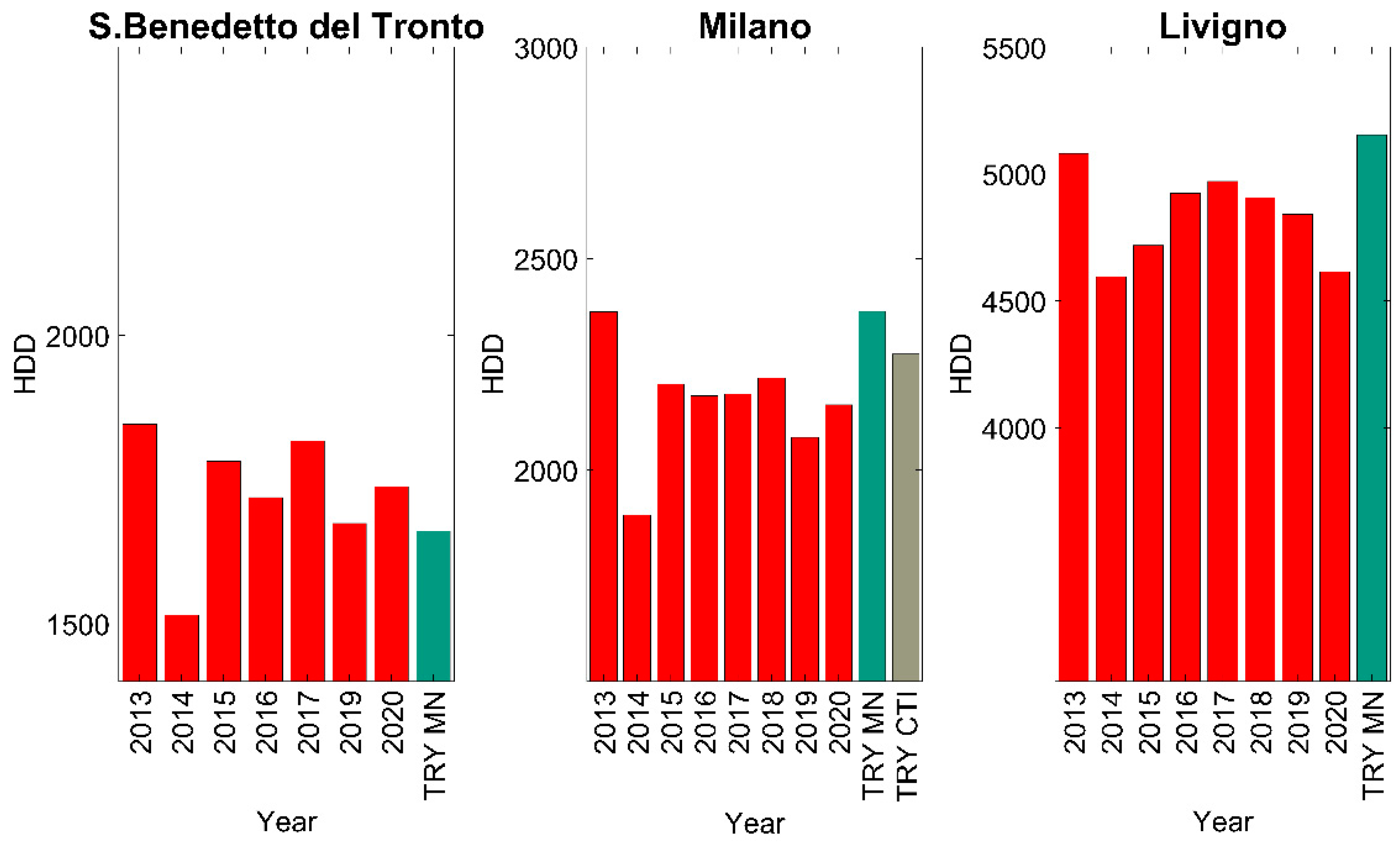
For all of the considered years, the values of the real heating degree days (HDD) are determined for each location, as shown in Figure 1, considering a reference temperature for its definition of 20 °C (according to DPR 412/93) and the reference period as prescribed by the UNI 11300/1 norm (from 15 October to 15 April for Milan, from 1 November to 15 April for San Benedetto del Tronto, and from 5 October to 22 April for Livigno). This figure shows important variation in HDD from a year to another for all of the towns considered. For example, if we focus our attention on San Benedetto del Tronto, the maximum value is 1846 for the year 2013, and the minimum value is 1515 for the year 2014, corresponding to an increase of 11% and a decrease of 9% with respect to the standard TRY value, respectively.

2.2. Building

In order to present general results that have not been influenced by the characteristics of a specific building, a building derived from the reference building proposed by IEA [24] was considered in this work. The simulated building was a two-floor family house characterized by a space heating demand of 45 kWh/m²y in the standard climate of Strasburg. The total floor area of the building considered in the simulations was 360 m², and the main building envelope thermal properties are presented in

Table 2. Geometrical and thermo-physical data of the building envelope components. [25].

Envelope Component	Thickness (m)	U-Value (W/m2K)
Ground floor	0.385	0.241
Floor	0.185	0.235
Roof	0.285	0.694
Internal wall	0.200	0.885
External wall	0.318	0.364

; in Figure 2, the 3D model of the building is sketched.

The air change rate due to infiltration was considered to be 0.3 h⁻¹ for all of the thermal zones, and all of the windows were double pane characterized by a 4-16-4 mm construction and were filled with Argon gas. The frame was 15% of the total area of the window (total area of the glass and frame), and the overall transmittance of the window was U-window = 1.5 W/m²K. The window arrangement is shown in

Table 3. Window arrangements of the considered building.

Orientation	Total Windows Area (m2)
North	14
East	20
West	20
South	30

.

Gains due to inhabitants and thermal gains caused by electric equipment were considered variable during the day, as shown in Figure 3. The thermal gain caused by a single inhabitant was divided in two parts: 20 W was considered the convective part of the thermal gain, and 40 W was the radiative part. The thermal gains due to electrical equipment were subdivided in half between the convective and radiative parts instead. For any parameter not explicitly mentioned in this section, the value proposed by IEA Task 44 for SFH45 was employed and not was not explicitly reported here for the sake of brevity [24].

Obviously, the building considered in this study hasa different thermal load, depending on its location. In

Table 4. Design temperature t_des of the three towns and design thermal load P_th,des of the HP at design temperature.

Town	tdes (°C)	Pth,des (kW)
S. Benedetto del Tronto	−1	6.2
Milan	−5	7.9
Livigno	−19	13.9

, the building design thermal load is reported as a function of the design temperature of the different locations.

In the present paper, the software package TRNSYS was used to model the building, and in particular, the multizone building TRNSYS type 56 [26,27].

2.3. Heat Pumps

A total of three different inverter ASHPs (Unit 1, 2, and 3) were investigated. Unit 1 was coupled to the building placed in San Benedetto del Tronto, Unit 2 and Unit 3 were couples to the buildings located in Milan and in Livigno, respectively. The three heat pumps were characterized by the same coefficient of performance (COP) values, represented in Figure 4 as a function of outdoor air temperature and for different compressor inverter frequencies. The modulation range of the inverter was between 23 Hz and 90 Hz. On the other hand, the thermal power supplied by the three heat pumps was different. In fact, the considered units were sized to totally match the thermal energy demand of the building to which the pumps were coupled. In Figure 5, the building energy signature (black line) is shown together with the thermal power supplied by the three heat pumps at the maximum frequency, 90 Hz. Moreover, it is evident from that figure how the bivalent temperatures for the three HPs were equal to the design temperatures presented in Table 4.

2.4. Heating System

In Figure 6, a sketch of the heating system layout is represented. The building is characterized by two thermal zones, one for each floor. The heating system presents a thermal storage of 0.2 m³ (the same for all the scenarios considered) and three-speed fan-coils as emitters (one fan-coil for each zone, characterized by different power to supply the correct thermal energy). Each terminal unit is characterized by an on-board controller, which selects the fan speed on the basis of indoor air temperature. The set-point temperature for the indoor air is 20 °C along the whole heating season.

3. The Modelization of Frosting and Defrosting Cycles and Heat Pump Performance

In this paper, reverse-cycle defrosting (RCD) was considered to melt the ice that is unavoidably deposited on the evaporator. In fact, among the many solutions to melt the ice build-up on the evaporator, RCD is the most widespread methodology adopted by commercial air-to-water heat pumps [28]. During the defrosting transient, the heat pump reverses the thermodynamic cycle and transfers the heat from the building to the external finned heat exchanger. It is important to stress how, in this case, the water thermal storage installed within the heating system allows the mitigation of the negative impact of the defrost cycles on indoor comfort conditions. In fact, thermal energy can be drawn from this element, avoiding a noticeable decrease in internal air temperature.

As highlighted by the literature, there are many possible control logics of defrost cycles. In particular, the defrosting technique (e.g., RCD, hot-gas bypass, water spray, electric heating), the duration of defrost cycle, and the algorithm to start defrosting are elements that have been deeply investigated by researchers and heat pump manufacturers [13,28,29].

In this analysis, we considered a constant pump cycle duration that was equal to 5 min [30] with a constant electric power absorbed by the heat pump and a constant thermal power drawn by the tank during the whole defrost cycle. A simple model for establishing when the heat pump needed defrosting was introduced. The evaporator of the machine was considered as a black box (an open thermodynamic system), as shown in Figure 7. The air stream entered the evaporator in conditions expressed by Subscript 1 and exited in the conditions expressed by Subscript 2. The term m_w (kg/s) represents the mass flow rate of water condensed on the heat exchanger that may freeze. The symbol t refers to the temperature, x refers to the vapor quality, and h refers to the specific enthalpy of the air stream. All of the parameters associated with Entry State 1 are known since they refer to the conditions of the outdoor ambient air. Using the psychrometric formula proposed by [31]:

$$\mathrm{h}=1.006\mathrm{t}+\mathrm{x}\left(2501+1.84\mathrm{t}\right),$$

(3)

the enthalpy h₁ (kJ/kg) as well as the dew point temperature t_DP (°C) can be calculated and given by

$${\mathrm{t}}_{\mathrm{DP}}=\frac{4030.183}{16.6536-\ln \left(\frac{{\mathrm{p}}_{\mathrm{sat}}}{1000}\right)}-235,$$

(4)

$${\mathrm{p}}_{\mathrm{sat}}=1000\exp \left(16.6536-\frac{4030.183}{\mathrm{t}+235}\right)$$

(5)

where p_sat (Pa) is the saturation vapor pressure of the water vapor available in the air at the conditions expressed by Subscript 1. The vapor quality of the mixture at the dew point can be calculated as well, by means of the relation

$${\mathrm{x}}_{\mathrm{DP}}=0.622\frac{{\mathsf{\phi }\mathrm{p}}_{\mathrm{sat}}}{{\mathrm{p}}_{\mathrm{tot}}-{\mathsf{\phi }\mathrm{p}}_{\mathrm{sat}}},$$

(6)

where φ is the relative humidity (in this case φ = 1) and p_tot (Pa) is the atmospheric pressure at the altitude of the selected location.

Equations (4) and (6) allow the air enthalpy at the dew point to be obtained, namely

$${\mathrm{h}}_{\mathrm{DP}}=1.006{\mathrm{t}}_{\mathrm{DP}}+{\mathrm{x}}_{\mathrm{DP}}\left(2501+1.84{\mathrm{t}}_{\mathrm{DP}}\right).$$

(7)

The air enthalpy at the dew point gives information about the moisture formation (and subsequently, the possible frost formation) on the evaporator of the heat pump: if the air enthalpy at the outdoor heat exchanger outlet in Condition 2 is lower than h_DP, frost formation on the heat exchanger may occur, and the defrost cycle has to start after a certain interval. The enthalpy h₂ of the air stream at the outlet of the evaporator can be calculated approximately (neglecting the enthalpy of the of the water that condenses on the finned coil) by applying an energy balance to the heat exchanger:

$${\mathrm{h}}_2={\mathrm{h}}_1-\frac{{\mathrm{Q}}_{\mathrm{ev}}}{{\mathrm{m}}_{\mathrm{a}}},$$

(8)

where Q_ev (kW) is the thermal power exchanged with the outdoor air by the machine’s evaporator, and m_a (kg/s) is the air mass flow rate exiting the evaporator (also, in this case, the air mass flow rate exiting the evaporator is the same the one that enters the heat exchanger whenever the mass of water condensed on the evaporator may be neglected). Typically, the quantity of air processed by a heat pump is a parameter given in the technical datasheet of the unit, and the term Q_ev can be calculated applying an energy balance to the whole heat pump. In fact, the unit works by extracting the power Q_ev from the evaporator, thus providing the thermal power P_th to the condenser and absorbing the electric power P_el. Hence

$${\mathrm{Q}}_{\mathrm{ev}}={\mathrm{P}}_{\mathrm{th}}\left(1-\frac{1}{\mathrm{COP}}\right),$$

(9)

where COP is the coefficient of performance of the HP, defined as the ratio between thermal power P_th and electric power P_el.

This simple model of a RCD can be easily implemented in TRNSYS with no additional data on the heat pump evaporator, using only technical data from the heat pump datasheet.

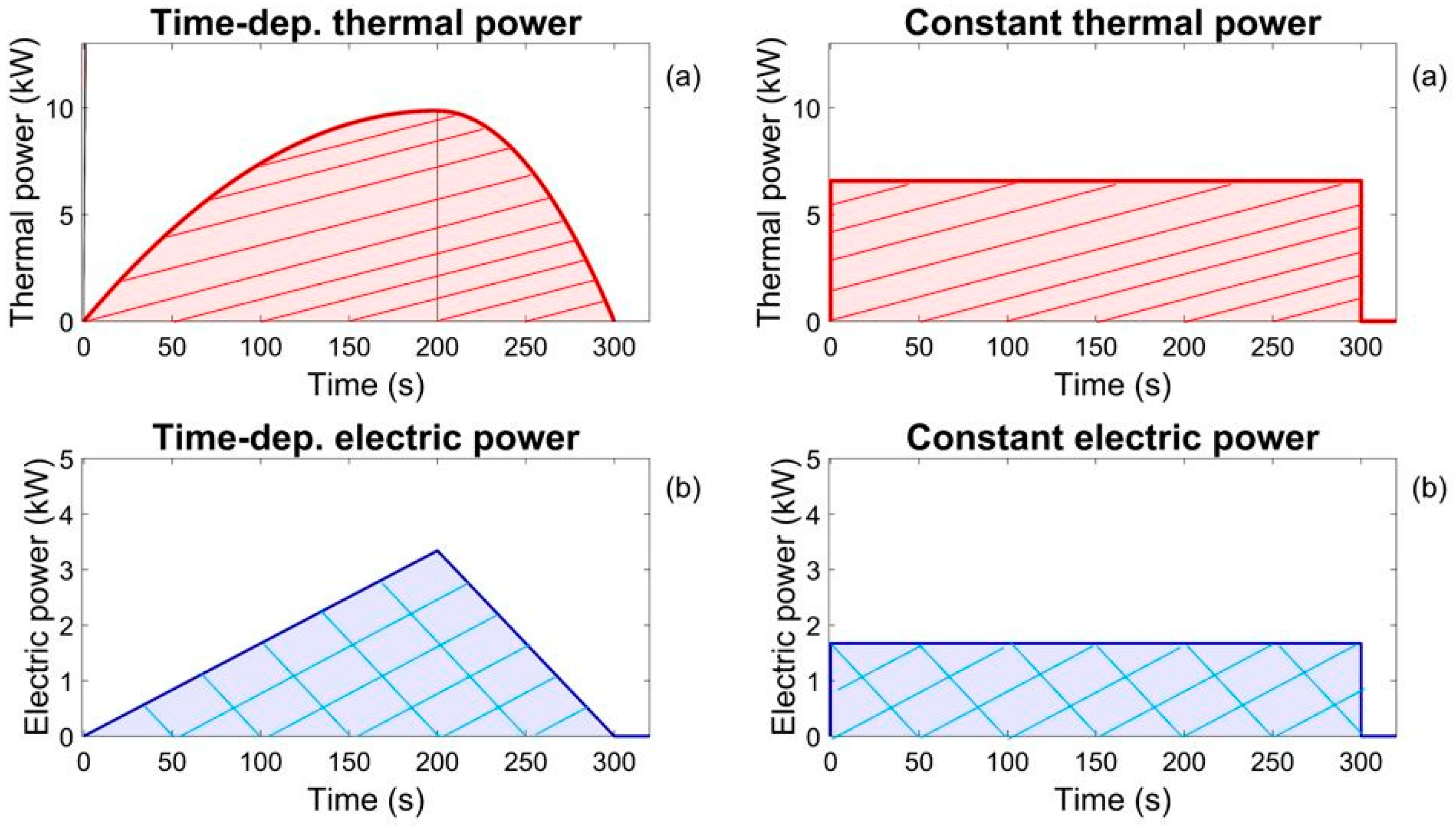
In [11], the authors simulated the RCD using time-dependent functions for electric and thermal power during the defrosting phase; a similar analysis can only be made if a huge amount of data are available from the manufacturer or if long-term experiments are conducted on a specific heat pump. Referring to the three heat pumps that are be investigated in this paper, the electric power input of the heat pump and the thermal power taken from the water tank are considered as constants along the defrost cycle. Their values are shown in

Table 5. Thermal power drawn from the building by the heat pump during a defrost cycle, P_th,def, electric power absorbed by the machine during defrost, P_el,def, and air mass, m_a, processed by the evaporator of the machine.

Heat Pump	Pth,def (kW)	Pel,def (kW)	ma (kg/s)
Unit 1	4.59	1.17	1.65
Unit 2	6.57	1.67	2.11
Unit 3	15.68	3.99	4.22

. Furthermore, additional details on the choice of both the values for the electric power and the thermal power are given in Figure 8. In detail, we assume for the same energy for the whole defrost cycle as well as the same electric energy input for each different HP, as proposed in [11]. In particular, the thermal and electric power trends along a generic defrost cycle are reported in Figure 8, according to the model proposed in [11]. The thermal power trend is modelled with two parabolic branches, while the electric power is modeled with two linear functions. In the same figure, the thermal and electric power considered in this analysis are reported, i.e., two constant functions during the whole defrost cycle of 300 s. In Figure 8, the surfaces below the lines are equal to both, with reference to the thermal power (a) and to the electric power (b). Moreover, the duration of the defrost cycle is taken as in [11] and corresponds to a mean time used by the manufacturers on their control systems.

The air mass processed by the heat pumps is assumed to be a linearly increasing function of the thermal power of the machine, according to data given by a manufacturer [32]: used data refer to heat pumps characterized by a nominal thermal power ranging from 4.7 kW to 31 kW. The values of the air mass processed by the three HPs considered are presented in Table 5 and were obtained applying a linear interpolation on the abovementioned data given by the HPs’ manufacturers.

In Figure 9, the defrost control implemented in TRNSYS is shown through a flowchart diagram. It can be noticed that the defrost phase only starts if two conditions are simultaneously satisfied: (1) the enthalpy of the air at evaporator outlet is lower than the enthalpy at the dew point; (2) the HP is turned on.

Annual simulations were conducted, as in [10], considering the same building and the different heat pumps described in previous sections. Since the three considered municipalities are located in different climatic zones, the operating period of the heating system was assumed to be the standard period corresponding to each climatic zone, as explained in Table 1. In all of the simulations, a water supply temperature from the heat pump of 45 °C was assumed, a typical set-point temperature for fan-coil applications.

First, for each location and each year, a simulation was conducted, neglecting the influence of HP defrost. Then, further simulations were conducted with reference to the same years and locations, assuming the presence of defrost cycles, as shown in the previous section of this chapter. In all of the simulations, a time step of 30 s was considered.

The analysis allowed the evaluation of the seasonal coefficient of performance, SCOP, defined as

$$\mathrm{SCOP}=\frac{\mathrm{ET}}{{\mathrm{EE}}_{\mathrm{HP}}+{\mathrm{EE}}_{\mathrm{DEF}}}$$

(10)

where EE_HP (kWh) is the total electrical energy absorbed by the heat pump along the heating season, EE_DEF (kWh) is the seasonal electrical energy input of the HP during the defrost cycles, and ET (kWh) is the thermal energy globally supplied by the heat pump to the plant during the season.

4. Results and Discussion

In Figure 10, the number of defrost cycles are reported for every year considered in the simulations. The HP placed in Milan performs more defrost cycles than the units placed in Livigno and San Benedetto del Tronto. It can be observed that there is an important variability in the number of defrost cycles conducted from a year to another for all of the towns considered, and we should also indicate that the test reference year generally underestimates the number of defrost cycles performed by the units, as noted in

Table 6. Maximum, minimum, and TRY number of defrost cycles.

Location	Maximum	Minimum	TRY
Milan	1595 (year2018)	827 (year 2015)	802 (CTI TRI)
Livigno	1008 (year 2019)	254 (year 2013)	340
San Benedetto del Tronto	904 (year 2013)	235 (year 2019)	158

.

In Figure 11 the thermal energy demand of the building and the seasonal coefficient of performance as defined in Equation (10) are reported for different years and municipalities. The figure shows that for every considered case, the thermal energy demand is always higher when defrost is taken into account with respect to the case of negligible defrosting; on the contrary, the SCOP is lower when defrosting is taken into account.

The variation in thermal energy demand from a year to another is relevant for all of the investigated municipalities: in particular, focusing on simulations that consider defrosting and refer to San Benedetto del Tronto, the thermal energy demand for 2013 is 6009 kWh, almost two times the thermal energy demand of 2020, which is equal to 3184 kWh. On the contrary, the seasonal coefficient of performance displays smaller variations from one year to another. In detail, in the defrost case, the SCOP assumes values in the range 2.86–2.99, with mean value 2.93; indeed, the percentage changes referring to the mean value are 2.4%/+2%. By neglecting the defrost cycles, the SCOP assumes values in the range 3.01–3.21, a displaying mean value 3.09 and percentage changes with respect to the mean value −2.8%/+3.6%.

Concerning the test reference year defined through Meteonorm for San Benedetto del Tronto, the thermal energy demand of the building is overestimated in both cases, with or without defrost (thermal energy demand is lower with respect to the TRY predictions for 5 years out of 7); conversely, SCOP values obtained from the test reference year are in accordance with the values obtained from the simulations that considered real weather data from the different years.

Considering Milan, Figure 11 shows, as for the case of San Benedetto del Tronto, important variations of the thermal energy demand from one year to another (considering defrost, minimum value of 9257 kWh for 2019 and maximum value of 14,009 kWh for 2013; neglecting defrost, minimum value of 8676 kWh for year 2019 and maximum value of 13316 kWh for year 2013). Slight fluctuations in the SCOP value are obtained, but these variations are smaller than in the case of San Benedetto del Tronto (defrost case SCOP range 2.72–2.83, neglecting defrost SCOP range is 2.84–2.94). Similar results are obtained for Livigno, with important variations in thermal energy from a year to another (range for defrost case 30,329 kWh–36,183 kWh, range neglecting defrost 29,496 kWh–35,685 kWh). In fact, for Livigno, sensible variations in the SCOP values (up to 5.6%, referring to SCOP mean value of the years 2013–2020) that are higher than for San Benedetto and for Milan (range for defrost case 2.46–2.71 range neglecting defrost 2.5–2.79) are achieved.

Figure 11 as also shows that the Meteonorm TRY for Livigno underestimates the thermal energy demand as well as the SCOP value. On the other hand, the Meteonorm test reference year for Milan generally overestimates the thermal energy, while the SCOP values are similar to those obtained using real weather data. Moreover, in the special case of Milan, CTI TRY seems to be more reliable than Meteonorm.

Generally speaking, the TRY understimates the number of defrost cycles. In detail, it underestimates the number of yearly hours when defrost may occur, i.e., when the couple temperature–relative humidity assumes values such that frosting at the evaporator may occur.

Finally, another aspect that can be observed from Figure 11 is the percentage increase in the thermal energy demand considering the case with defrost respect to the case that neglects defrost for the same year: it is evident how, for Milan, the building needs more thermal energy, up to +7.9% (year 2020), than for San Benedetto del Tronto (maximum increase of 5.5% for year 2014) and for Livigno (maximum increase of 4% for year 2019). These results are in agreement with those of other researchers ([31]), confirming the significant influence of energy losses linked to defrost cycles on the heat pump SCOP.

In Figure 12, the electrical energy absorbed by the HP for all of the simulations performed is reported together with the percentage increase of electrical energy consumption considering defrost respect to the case with no defrost for every year. It can be observed that the percentage increase is higher for Milan (mean value +10.7%) and San Benedetto del Tronto (mean value +9.5%) than for Livigno (mean value +4.6%).

5. Conclusions

In this paper, dynamic simulations of the seasonal coefficient of performance SCOP of ASHPs have been presented. Simulations were conducted by employing the software package TRNSYS and by investigating three different heat pump systems coupled with the same building located in three different Italian municipalities: S. Benedetto del Tronto (Central Italy, 42°58′ North, 13°53′ East), Milan (North of Italy, 45°28′ North, 9°10′ East), and Livigno (North of Italy, 46°28′ North, 10°8′ East). Real weather data (i.e., outdoor air temperature and humidity as well as solar radiation) available for the three abovementioned cities for a period of 8 years (2013–2020) were introduced within numerical models, and a comparison with the standard test reference year for each location was conducted as well. Attention was paid to the modeling of defrost cycles in order to evaluate its influence on the heat pump SCOP. The main outcomes of the obtained simulations can be summarised as follows:

• Referring to different years, the thermal energy demand displays huge variations (in some cases it can even double its value);
• On the contrary, the SCOP displays small variations with respect to its mean value. SCOP also displays small variations considering defrost vs. no defrost cases (

  Table 7. Maximum and mean SCOP decrease considering defrost vs. no defrost cases; obtained from the dynamic simulations considering real climatic data.

  Location	Maximum Decrease	Mean Decrease
  Milan	5.2%	4.1%
  Livigno	3.4%	1.9%
  San Benedetto del Tronto	9%	5.4%

  );
• SCOP values obtained from the test reference year often tend to overestimate or underestimate the SCOP value, and in the special case of Milan, CTI TRY seems to be more reliable than Meteonorm;
• The electrical energy absorbed by the HP considering defrost is higher with respect to the case with no defrost for every year; it can be observed that the percentage increase is higher for Milan (mean value +10.7%) and San Benedetto del Tronto (mean value +9.5%) than for Livigno (mean value 4.6%). Indeed, if one neglects the effect of defrosting, there is a tendency to underestimate the electric energy consumption of the HP up to 10%.

To sum up, frosting/defrosting cycles have to be taken into account in order to correctly evaluate the electric energy consumption of a HP. The use of TRY instead of real data tends to underestimate the number of defrosting cycles, and a revision of TRY should help manufacturers and technicians.