Scattering Evaluation of Equivalent Surface Impedances of Acoustic Metamaterials in Large FDTD Volumes Using RLC Circuit Modelling

Abstract

Most simulations involving metamaterials often require complex physics to be solved through refined meshing grids. However, it can prove challenging to simulate the effect of local physical conditions created by said metamaterials into much wider computing sceneries due to the increased meshing load. We thus present in this work a framework for simulating complex structures with detailed geometries, such as metamaterials, into large Finite-Difference Time-Domain (FDTD) computing environments by reducing them to their equivalent surface impedance represented by a parallel-series RLC circuit. This reduction helps to simplify the physics involved as well as drastically reducing the meshing load of the model and the implicit calculation time. Here, an emphasis is made on scattering comparisons between an acoustic metamaterial and its equivalent surface impedance through analytical and numerical methods. Additionally, the problem of fitting RLC parameters to complex impedance data obtained from transfer matrix models is herein solved using a novel approach based on zero crossings of admittance phase derivatives. Despite the simplification process, the proposed framework achieves good overall results with respect to the original acoustic scatterer while ensuring relatively short simulation times over a vast range of frequencies.

1. Introduction

Over recent decades, there has been a lot of progress regarding numerical simulation techniques in the field of wave physics, mostly benefiting from modern hardware and software improvements. However, computing limits can still be reached in most frequency- or time-domain numerical problems. Both approaches come with their own strategies for approximating wave equations within a bounded space. Usually, the accuracy and computational time of such schemes are dependent on the minimal size of the meshing grid, on the hardware at hand, the frequency to be studied, and on the overall size of the numerical environment. To a relative degree, numerical schemes tend to be computationally cheaper for modelling either complex geometries in small spaces or simpler geometries within larger spaces. The suitability of one method over the other generally depends on the scope of the study.

There are cases, however, where simulations of complex geometries in larger sceneries are of specific interest, i.e., sceneries where intricate geometry with fine meshing is required at a local scale, but the physical effect of such geometry must be studied within a much more global environment. An example of such a study can be found in simulations involving metamaterials, which are usually quite compact, where their influence over a larger three-dimensional context may be of interest. Metamaterials are composite structures engineered in such a way that they can display extraordinary physical properties within deep-subwavelength dimensions, i.e., dimensions much smaller than the design wavelength. As such, metamaterials come in a variety of shapes for many wave-control applications, going from frequency-selective structures for cloaking [1] or trapping [2] to reconfigurable radiation patterns for imaging [3] and telecommunications [4], with scales ranging from optical [5] to seismic [6] wavelengths, passing through microwave [7], ultrasound [8] and audio frequencies [9]. In the case where the volume of the simulated scenery happens to be very large compared to the metamaterial meshing dimensions, traditional modelling strategies could prove non-viable within realistic means, likely resulting in immense computational times and memory requirements. This calls for alternative strategies in modelling local wave interactions at boundaries and their respective propagation behaviour in much larger spaces within more reasonable computational means.

This problematic has sprung a rising number of research initiatives for many decades. The concept of impedance [10] has helped in establishing a strategy for approximating the physical conditions created by the geometry of an object by a set of impedance boundary conditions (IBC) [11]. Many of such investigations began to appear in numerical applications linked to electro-magnetic [12,13], heating [14], and acoustic [15] problems to reduce the computational load, particularly so in the early years of scientific computer simulations. Lately, this strategy has seen multiple uses for simplifying intricate subwavelength structures, such as metamaterials [16,17,18,19]. On top of analytical impedance approximations, the Resistor-Inductor-Capacitor (RLC) circuit impedance analogy between electrical and mechanical systems [10] has also allowed for simpler expressions of resonant structures. This becomes notably useful for the description of metamaterials made of locally resonant elements [20]. In the context of large-scale acoustic computation, time-domain methods offer the advantage to simulate a vast range of frequencies for large spaces in a single computation run [21]. Many of the works in this field emphasise the use of frequency-dependent boundary conditions to describe the acoustic characteristics of the interfaces present in the model [22,23,24,25,26,27,28,29]. However, to the authors knowledge, no work has yet been conducted for applying metamaterial-based impedance boundary conditions into large-scale time-domain acoustic computational methods.

In this work, we propose an acoustic scattering study where compact metamaterial-inspired acoustic diffusers, called metadiffusers [30,31,32], are considered too complex to simulate directly in a 3D Finite-Difference Time-Domain (FDTD) scheme, and thus decide to evaluate the computational and scattering impact of RLC IBCs on the diffuse field of a larger space in which they could be installed, such as an orchestra pit. Figure 1 illustrates this approach, where the scaled scheme of a $N=5$ slits Quadratic Residue Metadiffuser (QRM) used here as a reference compact metamaterial is shown in Figure 1a. The local scattering generated by the metadiffuser can be alternatively reproduced through a simplification of the metamaterial geometry into a set of IBCs. The resulting IBCs can thereafter be reproduced through an RLC circuit [28] integrated at the desired boundaries of the 3D FDTD volume, as illustrated in Figure 1b,c. The novelty of this approach lies in the optimised fitting of the RLC circuit IBCs based on zero crossings of admittance phase derivatives in order to ultimately replicate the scattering generated by metamaterial structures in large FDTD volumes. A time-domain scheme has been chosen for this work as not only it can wield broadband frequency information, but also enables time-domain signal processing which can later be used for further virtual audio operations for auralisation and spatialisation purposes.

2. Theoretical Modelling

Acoustic scattering occurs when a travelling sound wave encounters an obstacle or inhomogeneity in its path, e.g., a solid object or a change of medium density, and thus breaks into secondary spreads out from it in a variety of directions. The magnitudes and directions of such scattered waves can be described by the Helmholtz–Kirchhoff theory of diffraction, which uses Green’s theorem to determine the scattered pressure at any given point by specifying the wave field onto the scattering obstacle. However, the latter formulation is generally approximated depending of contextual assumptions regarding the distance of the source and observer from the scattering object compared to the monochromatic wavelength. This leads to two major situations, i.e., (i) the near-field where the source and observer are relatively close to the obstacle, under the Rayleigh critical distance ($R_0=S/\lambda$, where S is the area of the surface and $\lambda$ the wavelength of the wave), and (ii) the far-field where the source and observer are considered to be far away from the obstacle, in the limit of infinity.

On a first instance, we will focus on the frequency-dependent scattering made by the metasurface, where the acoustic field at a point $\mathbf{r}=\mathbf{r}(x,y,z)$ scattered by a surface centred at ${\mathbf{r}}_0=\mathbf{r}(x,y,z=0)$ can be approximated by the Rayleigh-Sommerfeld integral as

$$P_s\left(\mathbf{r}\right)=-i\frac{k}{2\pi }{\int }_{S_0}\frac{p_0\left({\mathbf{r}}_0\right)R\left({\mathbf{r}}_0\right)e^{ik\mid \mathbf{r}-{\mathbf{r}}_0\mid }}{\mid \mathbf{r}-{\mathbf{r}}_0\mid }\mathrm{d}S,$$

(1)

where $p_0\left({\mathbf{r}}_0\right)$ is the incident pressure field, and $R\left({\mathbf{r}}_0\right)$ is the spatially dependent reflection coefficient of the locally reacting surface $S_0$, with $k=\omega /c_0$ being the wavenumber in air at the angular frequency $\omega$ and speed of sound $c_0$. Here, the Fourier transform of $f\left(x\right)$ is $\widehat{f}\left(k\right)$, which is given by $\widehat{f}\left(k\right)=\int f\left(x\right)e^{-ikx}\mathrm{d}x$. It transpires from Equation (1) that defining the state of the spatially dependent reflection coefficient, $R\left({\mathbf{r}}_0\right)$, is ultimately important to determine the directions and magnitudes of the scattered sound energy. In the case of metadiffusers, the spatially dependent surface reflection coefficient is obtained through the Transfer Matrix Method [30] (TMM), which relates the acoustic pressures and normal particle velocities at the extremities of a one-dimensional acoustic system; here, a slit loaded with Helmholtz resonators (HRs). The surface reflection coefficient and characteristic impedance of the n-th slit, $R_{slit}^n$ and $Z_{slit}^n$, respectively, can be interchangeably deduced one from the other by the relation

$$Z_{slit}^n=Z_0\frac{1+R_{slit}^n}{1-R_{slit}^n},$$

(2)

where $Z_0={\rho }_0{c}_0$ is the characteristic impedance of air.

The diffusion coefficient of a surface rates the uniformity of the aforementioned scattered sound field. Moving to a spherical coordinate system where $P_s\left(\mathbf{r}\right)=P_s(\theta ,\varphi ,r)$ with $\theta$ and $\varphi$ being the elevational and azimuthal planes respectively and r being the distance to the origin, the directional diffusion coefficient [33], ${\delta }_{\psi }$, produced when a sound diffuser is radiated by a plane wave at the incident angle $\psi =({\theta }^{\prime },{\varphi }^{\prime })$ (primed superscripts denoting incident angles), can be estimated from the hemispherical autocorrelation of the scattered distribution

$${\displaystyle {\delta }_{\psi }=\frac{{\displaystyle {\left[{\displaystyle \int \int I_s(\theta ,\varphi )\mathrm{d}S}\right]}^2-\int \int I_s^2(\theta ,\varphi )\mathrm{d}S}}{{\displaystyle \int \int I_s^2(\theta ,\varphi )\mathrm{d}S}},}$$

(3)

where $I_s(\theta ,\varphi )\propto {\left|p_s(\theta ,\varphi )\right|}^2$ is proportional to the scattered intensity. The integration is performed over a hemispherical surface ($-\pi /2\le \theta \le \pi /2$ and $0<\varphi <2\pi$) where $\mathrm{d}S=\mathrm{d}\theta \mathrm{d}\varphi$. This coefficient must be normalised to that of a plane reflector, ${\delta }_{flat}$, to eliminate the diffracting effect caused by the finite size of the structure, i.e., ${\delta }_{n,\psi }=({\delta }_{\psi }-{\delta }_{flat})/(1-{\delta }_{flat})$. In this works we analyse the 3D case of a normal incident wave, i.e., $({\theta }^{\prime },{\varphi }^{\prime })=(0,0)$ and ${\delta }_{n,\psi }\equiv {\delta }_{n,0}$.

3. RLC Circuit Impedance Boundary Formulation

The magnitude and phase of the surface impedance of a metadiffuser are marked by the inherent resonances of the structure, i.e., if it has one or more resonators it should show one or more fundamental resonant peaks or phase shifts in its surface impedance. In the case of the QRM, a highly resonant structure with two HRs per slit is displayed, which lends itself to a boundary formulation based on a combination of second-order resonators. Example admittances for two slits of the QRM are shown in Figure 2. The two slits displayed in Figure 2 are both loaded with two HRs but with different slit and HR dimensions. This results in different surface impedances for each slit, thus presenting different resonance peak amplitudes and phase shifts.

One useful passive formulation for a given slit impedance consists of a parallel set of series RLC circuits (after [28]), each consisting of one resistor (R), one inductor (L) and one capacitor (C), where all RLC parameters are non-negative and real-valued. The admittance of this structure in the Laplace domain is given by

$$Y\left(s\right)=\sum _{b=1}^B\frac{1}{Z^{\left(b\right)}},Z^{\left(b\right)}=L^{\left(b\right)}s+{\mathbf{r}}^{\left(b\right)}+1/\left(s{C}^{\left(b\right)}\right),$$

(4)

where $L^{\left(b\right)}$, $R^{\left(b\right)}$, and $C^{\left(b\right)}$ are non-negative constants for each branch. For our analyses and optimisations, we can limit s to $s=j\omega$, and where $B\ge 1$ is the number of RLC branches. The associated impedance of the RLC circuit is then simply $Z\left(j\omega \right)=1/Y\left(j\omega \right)$. With this impedance boundary formulation we aim to fit the surface impedance of each slit of the QRM with an equivalent circuit made up of a set of resonances with non-negative RLC parameters. The passivity of this structure is then preserved in the discrete FDTD setting through the choice of the bilinear transform as a discretisation method [34]. This impedance model can be seen as an extension of various simpler frequency-dependent boundary models presented in the context of FDTD methods for room acoustics [35,36,37].

A methodology for fitting RLC parameters is described in [28], which consists of: (i) identifying resonances in an admittance by their peaks in the admittance magnitude, and (ii) estimating half-power bandwidths for each resonance from admittance magnitude. From those estimates RLC parameters may be identified for each resonance. This is followed by a global optimisation over the RLC triplet parameters using a Nelder–Mead optimisation. That approach works well when admittance peaks are well-separated, but in general peaks in admittance magnitude data can be difficult to identify, and furthermore half-power bandwidths can be hard to estimate from admittance magnitude data alone. This is especially true in the example admittances shown in Figure 2. Other ways for approximating the weight and resonant frequencies in viscoacoustic problems were also previously reported [38].

In this study, we use an approach which is based on making use of admittance phase information, and derivatives thereof, to identify resonance parameters. It can be observed from Figure 2 that peaks in admittance magnitude are linked to inversions in the phase response. More specifically, we know that the phase response of an individual-series RLC circuit admittance goes to zero at its resonant frequency and displays a negative slope at that frequency. Additionally, regarding the slope of the phase at the resonant frequency, one can derive from Equation (4)

$$-{\left.\frac{\partial \angle Y\left(i\omega \right)}{\partial \omega }\right|}_{\omega ={\omega }_0}=\frac{2}{\mathrm{\Delta }\omega }=\frac{2L}{R},$$

(5)

where ${\omega }_0=1/\sqrt{LC}$. Thus, after detecting a resonance in the admittance phase from its slope and zero crossings, and after sampling the associated peak in the admittance magnitude, the half-power bandwidth, $\mathrm{\Delta }\omega$, follows from Equation (5) (which may be estimated with simple finite differences). This approach is sufficient to obtain RLC parameters for each well-isolated resonance, and can be more robust than peak detection and half-power bandwidth estimation from the admittance magnitude alone. Nevertheless, this approach still has limitations for very-closely spaced resonances (examples can be seen in Figure 2) where the phase response at a resonance may not cross zero (and thus would not be detected with this approach so far). To deal with such issues, the second derivative of the phase is additionally used to identify resonances, which can be written as:

$${\left.\frac{{\partial }^2\angle Y\left(i\omega \right)}{\partial {\omega }^2}\right|}_{\omega ={\omega }_0^{\prime }}=0,{\omega }_0^{\prime }={\omega }_0\sqrt{\sqrt{4-{(\mathrm{\Delta }\omega /{\omega }_0)}^2}-1},$$

(6)

where ${\omega }_0^{\prime }$ is the angular frequency at which there is a zero crossing in the second-order derivative of the admittance phase. Furthermore, ${\omega }_0^{\prime }\approx {\omega }_0$ provided that ${(\mathrm{\Delta }\omega /{\omega }_0)}^2\ll 1$, which means that ${\omega }_0^{\prime }$ may be used as an initial estimate of ${\omega }_0$ to seed the subsequent global optimisation. Identified resonances using this phase-derivative zero-crossing method (grey dotted lines) can be seen in Figure 2.

Once a set of RLC triplet parameters has been identified given a set of resonant frequencies and associated bandwidths, a global optimisation using a Nelder–Mead method [39] as a non-linear minimisation algorithm is carried out to find the $L^{\left(b\right)}$, $R^{\left(b\right)}$ and $C^{\left(b\right)}$ that minimise $ϵ=\parallel Y_{TMM}-Y_{\mathbf{r}LC}\parallel$, where for a given slit, $Y_{TMM}$ is the target admittance output from the TMM model of the QRM, and $Y_{\mathbf{r}LC}$ is the impedance output of the RLC circuit. Fit reflection coefficients of the two QRM slits previously illustrated (see Figure 2) can be seen in Figure 3. It can be observed that this methodology is successful in capturing the resonances within the QRM slits. The errors shown take into account magnitude and phase, and discrepancies can be seen at the upper limit of our range of frequencies (e.g., a resonance being ignored). Such discrepancies may be attributed to viscothermal losses in the TMM model which cause deviations from ideal second-order resonances. These could be mitigated using pairs of RLC triplets for each identified resonance to allow for better optimised results, but this was not pursued as a compromise of accuracy and model complexity.

For later comparison purposes, a similar approach for modelling the equivalent surface impedance of the QRM is adopted in a Finite Element Method (FEM) study in COMSOL Multiphysics 5.3™, where the N = 5 impedance patches were modelled using built-in impedance boundary conditions with the complex impedance data obtained from the TMM model as input. The resulting scattering data between the QRM and the equivalent surface made of different RLC circuits is shown in the next section.

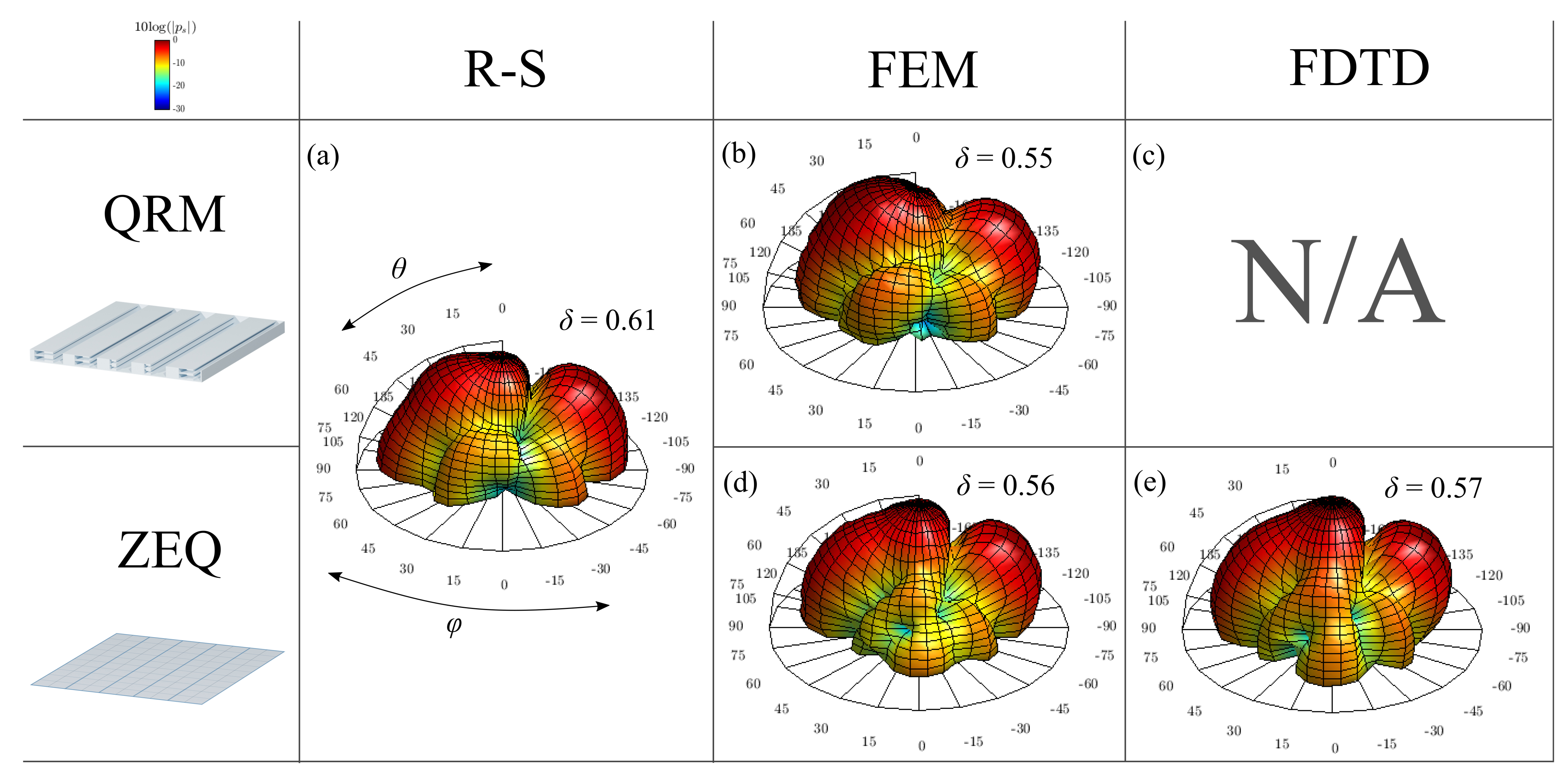
4. Spatial Acoustic Scattering

Figure 4 compares the 3D hemispherical scattered sound pressures of the aforementioned QRM with N = 5 slits and the equivalent RLC surface impedance, ZEQ, with N = 5 slits as well. The scattering distributions have been obtained through different methods, i.e., (i) the Rayleigh-Sommerfeld (R-S) integral for near-field scattering information, (ii) Finite Element Method (FEM) in COMSOL Multiphysics 5.3™, and (iii) Finite-Difference Time-Domain (FDTD) simulations. Numerical simulations in COMSOL were computed by installing the surface at the centre of a spherical domain filled with air, surrounded by a concentric perfectly matched layer (PML) with a far-field boundary condition at the boundary of the air domain to satisfy Sommerfeld’s radiation condition. A similar setup was used in the FDTD domain, but with first-order Engquist–Majda [40] absorbing boundary conditions at the boundary of a cubic air domain large enough to ignore any erroneous reflections in the obtained responses. The FDTD simulation was calibrated to have less than 1% numerical dispersion error up to 8 kHz with 10.5 points per wavelength (PPW) using the usual Courant-Friedrichs-Lewy (CFL) condition for the simplest 3D Cartesian scheme ($CFL=1/\sqrt{3}$), for which stability is ensured [21,41]. The time step, $T_s$, considered in the simulations can be deduced from the CFL condition as $T_s=X_s\times CFL/c$, where $X_s$ is the spatial sampling and c = 343 m/s is the speed of sound in air. Figure 4 shows the theoretical and numerical solutions of the surface scattered sound energy integrated over a radius distance of 1 m, so that all datasets represent a finite framework. In the FDTD model, virtual microphones were positioned at 1 m around the surface, which considering its edge dimensions (x, y) [35 cm, 35 cm], should be sufficient to correctly depict the scattered field at a frequency $f=2$ kHz. FEM results were obtained following a similar approach where the integration was performed over a spherical near-to-far-field boundary condition of 1 m radius.

Overall, the polar plots displayed in Figure 4a,b show some variations between the theory and FEM simulations, with normalised diffusion coefficient values varying from ${\delta }_{n,0}=0.61$ to ${\delta }_{n,0}=0.55$. These can be explained through the divergence of theoretical assumptions with respect to a numerical solving of the wave equation. More specifically, in a theoretical framework, the surface impedance is considered locally homogeneous for each slit, a fact that may not be entirely true in numerical terms due to the potential evanescent coupling between slits, a phenomenon not taken into account in the theory. As the scattered sound field is highly dependent on the distribution of the surface’s reflection coefficient, slight variations in the polar distributions can thus be expected. Nonetheless, it can be seen that the global shapes of the QRM sound scattering distributions are sensibly similar one to another, which can be confirmed by their close autocorrelation values. In addition, Figure 4b represents quite well the expected main dip that defines the Quadratic Residue sequence at $\theta \approx -{20}^{\circ }$ in the $\varphi =[-{90}^{\circ }:{90}^{\circ }$] elevation axis. The main axial and lateral energy lobes are also quite well represented. However, a slightly higher energy lobe can be discerned at $\theta ={20}^{\circ }$ in the FEM case. This is likely due to the finite size of the surface sample in the simulation, resulting in a decrease of the scattered sound energy at grazing angles, thus further relatively enhancing the remaining scattered energy and slightly reducing the intrinsic autocorrelation value. Despite such differences, the FEM model can be estimated to be in good agreement with the theoretical prediction.

The missing scattering distribution under Figure 4c is at the core of this work’s rationale, as it would be an unnecessarily complex task to simulate the fine features of the metadiffuser in a large 3D volume. The complex physics and the small geometry of the QRM not only would require an extremely fine meshing grid, and thus a very high computational load for conducting the same simulations, but viscothermal losses would have to be taken into account as well. This is why the aforementioned equivalent surface impedance as a fitted RLC circuit within an FDTD model is proposed to bypass the numerical limitations of large-scale multiphysics simulations, while faithfully reproducing the intended scattering of the metadiffuser embedded in a larger scene. It is worth noting that viscothermal losses inside the metasurface are implicitly encoded by the RLC approach in the FDTD scheme. However, in order to strengthen the forthcoming analysis between FEM and FDTD, scattering comparisons of a flat surface and a much simpler acoustic diffuser (e.g., a Quadratic Residue Diffuser) can be found in the Supplementary Materials, where excellent agreement between the different numerical methods can be observed.

Figure 4d shows the scattering distribution of the equivalent surface impedance simulated through FEM where the N = 5 impedance patches were modelled using impedance boundary conditions with input values identical to the analytical (TMM) surface impedance of the QRM. Again, it can be observed that the main dip at $\theta \approx -{20}^{\circ }$ is correctly reproduced, and that the main axial lobes are also in good agreement with the theory, leading to a normalised diffusion coefficient ${\delta }_{n,0}=0.56$ close to that of Figure 4b. The major changes that can be distinguished compared to the FEM simulation of the QRM are the energy distribution of the lateral lobes and the smoothing of the $\theta \approx {20}^{\circ }$ energy lobe. The former seems to resemble that of a flat panel scattering. Perhaps this is due to the disappearance of the slit cavities within each impedance patch which may cause variations from the estimated slit impedance values as these are dependent on the free air radiation correction of the slits. More investigation on that matter is needed.

Figure 4e similarly represents the scattered sound distribution of the ZEQ in the FDTD solver. Results are in excellent agreement with the ZEQ FEM data, with a very similar normalised diffusion coefficient ${\delta }_{n,0}=0.57$. A minor increase in scattered sound energy can however be perceived between FEM and FDTD ZEQ models which also appears in other cross-numerical comparisons that were conducted for traditional sound diffusers and flat surfaces (see Supplementary Materials). This slight energy increase in FDTD RLC modelling may then be attributed to energy propagation modelling in each numerical environment (FEM/FDTD), but remains nonetheless almost negligible with a difference in diffusion coefficient of 1%.

Although the equivalent surface impedance method proposed here results in a major simplification of the more intricate geometry of the metamaterial being studied, it can be seen that it is quite efficient for replicating an approximation of its scattered field into the surrounding space. Additionally, it has been previously shown that these FDTD simulations with such RLC circuit boundary conditions are amenable to parallel acceleration [29].

5. Temporal Acoustic Scattering

In addition to the previous spatial scattering results, a temporal acoustic scattering comparison is also here presented for evaluating the presence of time dispersion within the above-collected FDTD data. Figure 5 thus shows several wavelet transforms of scattered impulse responses corresponding to a flat panel, a traditional sound diffuser and the ZEQ. A fully modelled $N=5$ Quadratic Residue Diffuser (QRD) of dimensions [x, y, z](35, 35, 28) cm and design frequency $f_0=500$ Hz is here presented instead of a QRM due to the difficulty in modelling the latter structure in the FDTD solver. One must note that the QRM and QRD possess different scattering characteristics over the frequency range considered, only matching around 2 kHz.

Figure 5a shows the time-frequency information of the scattered impulse response captured at the top of a flat surface, at $z=1$ m. As expected, only a single hard reflection is obtained in the impulse response, covering the entirety of the frequency range of interest. A secondary reflection with much less intensity can also be identified, generated from the edge diffraction of the panel coming back to the receiver a couple of milliseconds after the first major reflection. This is supported by the inset displaying the time series of the reconstructed signal by inverse wavelet transform. Additionally, a late reflection with small amplitude can be observed at the end of the time window which may be due to spurious reflections not entirely absorbed by the surrounding Engquist–Majda absorbing boundary conditions.

The scattering obtained with the QRD via FDTD is illustrated in Figure 5b, where a strong temporal dispersion can be distinguished by the spreading of the scattered waves through time. In such figure, one can see a major reflection shortly followed by a similarly strong one, after which a series of multiple reflections appear with varying frequency content and continuously less energy. This provides with a good illustration of the scattering generated by the frequency-dependent behaviour of a sound diffuser. The blue dots represent the absence of frequency content in very narrow time periods. These are caused by wave interference due to the wavelength delay generated by the phase-grating diffuser, providing with a time-frequency dispersion pattern.

Ultimately, Figure 5c displays the scattered impulse response of the ZEQ obtained through RLC circuit filtering. It can be observed that a strong temporal dispersion is also obtained, with a similar pattern than the QRD. Even if the surface of the ZEQ is flat, it reproduces a similar frequency-dependent behaviour than a QRD—although, as mentioned previously, both temporal dispersions cannot be strictly compared one to the other. However, the scattering from the QRD serves as a good reference to observe the added temporal dispersion of the ZEQ.

6. Metadiffuser Equivalent Surface Impedance in a Large Space

For this work, an orchestra pit is chosen for a large scene in which to embed the proposed equivalent surface impedances in a 3D FDTD simulation. The geometry of the orchestra pit of general dimensions [x, y, z](8, 20, 2.5) is idealised as shown in Figure 6a, where a sound source S located at [x, y, z](2, 10, 1.5) and a receiver R located at [x, y, z](6, 10, 1.5) are highlighted. Note here that the pit is virtually isolated from the exterior environment of what would be the rest of an opera house. The considered orchestra pit is simulated following two different scattering strategies implemented on the walls. In the first situation, no particular scattering on the boundaries is considered, i.e., the walls are simply assumed perfectly rigid.

The FDTD simulation grid resolution was set to 10.5 PPW at 8 kHz, resulting in 4.8 billion computational elements, in order to obtain a numerical dispersion errors less than 1% [41] below such frequency. The simulations involving flat panels (no scatterers) required 30 GB of memory computed in parallel using Nvidia CUDA spread over four Nvidia Titan X GPU cards (Maxwell architecture). Simulations times with flat panels were approximately 55 min for 0.5 s of simulated response. Including the more complex RLC boundary conditions, the FDTD simulation took 65 min and required 3% more memory running on the same GPUs. Thus, the equivalent surface impedance incurs some extra minimal simulation costs (as expected from [29]), and it is also much smaller relative to the simulation costs expected for a full-fledged multiphysics simulation (taking into account QRM details and physics) in this space up to the chosen frequency resolution.

The impulse responses captured within this environment are analysed by means of a Spatial Decomposition Method (SDM) [42], which allows the determination of the directions of arrival (DOA) [43,44] of sound events in a 3D set of spatial impulse responses. The latter are captured through a microphone array and can be windowed over different integration times to show the evolution of the spatial sound field with respect to time. In this case, a $3\times 3\times 3$ virtual microphone array was used for recording the numerical impulse responses at the receiver location, and is displayed in Figure 6b. For data processing, the SDM Toolbox [45] made available by the Virtual Acoustics Team at Aalto University, Finland, was used. The impulse responses cover a frequency range ${\mathrm{\Delta }}_f$ = [20:8000] Hz and are integrated over several incrementing time windows so that the cumulative energy of the impulse responses can be observed through time. These span from [0–20] ms to [0–2000] ms to cover most of the recorded information, as shown in Figure 6b. Ultimately, the spatial sound field for each time window can be plotted along the 3 orthonormal polar planes, i.e., lateral, transversal and median planes.

Figure 6c displays the spatio-temporal response at R in the transverse plane ($xy$-plane). It can be observed that early acoustic energy coming in the first 20 ms (red area) comes mostly from the front, where the sound source is located, with a significant contribution from the back as well due to the wall reflection. Later reflections integrated up to 2 s of the impulse responses (orange to blue areas) show an increase of sound energy for many directions of arrival due to a more chaotic state of sound reflections within the environment at those time steps, resulting in a relatively uniform angular late sound field distribution. Still, in most directions, the energy of the late sound field remains 12 dB or more below the initial energy recorded directly in the front and in the back of the receiver. For both early and late spatio-temporal curves, a spatial autocorrelation coefficient for each time window can be estimated in a similar way to the diffusion coefficient in Equation (3). In such manner, the closer the coefficient is to unity, the more uniform the spatial distribution. The ratio of the early to the late spatial autocorrelation coefficients can provide an early-to-late diffuseness coefficient [46],

$${\mathcal{D}}_{e/l}=\left(1-{\delta }_e/{\delta }_l\right),$$

(7)

where ${\delta }_e$ and ${\delta }_l$ are the early and late spatial autocorrelation coefficients, respectively. This formulation describes the rate of sound field isotropy between early and late integration times. In such case, ${\mathcal{D}}_{e/l}\to 0$ implies that the evolution of the early-to-late diffuseness is non-existent, i.e., that both sound fields are identical, whereas ${\mathcal{D}}_{e/l}\to 1$ indicates a maximum increase of isotropy between early and late diffuse sound fields, with the early sound field approximating that of a plane wave in free-field conditions and the late sound field approximating a spherical distribution.

In the absence of any sound diffuser, in the early [0–20] ms window, this results in an early autocorrelation coefficient ${\delta }_e=0.0056$, while for the late time window of [0–2] s a value ${\delta }_l=0.0223$ can be seen. This shows that the early sound field is less uniform than the overall late sound field, which is to be expected in an environment where specular reflections of sound are dominant. In Figure 6c, an early-to-late diffuseness coefficient ${\mathcal{D}}_{e/l}=0.75$ is shown, illustrating a great increase in isotropy between the early and late diffuse sound fields. Similar observations can be made for the median ($xz$) and lateral ($yz$) planes in Figure 6d,e, respectively. In the median plane, an early-to-late diffuseness ratio ${\mathcal{D}}_{e/l}=0.56$ is achieved, showing less difference between early and late spatial distributions. This is supported by the open-air nature of the orchestra pit, where little extra reflection directions are enabled. In Figure 6e, a lower early-to-late diffuseness ${\mathcal{D}}_{e/l}=0.90$ can be identified for the lateral plane, bringing similar features than those encountered in the transverse plane, i.e., very narrow early spatial distribution significantly widening up in late integration times.

In the second pit configuration, an alternative scenario is proposed with clusters of $6\times 3$ repeated RLC fitted metadiffusers sparsely distributed along the walls. The intention behind this strategy is to distribute more sound energy in the early reflection regime of the pit, which incidentally may also help enhance the acoustic conditions required for musicians to experience a more suitable acoustical comfort while performing in such environment. The use of equivalent surface impedance is again motivated by the limiting constraints of modelling compact and detailed geometrical structures in a large 3D FDTD numerical scenery.

The above incentive is illustrated in Figure 6d–f which show the spatio-temporal plots obtained in the second pit configuration for the transverse, median, and lateral planes, respectively. In the transverse plane in Figure 6d, the early time integration area (red) demonstrates the arrival of strong reflections coming from broader directions than in the previous configuration with just rigid walls. This is supported by an increased autocorrelation coefficient ${\delta }_e=0.0078$, which leads to confirm the presence of sound diffusers at the boundaries of the pit. A second major change in early sound distribution can also be seen for the [0–50] ms time window, displaying a much broader and homogeneous incoming sound field due to the presence of multiple $2\mathrm{nd}$ and higher order reflections being more sparsely distributed within the pit thanks to the presence of the metadiffusers. Additionally, the late time integration area (blue) shows a very similar shape than in the previous scenario, with a value ${\delta }_l=0.0224$. This implies that the late sound field obtained in both situations tends to a diffuse state of reflections with stochastic directions of arrival quite independently of any local scattering on the boundaries, which is here shown to only affects early sound distribution in a significant manner. The difference in early and late sound fields in Figure 6d translates in a relative decrease of the early-to-late diffuseness coefficient compared to that of Figure 6a, with ${\mathcal{D}}_{e/l}=0.65$. Likewise, a general increase of early-to-late diffuseness can be observed in Figure 6e,f, with ${\mathcal{D}}_{e/l}=0.49$ and ${\mathcal{D}}_{e/l}=0.84$ in the median and lateral planes, respectively. It is worth mentioning that the sound field in Figure 6d shows a similar sound field pattern compared to the one in Figure 6g, which is again due to the opening of the pit limiting the potential directions of arrival for reflections in this particular section. A small improvement to the early sound field distribution can however be seen between $0^{\circ }$ and $-{45}^{\circ }$.

In addition to the early-to-late diffuseness, the more general diffuseness coefficient [46] ${\mathcal{D}}_e{|}_{ZEQ}=(1-{\delta }_{ZEQ}/{\delta }_0)$, can also be determined between the early sound fields in both pit configurations, where the spatial autocorrelations obtained with homogeneous flat boundaries are here considered to be the most non-diffuse case of reference, ${\delta }_0$. In this manner, a relative diffuseness, ${\mathcal{D}}_e{|}_{ZEQ}$, can be given for the different early sound fields in each cross-section to provide with a more suitable measure of the impact of sound scattering in the environment. In this sense, ${\mathcal{D}}_e{|}_{ZEQ}\to 0$ means that both early sound fields (in the homogeneous and ZEQ cases) have identical spatial distributions, while ${\mathcal{D}}_e{|}_{ZEQ}\to 1$ indicates a transition to a maximal isotropic distribution of the early sound field generated in the ZEQ environment.

In Figure 6d, the latter results in a relative diffuseness coefficient ${\mathcal{D}}_e{|}_{ZEQ}=0.39$, meaning that the presence of ZEQ panels helps increase the isotropy of the spatial distribution at the receiver by a factor of 39% compared to that of the pit with homogeneous rigid boundaries. Similarly, relative diffuseness coefficients ${\mathcal{D}}_e{|}_{ZEQ}=0.22$ and ${\mathcal{D}}_e{|}_{ZEQ}=0.63$ can be observed in Figure 6e,f, respectively. These values corroborate the analysis made so far in that the median plane in Figure 6e shows only a slight increase in early diffuseness between the two configurations, whereas a major increase between early sound fields is displayed in the lateral plane in Figure 6f.

7. Conclusions

In this work, we have demonstrated the transposition of an acoustic metamaterial (a metadiffuser) with intricate geometry into a simpler set of RLC circuit impedance boundary conditions to compute the local physical conditions generated by the metamaterial into a larger FDTD numerical environment. It has been shown that using a novel phase-derivative zero-crossing fitting methodology, the impedances at the surface of the metamaterial and those of the fitted RLC circuit equivalent surface impedance are in excellent agreement. In addition, a good agreement between analytical and numerical scattering, in space and time, generated by the RLC circuit boundary conditions has been shown despite the drastic geometry reduction of the original metamaterial. Ultimately, an ideal case study helped underline the impact of the local scattering generated by the impedance boundary conditions into a practical situation, where the direct implementation of multiple metamaterials would have been forbiddingly taxing. Simulations showed moderately slower computational times than when including RLC circuit boundary conditions as compared to rigid flat panels. The results shown in this work demonstrate the advantages of simplifying complex metamaterial structures for solving wave problems in global situations, without incurring significant extra computational resources and time. This can be of great value in seismic, oceanic, or atmospheric wave propagation models which require extremely large volumes to compute, as well as in critical environments where the metamaterial coverage becomes significant, such as in transformation optics and room acoustics.