Evaluating the Capacity Coordination in the Urban Multimodal Transport Network

Abstract

The urban multimodal transport network is composed of multiple layers of networks; thus, coordinating the capacity equilibrium among different sub-transport networks plays a crucial role to keep the entire network running efficiently. To quantify and evaluate the passenger flow distribution in an urban multimodal transport network, this research proposes a method to evaluate the capacity coordination in an urban multimodal transport network on the basis of assignment results calculated by the Stochastic User Equilibrium (SUE) model considering the link and path impedance of different sub-transport networks. It suggests evaluation functions for the indicator level of service (LOS) of the multimodal transport network, Gini coefficient of transport network, and mode share of transport modes, and it shows how the functions were estimated. Then, it reports on results with the evaluation scheme collected in a multimodal example application for roadway network, transit networks (bus transit network and urban rail transit network), and connection network. The evaluation results under different assumed origin–destination (OD) demand show the coordination degree and can be used to recognize shortcomings of the network. Moreover, the OD demand interval of real network with good coordination can be deduced, which can also help transport planners to find the optimal strategy.

1. Introduction

The multimodal transport concept was first proposed by the United Nations in 1980 [1], defined as “carriage of goods by at least two different modes of transport”. Transport systems, which take the form of multimodal transport networks, have become a hot research topic with rapid development [2]. In the past few decades, due to the swift growth in population across the world, the transport system has been expanded to meet the continuously increasing travel demands in urban areas [3]. Most urban commuters tend to be involved in various transport modes with the rapid development of information and telecommunication technology [4]. A typical urban multimodal transport network consists of different transport modes, especially roadways and railways. For the urban multimodal transport network, which is regarded as efficient, it is self-evident that the different sub-transport networks should be highly connected, synchronized, and complementary to each other in terms of network capacity and travel utility. Unfortunately, this is rarely true due to the complexity of coordination among different networks and the changing demand of individual demand over time. Today, many components of the urban multimodal transport network are highly congested. Commuting transport is one example; during the morning peak hour, the commuting transport on roads is congested, and the transit network is also very crowded, especially in China’s large cities with a large population, such as Nanjing.

A multimodal transport network is a complex network composed of different transport agents, including multiple nodes, edges, and transfer nodes. Each node contains a different capacity, and they together constitute the capacity system of the multimodal transport network. Only when the flow exceeds the capacity threshold of the transport network can it cause congestion. Compared with the unimodal transport network, travelers always want to choose the mode or route with the smallest generalized cost. However, as the passengers who choose a single network increase, the generalized cost will increase, which will lead to travelers considering another network, thereby achieving the equilibrium of the entire multimodal transport network. Once a node fails, the risk will spread rapidly to the associated nodes, which will cause multiple node failures in the multimodal transport network, causing network paralysis, affecting the speed and quality of passenger transport, and affecting the normal operation of social economy. That is to say, when the nodes in the transport network are affected by internal or external factors, the load on the failed nodes will transfer to the associated adjacent nodes. Once the capacity coordination of nodes in other sub-networks is exceeded, it will lead to cascade failure such that the risk has an impact on the whole transport network, such as traffic congestion. Therefore, a study of the capacity coordination of the multimodal transport network can help understand the effectiveness of passenger flow transfer and traffic flow diversion in a multimodal transport network, which is conducive to the balance of passenger flow in multimodal transport, a reduction in network node inefficiency after overload, and effective management of a multimodal transport network.

The performance of an urban multimodal transport network is limited by its capacity. Burdett et al. [5,6] defined the theoretical capacity of a railway corridor as the maximum number of trains that can travel across a bottleneck section in a specified period. The capacity of a road, according to Minderhoud et al. [7,8], is the maximum traffic volume that can be achieved over a given period. Road capacity is similarly defined in the Highway Capacity Manual (HCM) [9] as the maximum hourly rate at which persons or vehicles can traverse a point or uniform section of a lane or roadway in a given period. Park et al. [10] presented a conceptual framework to evaluate the capacity of multimodal freight transportation system. However, the model focused solely upon freight, and the applicability of the method was not tested at the network level. A unique approach to measuring transit connectivity was proposed by Mishra et al. [11], and the objective of using connectivity as an indicator was to quantify and evaluate transit service. Determining the level of a transport network is a difficult task. First, the number of factors related to service quality makes capacity coordination a multidimensional problem. Second, there are essentially different sub-networks contained within the multimodal transport network: auto network, transit network, etc. Friedrich et al. [12] presented an approach for evaluating the service quality of entire journeys between an origin and a destination point using an evaluation scheme based on six levels of service (LOS).

The multimodal approach is recognized as one of the major solutions to the spreading traffic congestion and sustainable mobility. The efficiency of the multimodal transportation system largely depends on a well-coordinated multimodal network. Most previous studies dealt with single-mode network equilibrium problems, i.e., the traditional network problem and the transit network problem. Compared with a single-mode network, users in a multimodal network not only need to choose transportation modes and travel routes, but also need to consider the transfer between transportation modes. That is to say, the study of a multimodal network is more difficult than a single-mode network and more consistent with the actual traffic conditions. Considering all mentioned facts, our approach was developed because the evaluation of an entire urban multimodal network from different perspectives is seldom addressed. More comprehensive and multimodal evaluations can help determine truly optimal solutions, considering all impacts. In this paper, a capacity coordination evaluation approach was developed for an urban multimodal transport network. The proposed urban multimodal transport network involved a roadway, railway, and busway, and it considered car, bus, rail, bus-to-metro, car-to-metro, and walking as possible transport modes allowed during a multimodal trip. Travelers choose the mode and route whose generalized cost is the minimum between OD pairs, and then the passenger flow of the whole network is assigned into different sub-networks according to the stochastic user equilibrium theory. The capacity of an urban multimodal transport network is a measure of the maximum number of passengers that can be transported over a given period. The principle of capacity coordination is to balance the capacity of entire multimodal network and ensure the equilibrium of each sub-transport network. Our approach is based upon the passenger distribution results calculated using the SUE model [13], and the evaluation functions for the indicators are suggested from three perspectives: (1) LOS of multimodal transport network; (2) Gini coefficient of network; (3) mode share of transport modes. Evaluating capacity coordination is a useful reference point, in addition to being straightforward to use in high-level planning processes.

The outline of this paper is as follows: the evaluation process and analytical methods are described in Section 2; the evaluation functions and indicators are derived in Section 3; a numerical example illustrating that the proposed evaluation scheme can be calibrated to real life is provided in Section 4; the results and discussion under different OD demand scenarios are analyzed in Section 5; lastly, conclusions are drawn in Section 6.

2. Methodology

2.1. Evaluation Process of Capacity Coordination

The evaluation process of the capacity coordination in an urban multimodal transport network consists of the following steps.

• Step 1. Obtain the information of urban multimodal transport network (transport facilities, transit operation information, etc.).
• Step 2. Construct the network topology of urban multimodal transport.
• Step 3. Establish the impedance function to calculate the impedance of links and paths.
• Step 4. Quantify the passenger flow of each sub-transport network using SUE assignment model.
• Step 5. Evaluate the capacity coordination via the resulting passenger distribution and the evaluation functions.

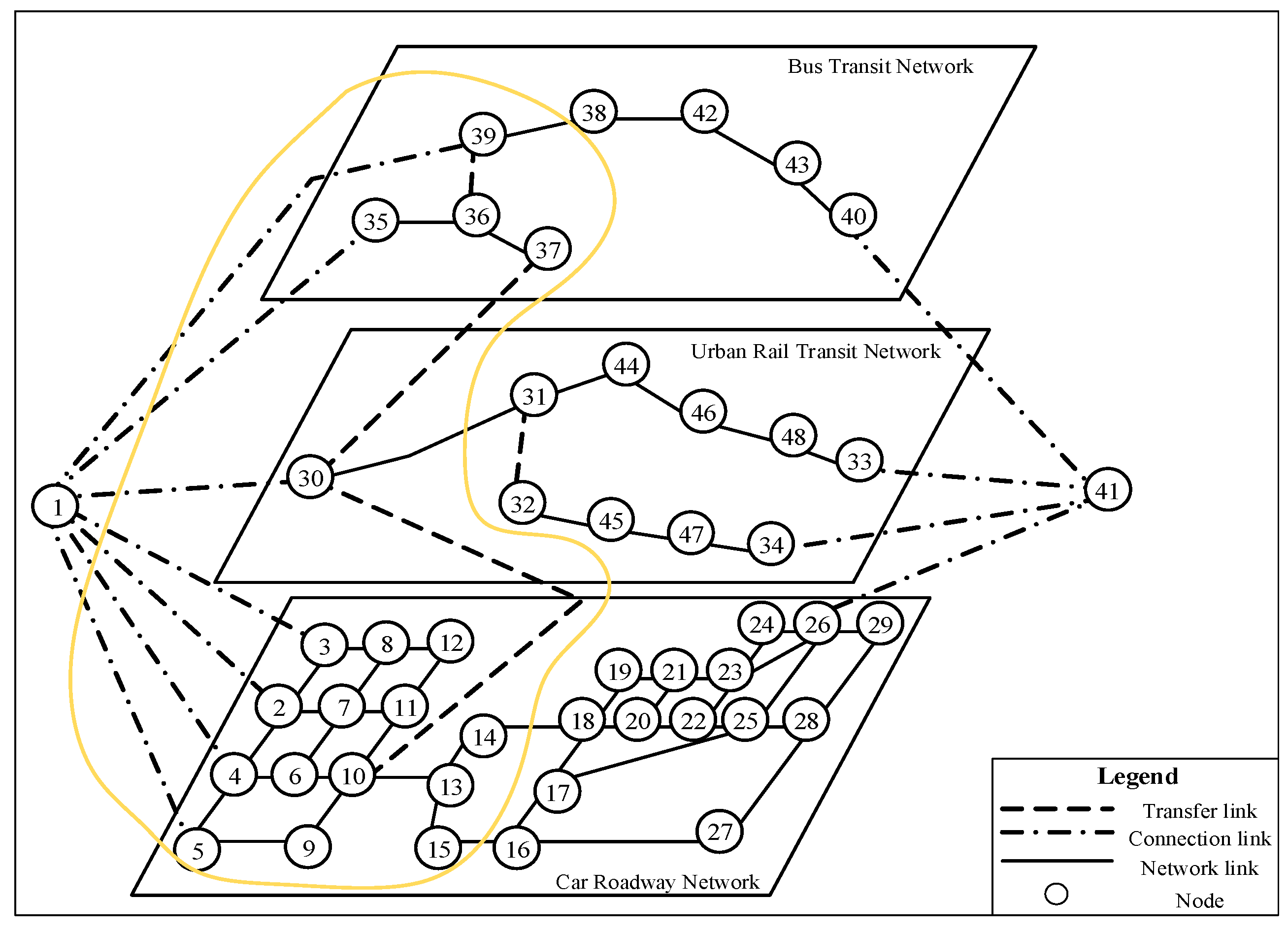
2.2. Topology of Urban Multimodal Transport Network

The term “network” is commonly used to describe a structure that can be either physical or conceptual. Each of these networks includes two types of elements: a set of points and a set of line segments connecting these points. This observation leads to the mathematical definition of a network as a set of nodes and a set of links connecting these nodes [13].

In this paper, the urban multimodal transport network consisted of roadway network, transit networks (bus sub-transport network, urban rail transit sub-transport network), and a connection network, in which we considered five typical transport modes (car, bus, metro, bus-to-metro, and car-to-metro).

In the case of the roadway network, there is only one link between two nodes, in which intersections are regarded as nodes. Similarly, transit nodes are composed of a different set of characteristics than highway nodes. The nodes are called stops, and the lines are called links or route segments. Links in a multimodal transit network have different characteristics from those in a road network. While a link in a road network is a physical segment that connects one node to another, a link in a multimodal transit network is part of the transit line that serves a sequence of transit stops (nodes).

Transfer hubs are groups of nodes that are defined by the ease of transfer between transit lines or modes. Corresponding to the typical combined transport modes, bus-to-metro and car-to-metro, this research defined two types of transfer hubs (bus–metro transfer hub and park and ride (P + R) hub) as nodes in the transfer process, and the group of links among transfer hubs were regarded as the transfer virtual links. Figure 1 displays the schematic topology of the urban multimodal transport network.

2.3. Impedance Function of Links and Paths

Each network link is typically associated with some impedance that affects the flow using it. Impedance can represent time, cost, utility, or any other relevant measure. The units of measurement of this impedance depend on the nature of the network and the link flows. Only links can be associated with impedance. Nodes represent merely the intersection of links and are not associated with any impedance to flow. Travelers choose the transport mode with the least generalized travel cost, which consists of time, cost, and comfort loss in this paper, which is expressed as shown in Equation (1).

$$I_a=T_a+P_a+D_a,$$

(1)

where $I_a$ is the impedance function of link $a$, $T_a$ is the time cost of link $a$, $P_a$ is the fare cost of link $a$, and $D_a$ is the comfort loss of link $a$.

The connection network in this paper refers to the access segment from the origin to the network and the egress segment from the network to the destination by walking. Thus, the components of connection network impedance can be expressed as shown in Equation (2).

$$\begin{array}{c}{T}_a^u=t_a^{u0}+t_a^{u1}, a\in A^u,\\ P_a^u=\eta \times \cos t^u,\\ D_a^u=0, \end{array}$$

(2)

where $T_a^u$ is the impedance function of link $a$ in the access connection network, $t_a^{u0}$ is the walk time cost of link $a$ in the access connection network, $t_a^{u1}$ is the mean waiting time cost of link $a$ in the access connection network, $A^u$ is the set of access links, $P_a^u$ is the fare cost of link $a$ in access connection network, if the transport mode chosen is car,$P_a^u=0$, $\eta$ is the fare cost–time dimension conversion parameter, $\cos t^u$ is the fare cost of bus or metro, and $D_a^u$ is the comfort loss of link $a$ in access connection network.

Similarly, the impedance of egress segment in connection network only involves walking time, as expressed in Equation (3).

$$\begin{array}{c}{T}_a^d=t_a^{d0}, a\in A^d,\\ P_a^d=0,\\ D_a^d=0,\end{array}$$

(3)

where $t_a^{d0}$ is the walk time cost of link $a$ on egress connection network, and $A^d$ is the set of egress links.

The main factors associated with multimodal transport are variables related to the trip itself, type of origin and destination area, trip type, and trip length. In order to account for the contribution of different transport modes, the travel type in this paper was concentrated on commuting trips. Specially, the characteristics of three unimodal transport modes are the road capacity, road length, fuel charge, bus/metro ticket fee, bus/metro capacity, designed passenger volume of bus/metro, and speed of modes.

The travel time of cars in roadway network is limited by the traffic flow and the road capacity. In this paper, regardless of the intersection delay, the travel time of cars in roadway network was given by the BPR function, as shown in Equation (4).

$$T_a^c=t_a^{c0}\left[1+\alpha {\left(\frac{{\nu }_a}{{\lambda }^c{C}_a^c}\right)}^{\beta }\right], a\in A^c,$$

(4)

where $T_a^c$ is the time cost of link $a$ in roadway network, $t_a^{c0}$ is the free travel time,${\nu }_a$ is the passenger flow on link $a$, ${\lambda }^c$ is the conversion parameter which converts vehicle flow into equivalent passenger flow,$\alpha , \beta$ are the undetermined coefficients, $C_a^c$ is the road capacity of link $a$ in roadway network, and $A^c$ is the set of links in roadway network.

Fuel charge is the main fare cost of car travel on the roadway network. Therefore, the fare cost of cars on the roadway network was calculated as shown in Equation (5).

$$P_a^c=\eta \times \rho \times x_a,$$

(5)

where $x_a$ is the length of link $a$ in the roadway network, and $\rho$ is the fuel fee.

The comfort loss of cars in the roadway network is related to its travel time on road links, which can be expressed as shown in Equation (6).

$$D_a^c=\omega \times S_a^c\times T_a^c,$$

(6)

where $S_a^c$ is the comfort loss per unit time of link $a$ in roadway network, $\omega$ is the comfort loss–time dimension conversion parameter.

This study assumed that buses run in exclusive lanes and, thus, will be less affected by other vehicles. The driving time was taken as relatively fixed. In addition, conventional buses adopt fixed pricing, whose fare is charged while boarding and, thus, cannot be allocated to each link. As the transit fare (bus and metro) was added to the previous access connection network, the fare cost in transit networks (bus and metro) was 0. The comfort loss for bus travelers is not only affected by travel time, but also related to the congested degree in bus vehicles. Overall, the components of link impedance in the bus transit network can be expressed as shown in Equation (7).

$$\begin{array}{c}{T}_a^b=t_a^{b0}, a\in A^b,\\ P_a^b=0,\\ D_a^b=\omega \times S_a^b\times T_a^b+\frac{v_a}{B{C}_a^b}, \end{array}$$

(7)

where $T_a^b$ is the time cost of link $a$ in the bus transit network, $t_a^{b0}$ is the actual driving time of the bus on link $a$, $A^b$ is the set of links in the bus transit network, $S_a^b$ is the comfort loss per unit time of link $a$ in the bus transit network, $B$ is the designed passenger volume of the bus, and $C_a^b$ is the bus capacity of link $a$ in bus transit network.

Similarly, the components of the link impedance in the urban rail transit network can be expressed as shown in Equation (8).

$$\begin{array}{c}{T}_a^m=t_a^{m0}, a\in A^m,\\ P_a^m=0,\\ D_a^m=\omega \times S_a^m\times T_a^m+\frac{v_a}{E{C}_a^m},\end{array}$$

(8)

where $T_a^m$ is the time cost of link $a$ in the urban rail transit network, $t_a^{m0}$ is the actual driving time of the metro on link $a$, $A^m$ is the set of links in the urban rail transit network, $S_a^m$ is the comfort loss per unit time of link $a$ in the urban rail transit network, $E$ is the designed passenger volume of the metro, and $C_a^m$ is the metro capacity of link $a$ in urban rail transit network.

This study considered two types of transfer: internal transfer between transit lines and transfer between different modes. There were also three items composing the impedance of virtual internal transfer links, as expressed in Equation (9).

$$\begin{array}{c}{T}_a^i=t_a^{i0}+t_a^{i1}, a\in A^i,\\ P_a^i=\eta \times \cos t^i,\\ S_a^i=penalt{y}_a^i,\end{array}$$

(9)

where $T_a^i$ is the time cost of link $a$ in the virtual internal transfer network, $t_a^{i0}$ is the walk time of link $a$ in the virtual internal transfer network, $t_a^{i1}$ is the mean waiting time of link $a$ in the virtual internal transfer network, $A^i$ is the set of links in the virtual internal transfer network, $P_a^i$ is the fare cost of link $a$ in the virtual internal transfer network, $\cos t^i$ is the transit fare of transferring between bus lines or metro lines, $S_a^i$ is the transfer penalty of link $a$ in the virtual internal transfer network, and $penalt{y}_a^i$ is the convert transfer penalty into equivalent in-vehicle time.

Bus-to-metro and car-to-metro are the two typical combined modes in an urban multimodal transport network. The corresponding transfer hubs considered in this paper were bus–metro transfer hubs and P + R transfer hubs, and the impedance formulas of the transfer hub virtual links were expressed as shown in Equations (10) and (11).

$$I_a^g=t_a^{g0}+t_a^{g1}+\eta \times \cos t^g+penalt{y}_a^g, a\in A^g,$$

(10)

$$I_a^d=t_a^{d0}+t_a^{d1}+\eta \times \left(\cos t^d+par{k}^d\right), a\in A^d,$$

(11)

where $I_a^g$ is the impedance function of link $a$ in the virtual bus–metro transfer network, $I_a^d$ is the impedance function of link $a$ in the virtual P + R transfer network, $t_a^{g0}$ is the walk time of link $a$ in the virtual bus–metro transfer network, $t_a^{g1}$ is the mean waiting time of link $a$ in the virtual bus–metro transfer network, $\cos t^g$ is the transit fare of transferring from bus to metro, $A^g$ is the set of links in the virtual bus–metro transfer network, $t_a^{d0}$ is the walk time of link $a$ in the virtual P + R transfer network, $t_a^{d1}$ is the mean waiting time of link $a$ in the virtual P + R transfer network, $\cos t^d$ is the transit fare of transferring from car to metro, $par{k}^d$ is the parking fare of the car, and $A^d$ is the set of links in the virtual P + R transfer network.

The impedance along a path is the sum of the impedances along the links comprising that path. As for the five transport modes in urban multimodal transport network mentioned before, the expressions of path impedance function for three types of single modes were as follows:

$$\begin{array}{ll}{I}_a^{car}=t_a^{u0}+t_a^{u1}& +\eta \\ & \times \cos t^u+t_a^{d0}+t_a^{c0}\left[1+\alpha {\left(\frac{{\nu }_a}{{\lambda }^c{C}_a^c}\right)}^{\beta }\right]+\eta \times \rho \times x_a+\omega \times S_a^c\times T_a^c, a\\ & \in A^c. \end{array}$$

(12)

$$\begin{array}{ll}{I}_a^{bus}=t_a^{u0}+t_a^{u1}& +\eta \times \cos t^u+t_a^{d0}+t_a^{b0}+\omega \times S_a^b\times T_a^b+\frac{v_a}{B{C}_a^b}+t_a^{i0}+t_a^{i1}+\eta \times \cos t^i\\ & +penalt{y}_a^i, a\in A^b. \end{array}$$

(13)

$$\begin{array}{cc}{I}_a^{metro}=t_a^{u0}+t_a^{u1}& +\eta \times \cos t^u+t_a^{d0}+t_a^{m0}+\omega \times S_a^m\times T_a^m+\frac{v_a}{E{C}_a^m}+t_a^{i0}+t_a^{i1}\\ & +\eta \times \cos t^i+penalt{y}_a^i, a\in A^m.\end{array}$$

(14)

According to the link impedance function of each sub-transport network and virtual link impedance function of transfer hubs introduced above, the two types of combined modes were as follows:

$$I_a^{bus-metro}=T_{a1}^u+P_{a1}^u+T_{a2}^b+D_{a2}^b+I_{a3}^d+T_{a4}^m+D_{a4}^m+T_{a5}^d, a1,\dots ,a5\in a,$$

(15)

$$\begin{array}{cc}{I}_a^{car-metro}=T_{a6}^u& +P_{a6}^u+T_{a7}^c+P_{a7}^c+D_{a7}^c+I_{a8}^g+T_{a9}^m+D_{a9}^m +T_{a10}^d, a6,\dots ,a10\\ \in a,\end{array}$$

(16)

where $a1$ is the link of the access connection network, $a2$ is the link of the bus transit network,$a3$ is the link of the virtual bus–metro transfer network,$a4$ is the link of the urban rail transit network,$a5$ is the link of the egress connection network, $a6$ is the link of the access connection network, $a7$ is the link of the roadway network, $a8$ is the link of the virtual P + R transfer network, $a9$ is the link of the urban rail transit network, and $a10$ is the link of the egress connection network.

2.4. Model Formulation and Solution Algorithm

SUE is the most widely used network flow model, which is suitable for describing a user’s probabilistic route choice in a congested multimodal network [14]. The objective function is to minimize the generalized cost of travelers, and the flow follows the principle of user equilibrium. The assignment assumes that travelers choose the path with the smallest cost. However, travelers will consider transferring to other network to achieve the whole equilibrium of a multimodal transport network when the users and cost of a network increase. Given the OD pair set $W$, the SUE model used in the evaluation process was required to have the following characteristics:

$$\begin{array}{lll}\min Z& (f)=& \frac{1}{\theta }{\displaystyle \sum _w{\displaystyle \sum _k{f}_k^w\ln f_k^w+{\displaystyle \sum _a{\displaystyle {\int }_0^{x_a}{I}_a(w)dw}}}},\\ & s.t. & {\displaystyle \sum _k{f}_k^w}=q^w,\forall k\in K^w,w\in W\\ & & f_k^w\ge 0,\forall k\in K^w,w\in W\\ & & x_a={\displaystyle \sum _w{\displaystyle \sum _k{f}_k^w}}{\delta }_{a,k}^w,\forall a\in A\end{array}$$

(17)

where $f_k^w$ is the passenger flow on path $k$ between OD pair $w$, $q^w$ is the total passenger flow between OD pair $w$,$\theta =0$ if users do not have any information on the travel cost in a network and they are obliged to choose routes randomly, the perfect information of a network may be given to users if $\theta =\infty$; ${\delta }_{ak}^w$ is the incidence relationship between link and path; if link $a$ is on path $k$ between OD pair $w$, ${\delta }_{ak}^w=1$ and 0 otherwise; $I_a\left(w\right)$ is the flow and cost function of link $a$, and $K^w$ is the set of links.

A solution algorithm based on the Method of Successive Weighted Averages (MSWA) is proposed for solving the SUE passenger distribution problem in a multimodal transport network, which allocates more weights to the later iterations instead of the equal average in the Method of Successive Averages (MSA) [15]. The detailed steps for the solution algorithm are presented below.

• Step 1. Set the number of iterations $n=0$, and the link flow matrix of the urban multimodal transport network $x^{\left(0\right)}=0$.
• Step 2. Calculate the fares of each link $I_a^n$, and obtain path flow and the path fares using Depth First Search (DFS) method. Then, get the shortest path and fares $I_{f,min}$ [16].
• Step3. Get the path flow using the Logit model, yielding auxiliary link flow $y^{\left(0\right)}$.
• Step4. Calculate new link flow matrix using an MSWA scheme, with $d=1$.

  $$x^{n+1}=x^n+{\chi }^n(y^n-x^n).$$

  (18)

  $${\chi }^n=\frac{n^d}{1^d+2^d+\dots +n^d}.$$

  (19)
• Step 5. For an acceptable convergence level $\epsilon$, if $\sqrt{\Sigma {\left(x^{n+1}-x^n\right)}^2}\times {\left(\Sigma x^n\right)}^{-1}\le \epsilon$, stop; otherwise, set $n=n+1$, and go to Step 2.

3. Evaluation Functions

The evaluation function and indicators selected in this paper were considered from three perspectives:

• From the perspective of supply–demand balance level of the overall network, it should be possible to evaluate whether the capacity and service level of network under different OD demand scenarios is on a reasonable scale.
• From the perspective of traffic flow assigned in different networks, it should be possible to evaluate the equilibrium of transport network distribution.
• From the perspective of the percentage of public transit travel, it should be possible to evaluate the proportion of passengers that public transit undertakes, since the public transportation can better balance the passenger flow distribution.

3.1. LOS of Multimodal Transport Nerwork

The quality of service describes how well a transportation facility operates. LOS is a quantitative stratification of a performance measure or measures that represents quality of service, which can be assessed in several ways. The resulting volume-to-capacity (v/c) ratio is defined as the indicator, and the supply–demand balance level of the overall multimodal transport network is comprehensively evaluated according to the weighted average v/c ratio of all links on multimodal transport network, ranging from A to D, where A represents the best and D represents the worst level. The LOS of multimodal transport network can be expressed as shown in Equation (20).

$$LO{S}_j=\frac{{\displaystyle \sum (V_i/C_i\times L_i)}}{{\displaystyle \sum L_i}},$$

(20)

where $LO{S}_j$ is the level of service of multimodal transport, $V_i$ is the passenger flow on link $i$, $L_i$ is the length of link $i$, and $C_i$ is the capacity of link $i$.

As for the multimodal transport network in this paper, intersections and bus or metro stations were regarded as the physical nodes, and the links on the automobile roadway network were the road sections between intersections, while the links on the urban rail transit network and bus roadway network were the transit lines between stations.

Transit capacity is different from highway capacity; it deals with the movement of both people and vehicles, it depends on the size of transit vehicles and how often they operate, and it reflects the interaction of passenger traffic and vehicle flow. Thus, $V_i$ represents the actual passenger flow, and $C_i$ represents the carrying capacity of transit vehicles or the roadway passenger carrying capacity converted from vehicle flow.

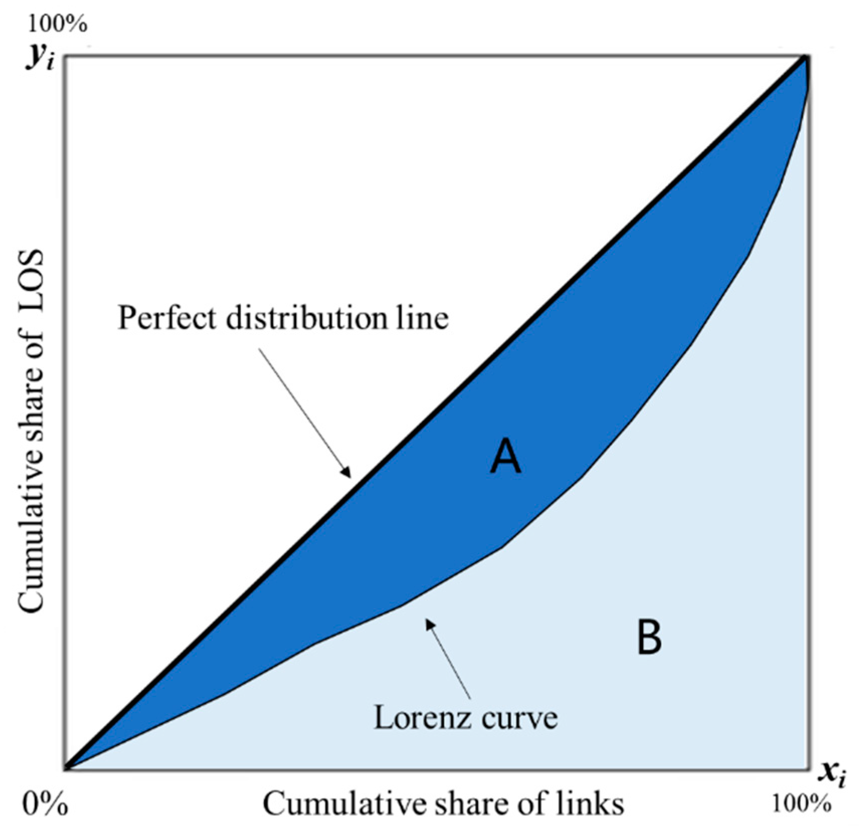
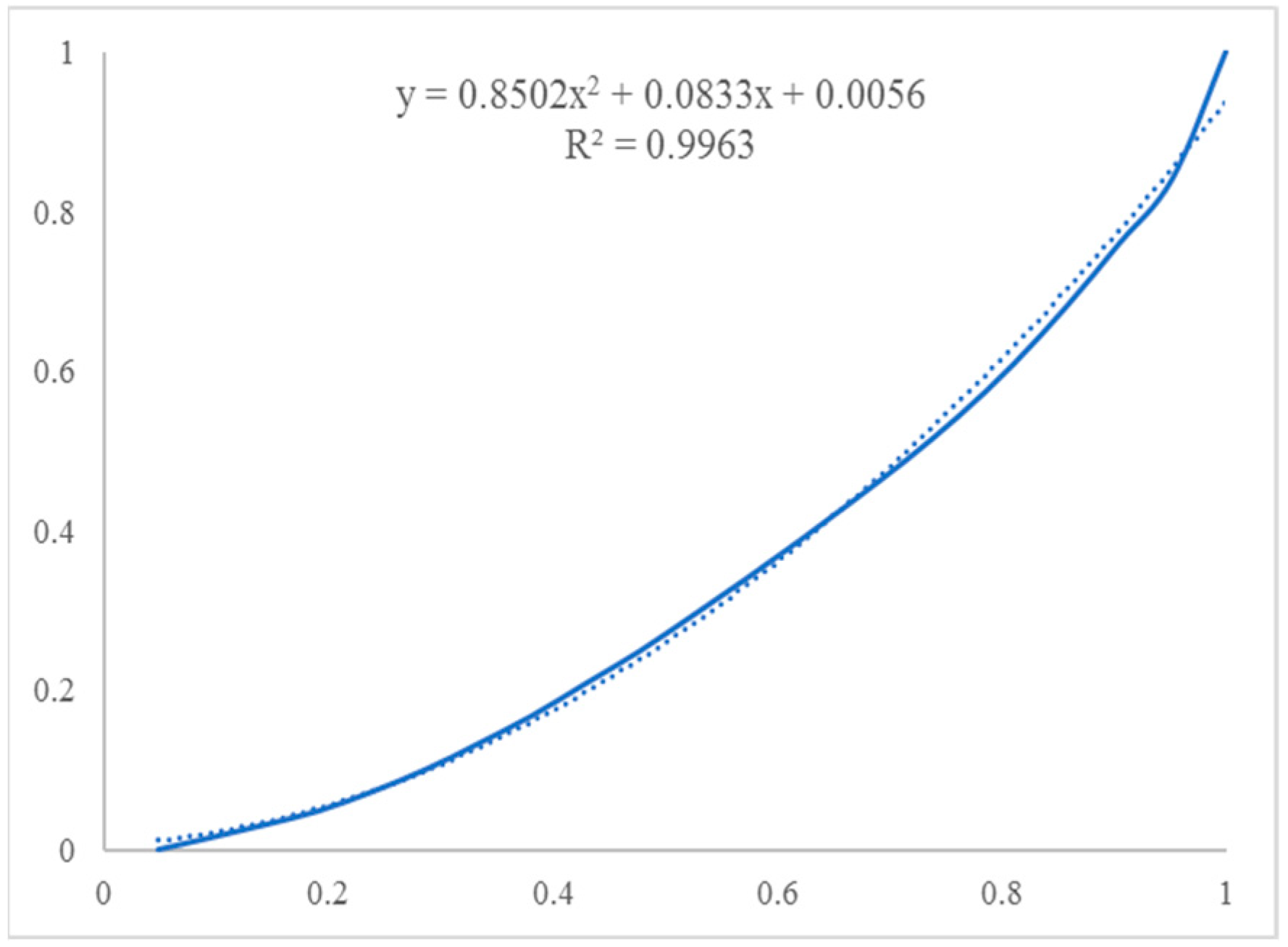
3.2. Gini Coefficient of Multimodal Transport Network

The Gini coefficient was introduced in 1912 as a measure of the inequality of the income distribution in some nation or other society [17]. Its value ranges from 0 to 1. The coefficient approaches 0 as all income differences vanish. It approaches 1 when one person earns all the money, leaving nothing to the remaining inhabitants.

Travel demand in an urban transport network is continuously increasing, and many components of a multimodal transport network are highly congested. The Gini coefficient has long and widely been used in various fields. Specifically, we propose the Gini coefficient, which measures how evenly the passenger flows are distributed across different sub-networks, to provide a key mathematical criterion for evaluating the disparity in service level. The Gini coefficient of a multimodal transport network indicates that a larger value denotes a greater degree of distribution imbalance. This will also help policymakers to deal with the complexity of urban mobility and undertake more sustainable transport network planning.

For the urban multimodal transport network, we denote two cumulative frequencies as $x_i$ and $y_i$, respectively. Clearly, $0\le y_i\le x_i\le 1$. The two proportions can be linked by calculating both $x_i$ and $y_i$ for several different LOS values. Plotting $y_i$ as the ordinate against $x_i$ for all these points and connecting these points results in the Lorenz curve (see Figure 2), which plays an important role in the equilibrium of passenger distribution on different links.

The Lorenz curve is the diagonal of the graph in the case of perfect equality. The Gini index is the fraction of the area between the actual Lorenz curve and the one belonging to perfect equality (see the shaded area A in Figure 2) and the area between the two extrema (that is, A + B). Mathematically, the Gini index is G = A/(A + B); hence, the resulting Gini index is 0 under perfect equality and 1 in the case of perfect inequality.

$$x_i={\displaystyle \sum _j^i\frac{n_j}{N}},$$

(21)

$$y_i={\displaystyle \sum _j^i\frac{LO{S}_j}{{\displaystyle \sum _j^{i}LO{S}_j}}},$$

(22)

where $x_i$ is the cumulative share of numbers of links whose LOS is equal to $LO{S}_j$, $n_j$ is the number of links whose LOS is equal to $LO{S}_j$, $N$ is the number of links on the multimodal transport network, and $y_i$ is the cumulative share of numbers of links whose LOS is equal to $LO{S}_j$.

The Gini coefficient of the multimodal transport network is described by the following equation:

$$G_{in{i}_{LOS}}=A/\left(A+B\right)=1-2{{\displaystyle \int }}_0^{1}f\left(x_i\right)d\left(x_i\right),$$

(23)

where $G_{in{i}_{LOS}}$ is the Gini coefficient of the link LOS, $A$ is the graphic area enclosed by the perfect distribution line and Lorenz curve, and $B$ is the graphic area under the Lorenz curve.

3.3. Mode Share of Transport Modes

Public transit has become one of the main measures to alleviate the problem of urban traffic supply and demand imbalance with the advantages of a large capacity. Under the background that the public transit priority development strategy was widely praised, the public transit in the urban multimodal transport network should undertake the main travel demand among transport modes.

According to the passenger proportion that public transit takes up, the coordination of private and public transport modes can be evaluated by the mode share described in Equation (24), with the criterion on a scale of four levels A to D, where A represents the best and D represents the worst level. There were five transport modes in this study. Public transit modes consisted of metro, bus, and bus-to-metro, whereas private transport modes consisted of car and car-to-metro.

$$ModeShare=\frac{V_B+V_M}{V_B+V_M+V_C}\times 100\%,$$

(24)

where $V_B$ is the passenger flow of a conventional bus, $V_M$ is the passenger flow of the metro, and $V_C$ is the passenger flow of a motor vehicle.

Corresponding to the HCM service level grading (level 6) criterion and the Highway service level grading (level 4) criterion in China, the LOS of the multimodal transport network in this paper was divided into four levels from A to D. Meanwhile, the Gini coefficient criterion of the United Nations regards below 0.2 as perfect equality, between 0.2 and 0.3 as relative equality, 0.3–0.4 as relatively reasonable, 0.4–0.5 as inequality, and more than 0.5 as perfect inequality. As for China’s relevant policies in terms of public transport priority, it is proposed that the mode share of public transport should reach more than 40% in the Chinese megalopolis, that of large cities should reach more than 30%, and that of small and mid-sized cities should reach more than 20%. Accordingly, the criteria for the three evaluation functions and indicators are shown in

Table 1. Evaluation indicators and criteria.

Evaluation Functions	Indicators	Criteria	Results
LOS of multimodal transport network	$LO{S}_j=\frac{{\displaystyle \sum (V_i/C_i\times L_i)}}{{\displaystyle \sum L_i}}$	LOS ≤ 0.3	A
		0.3 < LOS ≤ 0.6	B
		0.6 < LOS ≤ 0.9	C
		LOS > 0.9	D
Gini coefficient of transport network	$G_{in{i}_{LOS}}=A/\left(A+B\right)=1-2{{\displaystyle \int }}_0^{1}f\left(x_i\right)d\left(x_i\right)$	GiniLOS < 0.2	A
		0.2 ≤ GiniLOS < 0.3	B
		0.3 ≤ GiniLOS < 0.4	C
		0.4 ≤ GiniLOS < 0.5	D
		GiniLOS ≥ 0.5	E
Mode share of transport modes	$ModeRatio=\frac{V_B+V_M}{V_B+V_M+V_C}\times 100\%$	ModeShare ≥ 40%	A
		30% ≤ ModeShare < 40%	B
		20% ≤ ModeShare < 30%	C
		ModeShare < 20%	D

.

4. Numerical Example

To test the feasibility and effectiveness of the proposed method, Nanjing city was selected as a case study. Figure 3 shows the research scope of Nanjing city, which is the main commuter corridor from suburban railway station LIUZHOUDONGLU to the central railway station XINJIEKOU. At present, there are more than 100 road links, more than 20 bus links, more than 20 rail links, and two transfer hubs in this scope. The transport network structure is composed of a roadway network, railway network, and bus transit network. Travelers in this area can choose unimodal transport modes including metro, bus, and car or combined modes including bus-to-metro and car-to-metro. The OD demand in this case was assumed to be 7000 during the morning commuter peak.

Table 2. Transport facilities and links of network.

Network Categories	Attributes	Transport Facilities	Number of Links
Roadway network	Expressway	DAQIAOBEI Road, NEIHUANXI Road, HUJUBEI Road	40 + 11 (connection links)
	Arterial road	JIANGSHAN Road, Nanjing Yangtse River Bridge
	Secondary trunk road and branch road	Surrounding Branch roads of HONGWUBEI Road, LIUZHOUDONGLU Railway Station
Bus transit network	Bus line	Bus Line 532	7 (including internal transfer)
		Bus Line 669
Urban rail transit network	Metro line	Metro Line 1	9 (including internal transfer)
		Metro Line 3
Transfer virtual network	Bus-to-metro transfer hub	LIUZHOUDONGLU Railway Station	1
	Car-to-metro transfer hub	WEINISISHUICHENG Bus Station	1

provides the detailed supply facilities and the number of corresponding links in the area.

According to the topology presented before, the 69 links introduced above including the connection network, roadway network, and transit networks were abstracted into a topology structure, where the transfer hubs were regarded as the virtual links, and the nodes were numbered. The final network topology of the actual urban multimodal transport network in this example is shown in Figure 4.

To calculate the impedance function of the 69 links above, it was necessary to calibrate the relevant parameters of the impedance function presented before. The specific values of parameters were set as described in

Table 3. Values of undetermined parameters.

Parameters	Values	Unit	Parameters	Values	Unit
$C_a^c$	1200 (branch road)	pcu/h	$B{C}_a^b$	1200	passengers/hour
	1350 (arterial road)		$E{C}_a^m$	5000	passengers/hour
	1500 (expressway)		$t_a^{u1}$	3	min
	1800 (Nanjing Yangtse River Bridge)		$t_a^{g0}$	7	min
$\eta$	3.02	--	$t_a^{d0}$	10	min
$\alpha$	1.19	--	$penalt{y}_a^i$	10	min
$\beta$	3.09	--	$par{k}^d$	16
${\lambda }^c$	1.4	--	$S_a^c$	0.1	--
$\rho$	0.66	--	$S_a^b$	0.8	--
$\omega$	0.5	--	$S_a^m$	0.5	--

according to [18] and the actual status.

The OD with a travel demand of 7000 passengers was loaded and assigned to different networks using the SUE model and MSWA algorithm. The distribution results of the links surrounded by the transfer hubs in the local multimodal transport network (the part enclosed by the yellow circle in Figure 4) are presented in

Table 4. Passenger distribution results of local case network.

No	Link	Flow	Network	No	Link	Flow	Network
1	1-2	2568	Connection network	19	7-8	647	Roadway network
2	1-3	744		20	7-11	1246
3	1-4	868		21	7-8	975
4	1-5	714		22	8-12	1096
5	1-35	233		23	9-10	788
6	1-30	1856		24	10-13	4682
7	1-39	17		25	10-11	2342
8	2-3	681	Roadway network	26	11-12	1096
9	2-4	1007		27	13-14	2325
10	2-7	880		28	13-15	2357
11	3-8	1425		29	30-31	2295	Urban rail transit network
12	4-5	543
13	4-6	1802		30	35-36	233	Bus transit network
14	4-5	469		31	36-37	227
15	5-9	788		32	36-38	6
16	6-7	940		33	39-40	23
17	6-10	1764		34	10-30	212	Transfer virtual network
18	6-7	902		35	30-37	227

.

5. Results and Discussion

From the passenger distribution results above, the v/c ratio of each sub-transport network and the number of passengers traveling via different transport modes could be calculated, and then the Lorenz curve of the example as drawn as shown in Figure 5.

Furthermore, according to the evaluation functions and calculation Equations (1)–(3), the results of the three types of evaluation indicators under the OD demand of 7000 passengers in this case network were as shown in

Table 5. Evaluation results of indicators.

LOS of Sub-Transport Networks	Passengers of Transport Modes
0.94 (roadway network) 0.09 (bus transit network) 0.21 (urban rail transit network)	23 (bus) 1856 (metro) 227 (bus-to-metro)	4682 (car) 212 (car-to-metro)
Evaluation Functions	Indicators Calculation	Evaluation Results
LOS of multimodal transport network	$LO{S}_j=\frac{{\displaystyle \sum (V_i/C_i\times L_i)}}{{\displaystyle \sum L_i}}=0.64$	C
Gini coefficient of transport network	$\begin{array}{c}Gin{i}_{LOS}=\frac{A}{A+B}=1-2{\displaystyle {\int }_0^{1}L(LO{S}_i)d}(LO{S}_i)\\ =0.3436\end{array}$	C
Mode share of transport modes	$\begin{array}{c}ModeShare=\frac{V_B+V_M}{V_B+V_M+V_C}\times 100\%\\ =30\%\end{array}$	B

.

To demonstrate the effects of different OD demand on the evaluation results, we adopted the proposed evaluation framework in this study by increasing the OD demand from 3000 to 15,000. The calculation results are listed in

Table 6. Results under different OD demand scenarios.

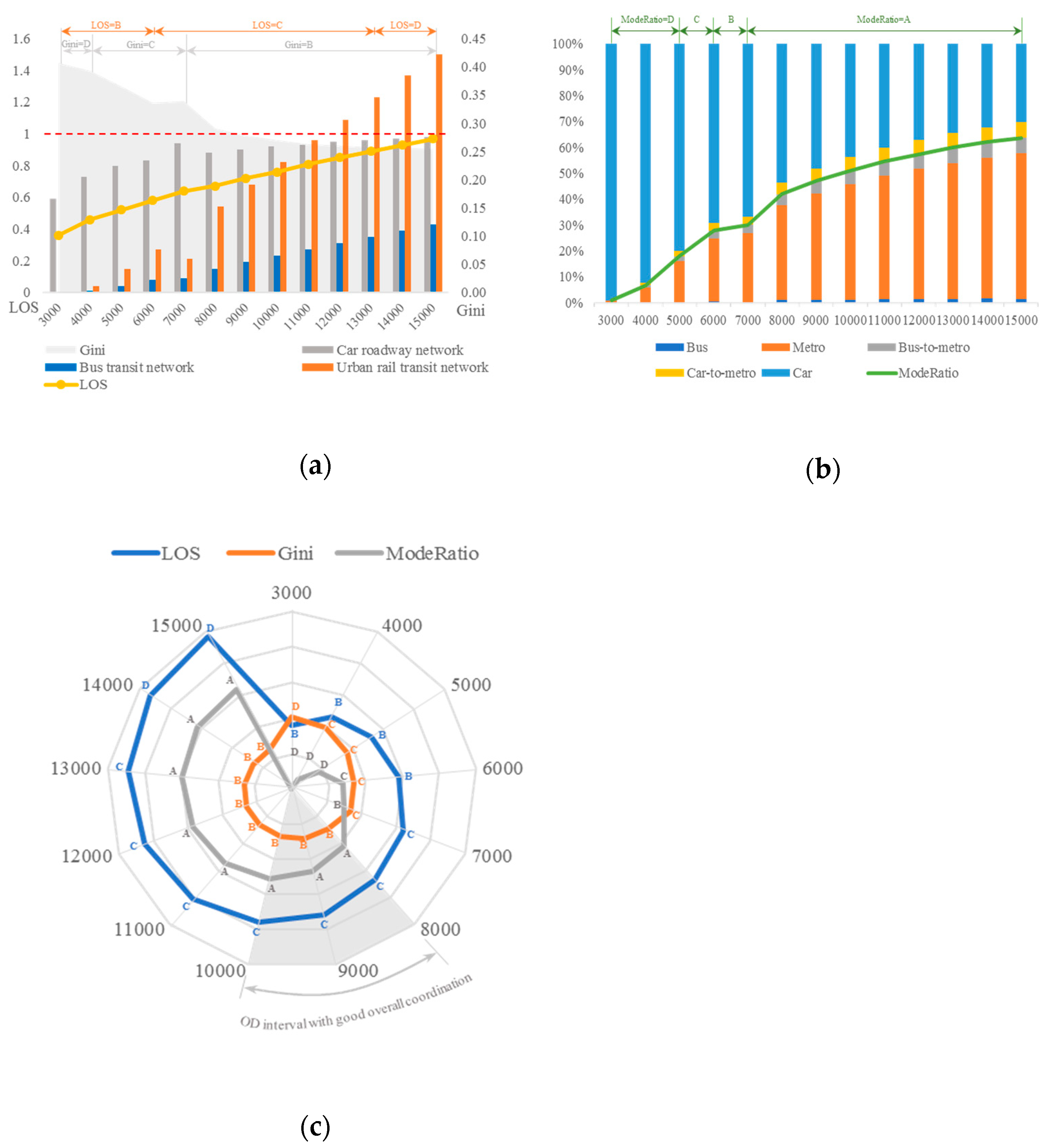
OD Demand	LOS		Gini Coefficient		Mode Share (%)
3000	0.36	B	0.41	D	0.96	D
4000	0.46	B	0.39	C	6.75	D
5000	0.52	B	0.37	C	17.93	D
6000	0.58	B	0.34	C	27.86	C
7000	0.64	C	0.34	C	30.00	B
8000	0.67	C	0.29	B	42.00	A
9000	0.72	C	0.28	B	47.00	A
10,000	0.76	C	0.27	B	51.10	A
11,000	0.81	C	0.26	B	54.50	A
12,000	0.85	C	0.26	B	57.40	A
13,000	0.89	C	0.26	B	59.90	A
14,000	0.93	D	0.26	B	62.00	A
15,000	0.97	D	0.26	B	63.71	A

, and the variation trend of indicators is presented in Figure 6.

As the OD demand was increased from 3000 to 15,000 in Figure 6a, the v/c ratio of each sub-transport network increased, which led to the debasement of service quality of the whole multimodal transport network. For example, with a demand of 3000, the v/c ratio of roadway network was 0.59 while the ratios of other transit networks were small. When the demand increased to 10,000, the v/c ratios of the roadway network and urban rail transit network increased dramatically (from 0.59 to 0.95 and from 0 to 1.09, respectively). This demonstrates that, with the increase in demand, travelers tend to choose a more reliable metro that has no congestion interactions with buses and cars. In view of this, the large OD demand not only results in severe traffic congestion on the road, but also leads to the overload of the rail transit network capacity. When the OD demand reaches 14,000, the LOS of the overall multimodal transport network decreases to the worst level D.

It also can be seen from Figure 6a that the Gini coefficient of the multimodal transport network showed a downward trend with the increase in OD demand. With the demand of 3000, the Gini coefficient was 0.41, close to 0.5, indicating a large imbalance in passenger distribution among different sub-transport networks, and a poor level of coordination and equilibrium. The Gini coefficient decreased with the increase in OD demand and the change in passengers allocated to different networks, indicating a reduction in the distribution gap between different networks and better overall coordination.

In Figure 6b, the percentage modal split for transit modes (bus, metro, bus-to-metro) increased dramatically as the OD demand changed, and the evaluation results of the transit ratio were improved to a good level. For example, the percentage of metro passengers increased from 0.8% to 56.1%. On the contrary, the percentage modal split for cars decreased from 99% to 30.3%. For buses, there was only a slight increase (0% to 1.5%). This may be due to large OD demand resulting in a higher impedance of roadway transport modes than the rail transit mode.

Figure 6c displays the results of the three evaluation functions. As the OD demand changed, the results of evaluating the capacity coordination in the multimodal transport network from three perspectives were different. However, it is difficult to find the optimal situation where all three indicators reached a good level. In this case, a multimodal transport network with good overall coordination under different OD demands was selected when the LOS was no more than 0.8, the Gini coefficient was less than 0.3, and the mode share exceeded 30%. Correspondingly, the OD demand interval was identified as 8000 to 10,000.

6. Conclusions

This research put forward a set of evaluation process for an urban multimodal transport network which considers the roadway network, bus transit network, urban rail transit network, and connection network. For the multimodal network, the paper fully considered the impedance of links in different sub-transport networks and constructed the complete path impedance of five different transport modes (namely, car, bus, metro, bus-to-metro, and car-to-metro). To quantify the passenger distribution in a multimodal transport network, the paper adopted the SUE model to solve the problem, and the results were calculated using the MSWA, which provided the necessary basis for further evaluation.

This research suggested evaluation functions for the indicators from three perspectives. The LOS of the multimodal transport network showed the overall service quality by calculating the v/c ratio of each single network. The Gini coefficient of the network indicated whether most passengers are using a single network, which would result in single-network congestion and disequilibrium of the whole network. The mode share of transport modes reflected the share rate of transit in the multimodal transport network.

The methodology and the evaluation process proposed in the paper were applied to a real example in Nanjing. In this case, some assumptions were adopted. These assumptions may have caused some potential biases. It was assumed that there was only one OD pair with a demand of 7000 commuting passengers during the morning peak. The feasibility of the proposed evaluation process was well proven by the numerical examples using different OD demands. The results of the numerical examples of OD demand ranging from 3000 to 15,000 indicated that, with a small OD demand, the roadway network would take most of the passengers, whereas the distribution among various networks was unbalanced and the transit sharing rate was low. Accordingly, managers can enhance the appeal and reduce the impedance of transit modes by optimizing the facilities of transit networks (i.e., reducing the walking and waiting time). Similarly, the shortcomings of the network can be recognized, which can provide guidance for network optimization and future improvement.

Notably, the current study was limited by data acquisition and the complexity of calculation, and it only focused on assumed OD demand. In practical application, the relevant parameters of the impedance function of each link (e.g., fuel fee and speed) should be accurately calibrated according to the actual situation instead of using fixed constants based on the literature, so that the distribution results become more in line with the actual situation and the assignment results calculated by the model are more accurate.

References

- Driscoll, W.; Larsen, P.B. Convention on International Multimodal Transport of Goods. Tul. L. Rev. 1982, 57, 193. [Google Scholar]
- Lin, J.; Ban, Y. Complex Network Topology of Transportation Systems. Transp. Rev. 2013, 33, 658–685. [Google Scholar] [CrossRef]
- Bevrani, B.; Burdett, R.L.; Yarlagadda, P.K. A case study of the Iranian national railway and its absolute capacity expansion using analytical models. Transport 2017, 32, 398–414. [Google Scholar] [CrossRef] [Green Version]
- Ronald, N.; Arentze, T.; Timmermans, H. Modeling social interactions between individuals for joint activity scheduling. Transp. Res. Part B Methodol. 2012, 46, 276–290. [Google Scholar] [CrossRef]
- Burdett, R. Multi-objective models and techniques for analysing the absolute capacity of railway networks. Eur. J. Oper. Res. 2015, 245, 489–505. [Google Scholar] [CrossRef] [Green Version]
- Burdett, R.; Kozan, E. Techniques for absolute capacity determination in railways. Transp. Res. Part B Methodol. 2006, 40, 616–632. [Google Scholar] [CrossRef] [Green Version]
- Minderhoud, M.M.; Botma, H.; Bovy, P.H.L. Assessment of Roadway Capacity Estimation Methods. Transp. Res. Rec. J. Transp. Res. Board 1997, 1572, 59–67. [Google Scholar] [CrossRef] [Green Version]
- Minderhoud, M.; Tavasszy, L.A.A. Strategic Port Choice Model for Worldwide Container Flows. In Proceedings of the Transportation Research Board 88th Meeting, Washington, DC, USA, 11–15 January 2009. [Google Scholar]
- National Research Council (U.S.). HCM2010: Highway Capacity Manual, 5th ed.; Transportation Research Board: Washington, DC, USA, 2010. [Google Scholar]
- Park, M. Capacity Modeling for Multimodal Freight Transportation Networks; University of California: Irvine, CA, USA, 2005. [Google Scholar]
- Mishra, S.; Welch, T.F.; Jha, M.K. Performance indicators for public transit connectivity in multi-modal transportation networks. Transp. Res. Part A Policy Prac. 2012, 46, 1066–1085. [Google Scholar] [CrossRef]
- Friedrich, M. Evaluating the Service Quality in Multi-modal Transport Networks. Transp. Res. Procedia 2016, 15, 100–112. [Google Scholar] [CrossRef] [Green Version]
- Sheffi, Y. Urban Transportation Networks: Equilibrium Analysis with Mathematical Programming Methods; Yosef Sheffi. Prentice-Hall, Inc.: Englewood Cliffs, NJ, USA, 1984. [Google Scholar]
- Asakura, Y. Evaluation of network reliability using stochastic user equilibrium. J. Adv. Transp. 1999, 33, 147–158. [Google Scholar] [CrossRef]
- Liu, H.X.; He, X.; He, B. Method of Successive Weighted Averages (MSWA) and Self-Regulated Averaging Schemes for Solving Stochastic User Equilibrium Problem. Netw. Spat. Econ. 2009, 9, 485–503. [Google Scholar] [CrossRef]
- Floyd, R.W. Algorithm 97: Shortest path. Commun. ACM 1962, 5, 345. [Google Scholar] [CrossRef]
- Thomas, V.; Wang, Y.; Fan, X. Measuring Education Inequality: Gini Coefficients of Education; Policy Research Working Paper Series 1.100; World Bank Group: Washington, DC, USA, 2001; pp. 43–50. [Google Scholar]
- Meng, M.; Shao, C.; Zeng, J.; Dong, C.; Zhuge, C. Traffic assignment model and algorithm with combined modes in a degradable transportation net-work. J. Cent. South Univ. 2014, 45, 643–649. [Google Scholar]