Abstract
Stress intensity factor (SIF) is one of three important parameters in classical linear elastic fracture mechanics (LEFM). The evaluation of SIFs is of great significance in the field of engineering structural and material damage assessment, such as aerospace engineering and automobile industry, etc. In this paper, the SIFs of a central straight crack plate, a slanted single-edge cracked plate under end shearing, the offset double-edge cracks rectangular plate, a branched crack in an infinite plate and a crucifix crack in a square plate under bi-axial tension are extracted by using the p-version finite element method (P-FEM) and contour integral method (CIM). The above single- and multiple-crack problems were investigated, numerical results were compared and analyzed with results using other numerical methods in the literature such as the numerical manifold method (NMM), improved approach using the finite element method, particular weight function method and exponential matrix method (EMM). The effectiveness and accuracy of the present method are verified.
1. Introduction
In the field of fracture mechanics, the stress field near the crack tip is usually described by the SIFs. For brittle materials, it can also be used to describe the non-singular stresses on the crack surface. The SIF is of great significance for the research of material fracture and crack propagation in practical engineering problems. At present, there have been many numerical methods which were applied to solve the SIFs, such as the traditional finite element method (FEM) and boundary element method (BEM), extended finite element method (XFEM), meshless method (MLM), EMM, the improvement of the FEM, the particular weight function method and NMM, etc. After many efforts of numerous researchers, many methods were also used to extract the SIFs, such as the extrapolation method, interaction integral method and J integral method, etc.
In the past twenty years, the XFEM has mostly been used to analyze fracture mechanics problems. The XFEM is based on the partition of the unity finite element method, adding the step function and the asymptotic field of crack tip displacement to describe the crack, and has achieved fruitful results in the analysis and research of discontinuous problems such as crack and crack propagation [1,2,3,4,5]. The EMM [6] converts the linear, elastic, two-dimensional and steady-state equations of the crack problem into a Hamiltonian system. By changing the angular stress to the radial stress, the eigensolutions satisfying the adjoint symplectic orthogonality are obtained, and then the desired solution of the problem is obtained by using the linear combination of these eigensolutions. The improved finite element method [7] divides the whole crack region into two sub-regions, namely the complementary energy sub-region around the crack tip and the potential energy sub-region of the rest regions, which is an improved method to extract the SIF by using the FEM. The particular weight function method [8] uses the specified reference loading conditions on both sides of the crack for finite element analysis, deduces the coefficients of each weight function, and then computes the SIF under loading by using the weight function.
In the past few decades, the P-FEM and the CIM have been applied to extract the SIFs of the materials and structures, but most of the research is to use separately the P-FEM or using traditional low-order FEM and the CIM or the CIM in combination with other methods such as the displacement discontinuity method [9]. Currently, there are a few works for the P-FEM combined with the CIM to extract SIFs [10,11].
This study aimed to provide a simple, direct, and accurate numerical method to extract the SIFs for the single and multiple crack problems. The effectiveness and performance of this method are verified by numerical examples. In this paper, the commercial finite element software StressCheck developed by the American ESRD (Engineering Software Research and Development) company was used as a simulation tool. Numerical models will demonstrate that the present method is effective not only for the single-crack problems but also for multiple-crack problems in the analysis of fracture mechanic problems. The present method works as follows: firstly, the P-FEM is employed to obtain a highly accurate displacement field and stress field, and then SIFs are derived through the super-convergent CIM. The SIFs for a central straight crack plate, a slanted single-edge crack plate, the offset double-edge cracks in the rectangular plates, a branched crack in an infinite plate and a crucifix crack in a square plate were evaluated using the present method, and compared with the published results using the NMM, improved approach finite element method, particular weight function method and EMM in the literature.
2. P-Version Finite Element Method
2.1. Development of P-FEM
In past three decades, the P-FEM has been developed rapidly and its mathematical theory has been established completely. The convergence of numerical solutions of P-FEM has also been strictly proved, and its error estimation has also been obtained [12,13,14]. Compared with the traditional FEM, the P-FEM has the advantages of less preprocess, faster convergence rate and higher accuracy.
At present, the P-FEM has been widely used in various engineering practice fields, and has obtained fruitful research results. The P-FEM has been applied to the unsteady temperature field problem [15], beam vibration problem [16,17,18] and micro rectangular plate thermal buckling analysis [19]. In the three-dimensional elastic viscoelastic problems in the hydraulic structure [20], seepage analysis [21], the mechanical response of the arteries in the field of biomechanics of bone problems [22] and sandwich and Kirchhoff plate deformation analysis [23,24], the P-FEM has been also successfully applied. The application of P-FEM in elastic fracture mechanics (including the calculation of SIF and predicting the growth of irregular crack fronts) can be found in references [25,26,27,28,29].
2.2. Shape Functions of the P-FEM
For two-dimensional problems, there are usually two types of shape functions (interpolation shape function and hierarchic shape function) defined in standard quadrilateral element and triangular element :
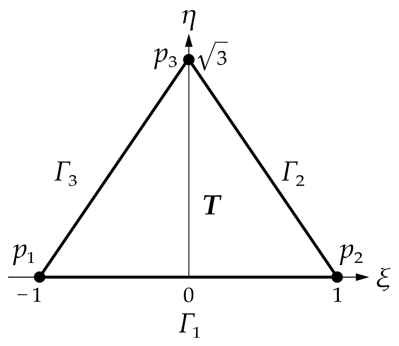
Taking a two-dimensional standard triangle element (as shown in Figure 1) as an example, the high-order hierarchic shape function of the P-FEM on the standard triangle element is constructed as follows [30]:
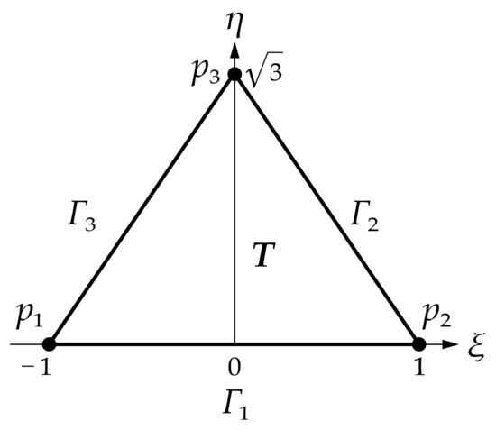
Figure 1.
Standard triangle element .
2.2.1. Nodal Modes Shape Functions for
The nodal modes shape function is the shape function related to nodes. The nodal modes shape function for p = 1 is the same as the conventional Lagrangian interpolation function. Taking the standard triangle element as an example, the nodal modes shape function are as follows:
2.2.2. Side Modes Shape Functions for
The side modes shape functions are the shape functions related to the edges. For example, the side modes shape function of the edge is the shape function related to the corresponding side . The side modes shape function associated with the edge is defined as follows:
where
is Legendre polynomial of :
Similarly, the side modes shape functions associated with the side are defined as:
2.2.3. Internal Modes Shape Functions for
When ,
When , the new internal modes shape function is added:
Similarly, when , the new internal modes shape function is added:
where is the Lagrange interpolation polynomial, and
The number of hierarchic shape functions is determined by the degree p. In this paper, the triangular element and high-order hierarchic shape functions are used to calculate the stresses and strains near the crack tip, and the computation is carried out under the condition of .
3. Contour Integral Method
The CIM is a super-convergent numerical method based on the Betti’s theorem of reciprocal works. In recent years, the CIM has been widely used in various fields to solve various practical or theoretical problems, and has yielded many excellent results. For example, Pereira et al. [31] analyzed the loading crack based on the CIM and the generalized finite element method. Leblanc et al. [32] solved the acoustic nonlinear eigenvalue problem based on the CIM. Garzon et al. [33] studied the three-dimensional crack problems based on the CIM and truncation function method. Feng et al. [34] analyzed the reflection radiation error between turbine blades and blades in computational fluid dynamics based on the CIM. Cui et al. [9] calculated the SIFs based on the CIM and displacement discontinuity method.
In this paper, the CIM proposed by Szabó et al. [35] and Pereira et al. [31] is adopted to extract the SIFs of the single- and multiple-crack problems. The detailed discussions about the CIM were reported in [31,35]. According to Pereira et al. [31], the SIFs can be obtained by calculating the follow integrals:
where and are traction vectors respectively calculated by and , which are the export functions respectively corresponding to modes I and II SIFs, and their definitions are as follows:
The SIFs and calculated by Equations (11) and (12) are exact. Definitions of symbols in Equations (11)–(14) refer to [31]. Due to the reason that displacement field and the corresponding traction vector are unknown, based on the P-FEM, the approximate solution of and the approximate solution of is obtained, and the numerical solutions of the SIFs and are finally extracted. The selection of contour in the computation is flexible and important. Generally, we choose the contour surrounding the innermost elements near the crack tip.
4. Numerical Examples
4.1. A Central Straight Crack Plate
In order to demonstrate the validation of the present approach, the first benchmark example is a central straight crack plate subjected to a uniform uniaxial tension on the upper and bottom edges shown in Figure 2. For this example, the length of the plate is , the width is , the ratio of crack length to width = 0.1, 0.2, 0.3, 0.4, 0.5, 0.6 and 0.7 are considered, and the plane stress condition is assumed. The material parameters are elastic modulus , Poisson’s ratio . The analytical solution of the SIF for this model is given in [36] as follows:
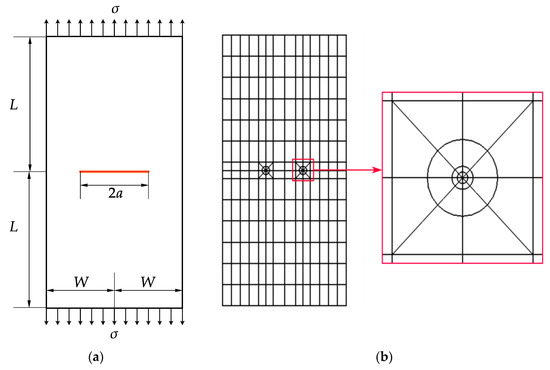
Figure 2.
(a) A central straight crack plate; (b) Global and local meshes (the total number of elements is 252).
For this simulation, 252 elements are used for discretization (as shown in Figure 2b). The computation results of the SIF are summarized in Table 1 and Table 2 for the case a/W = 0.1, 0.2, 0.3, 0.4, 0.5, 0.6 and 0.7. The errors of energy norm of the P-FEM solutions and relative errors of the SIFs for the example are listed in Table 1; here we only list the results for the case , the results for other cases are similar. It can be seen from Table 2, compared with the high-order NMM [37], that an obvious improvement in accuracy is observed.

Table 1.
Errors of energy norm of the P-FEM solutions and relative errors of the SIFs (a/W = 0.4, DOF: degree of freedom).
Table 2.
SIFs for central straight crack plate.
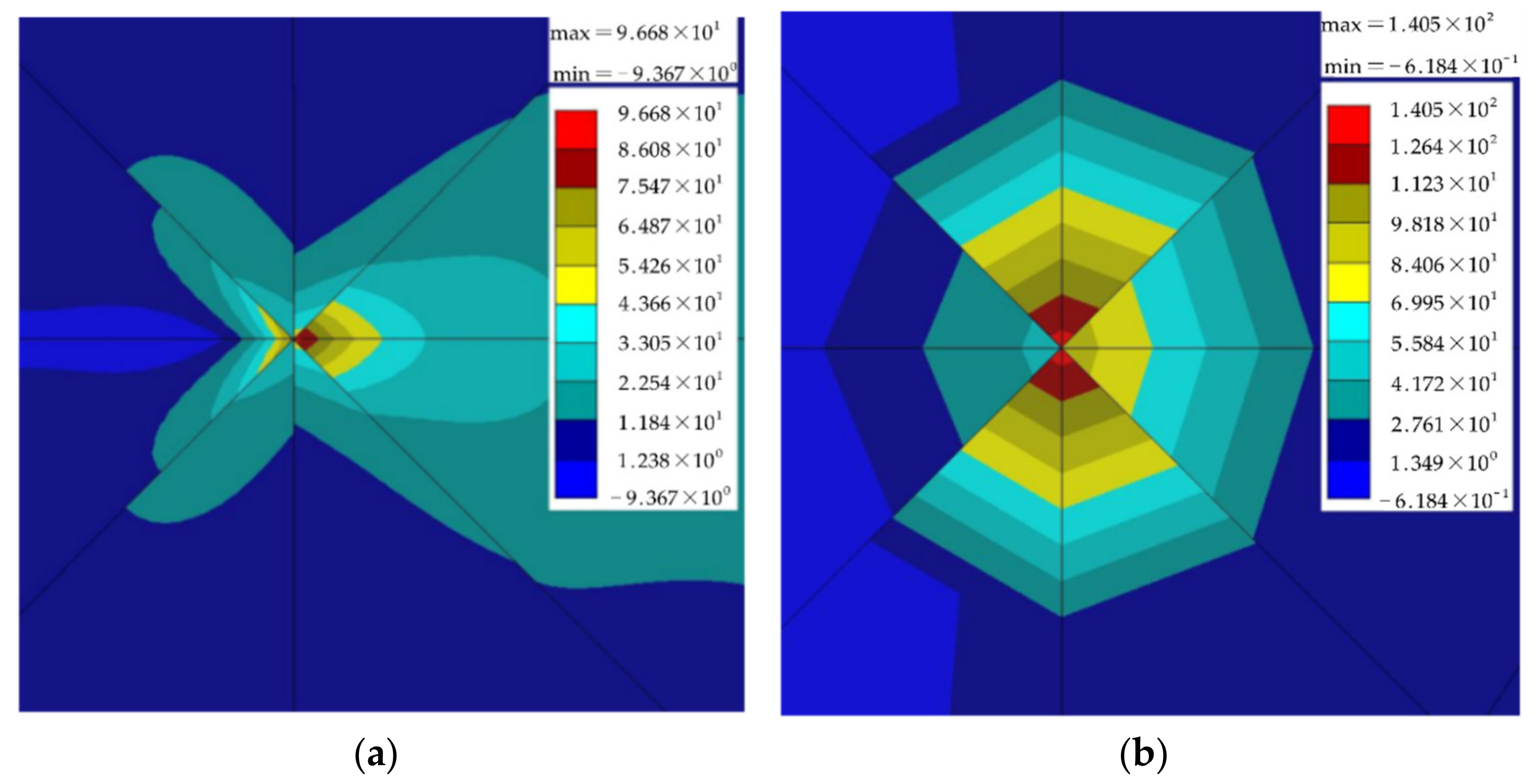
The stress nephogram of the example is shown in Figure 3. For the sake of simplicity, only the stress nephogram for the first example is plotted, the others are similar.

Figure 3.
The stress nephogram at the left crack tip: (a) x-axis direction; (b) y-axis direction.
4.2. A Slanted Single-Edge Crack Plate
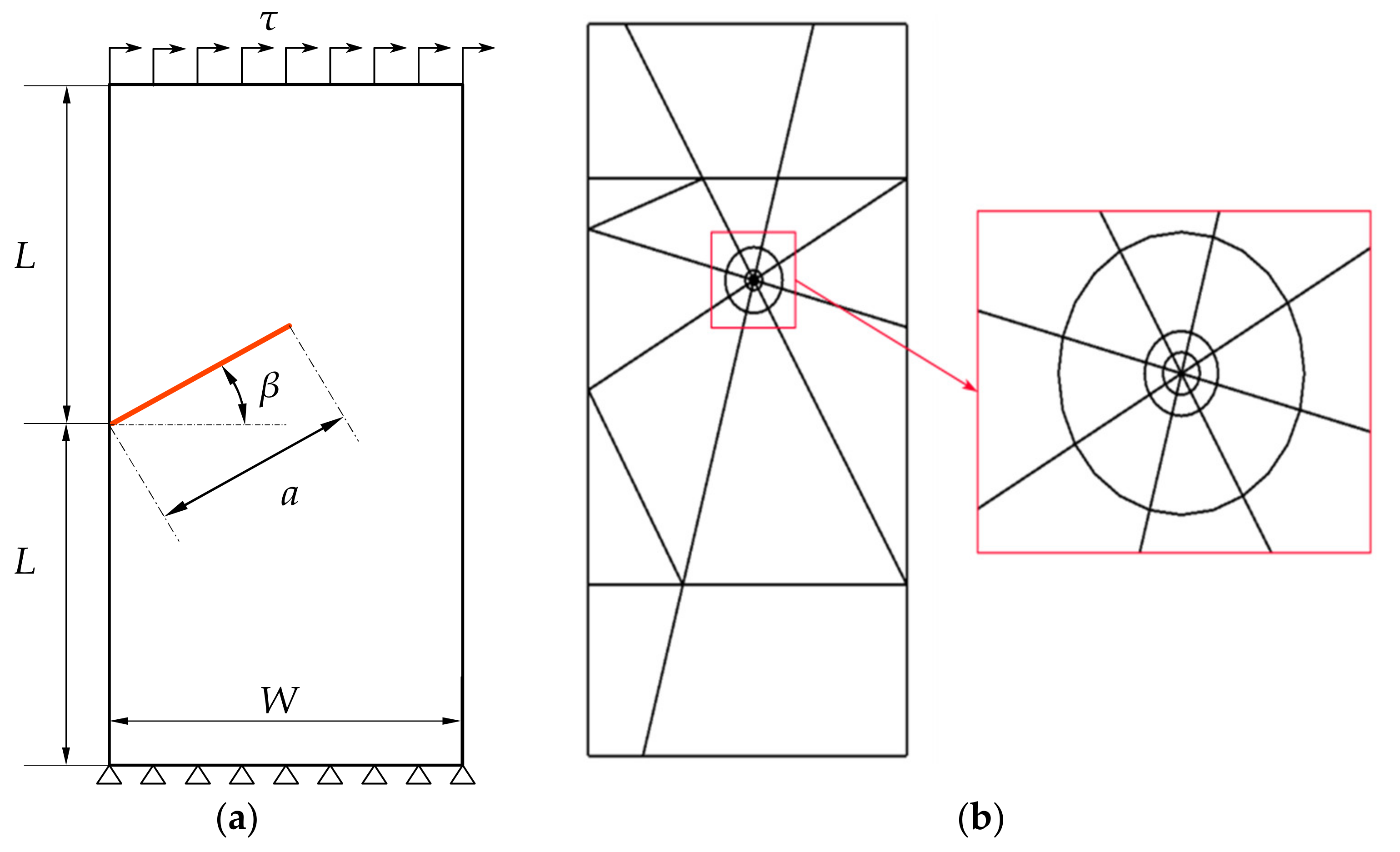
The rectangular plate under end shearing with oblique crack is shown in Figure 4. The bottom of the model is fixed, and the top is imposed to mixed-mode shear load , where , the initial crack length , and the initial crack direction . The material parameters of the model are elastic modulus, , Poisson’s ratio . The model is computed under plane stress condition.
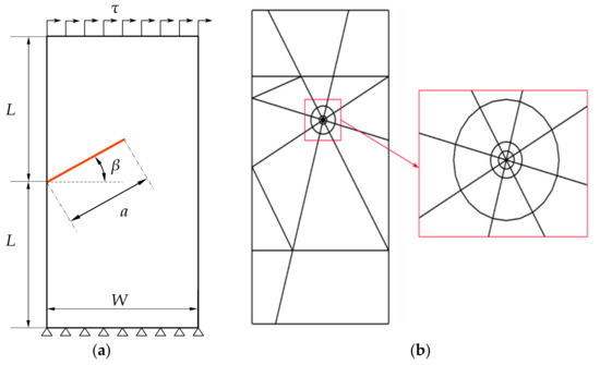
Figure 4.
(a) A slanted single-edge cracked plate under end shearing; (b) Global and local meshes (the total number of elements is 39).
The present computation results are shown in Table 3, compared with results in the literature [6,38], which are in good agreement and verify effectiveness of the present method. The results , , in [6] are referred as the reference solutions, the present computation results are , , . The relative errors of , , and are 0.024%, 0.022% and 0.0138% respectively.
Table 3.
Normalized SIF for a slanted-edge crack plate under end shearing.
The errors of energy norm of the P-FEM solutions and relative errors of normalized SIFs comparison with Abaqus solutions [6] for the example are listed in Table 4.
Table 4.
Errors of energy norm of the P-FEM solutions and relative errors of normalized SIFs comparison with Abaqus solutions [6].
4.3. The Offset Double Edge Cracks Plate
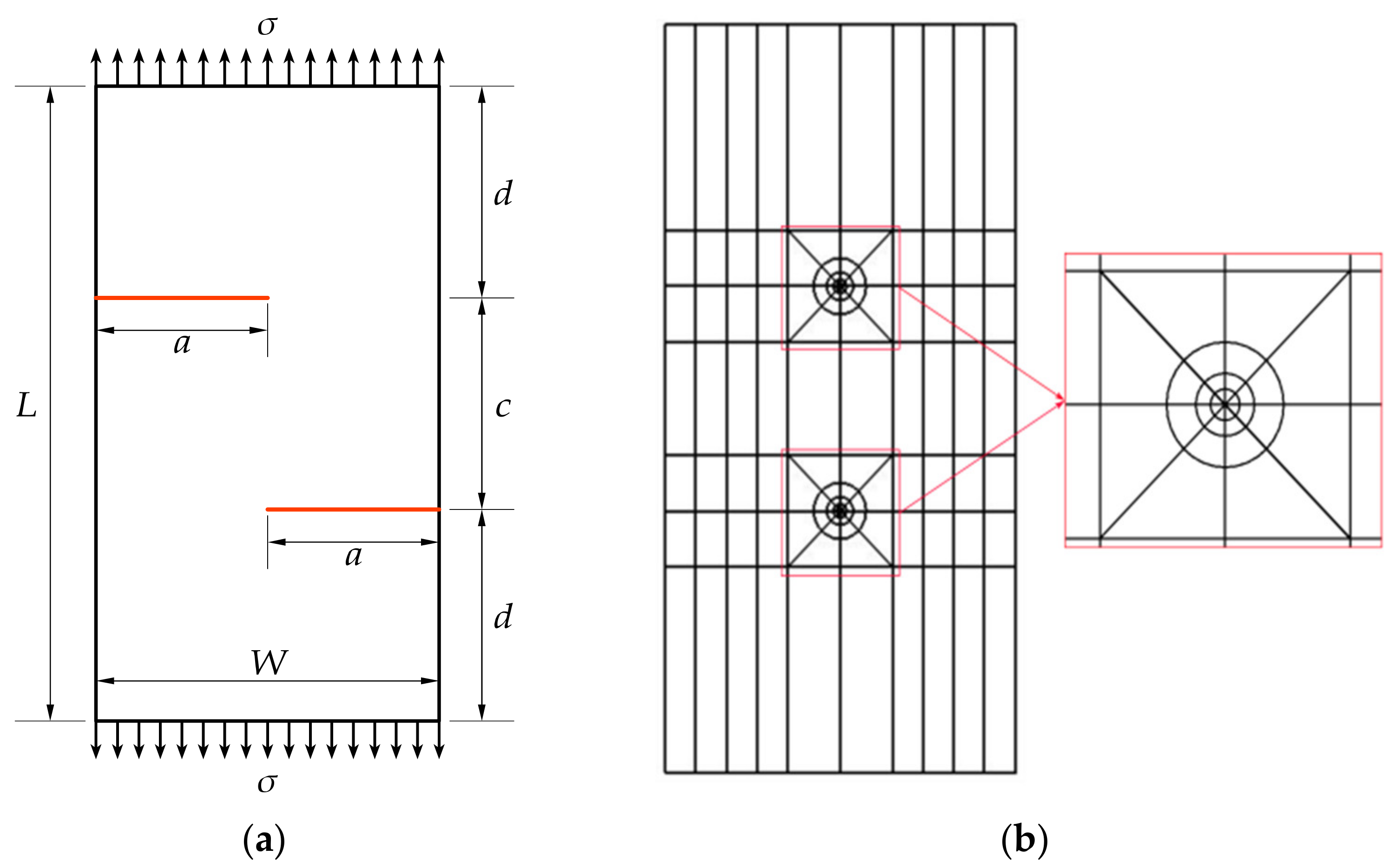
The rectangular plate with the offset double-edge cracks is shown in Figure 5. The top and bottom of the model are subjected to uniformly distributed tensile load , the geometric size of the model is , where , and the initial crack length on both sides is . The material parameters of the model plate are elastic modulus , Poisson’s ratio , and the plane stress condition is assumed.
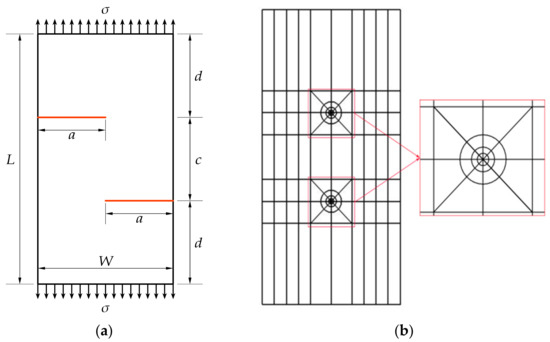
Figure 5.
(a) Rectangular plate with the offset double-edge cracks; (b) Global and local meshes (the total number of elements is 142).
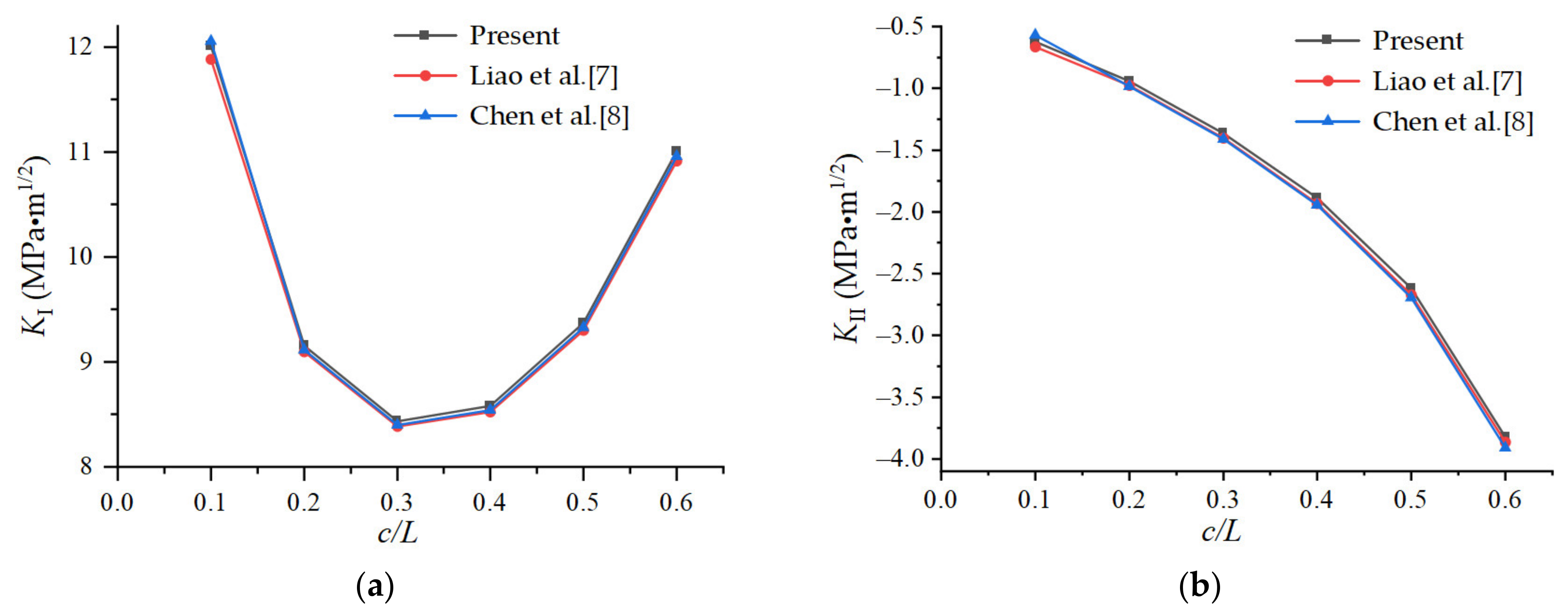
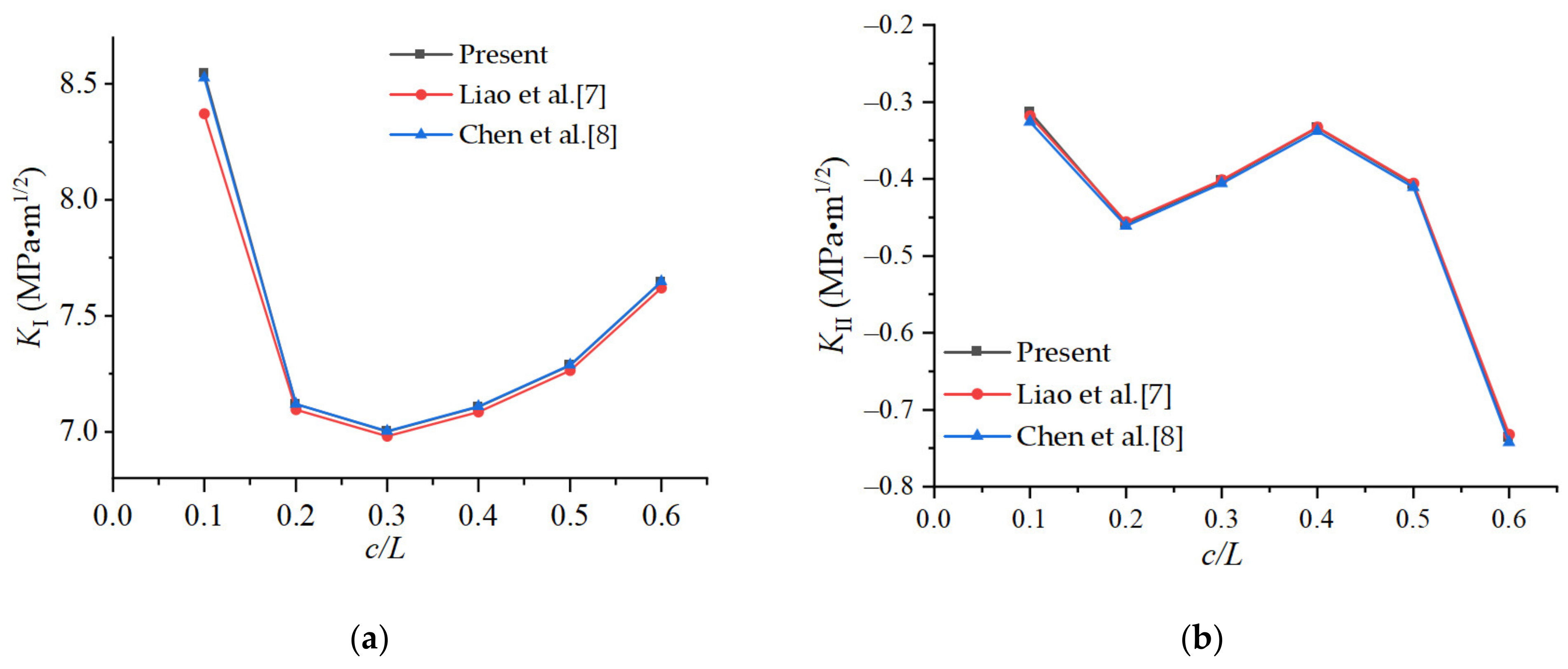
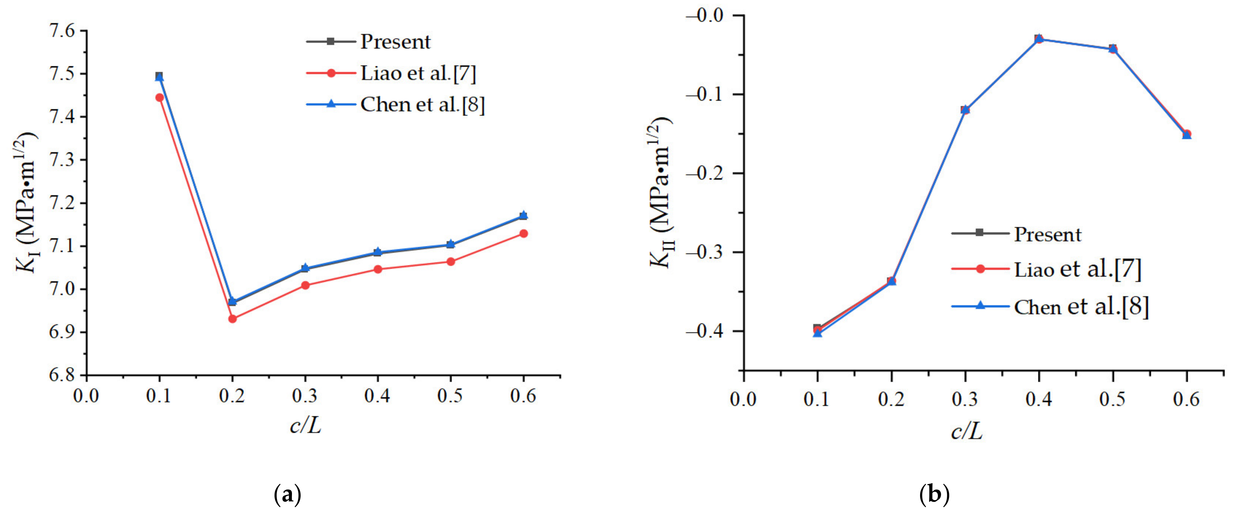
The SIFs under various crack spacing conditions are computed, and the influence of the ratio of length to width of different plates is also considered, as shown in Table 5, Table 6 and Table 7. The present results are in good agreement with those in the literature [7,8], as shown in Figure 6, Figure 7 and Figure 8.
Table 5.
SIFs with different crack spacing (L/W = 1).
Table 6.
SIFs with different crack spacing (L/W = 2).
Table 7.
SIFs with different crack spacing (L/W = 3).
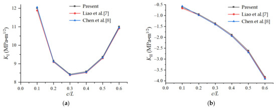
Figure 6.
SIFs for different crack spacings (L/W = 1): (a) SIFs ; (b) SIFs .
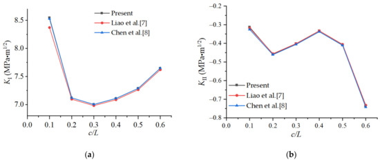
Figure 7.
SIFs for different crack spacing (L/W = 2): (a) SIFs ; (b) SIFs .
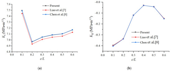
Figure 8.
SIFs for different crack spacing (L/W = 3): (a) SIFs ; (b) SIFs .
The errors of energy norm of the P-FEM solutions and relative errors of SIFs comparison with Chen et al. [8] for the case , are listed in Table 8, the others are similar.
Table 8.
Errors of energy norm of the P-FEM solutions and relative errors of SIFs (L/W = 3, c/L = 0.3) comparison with Chen et al. [8].
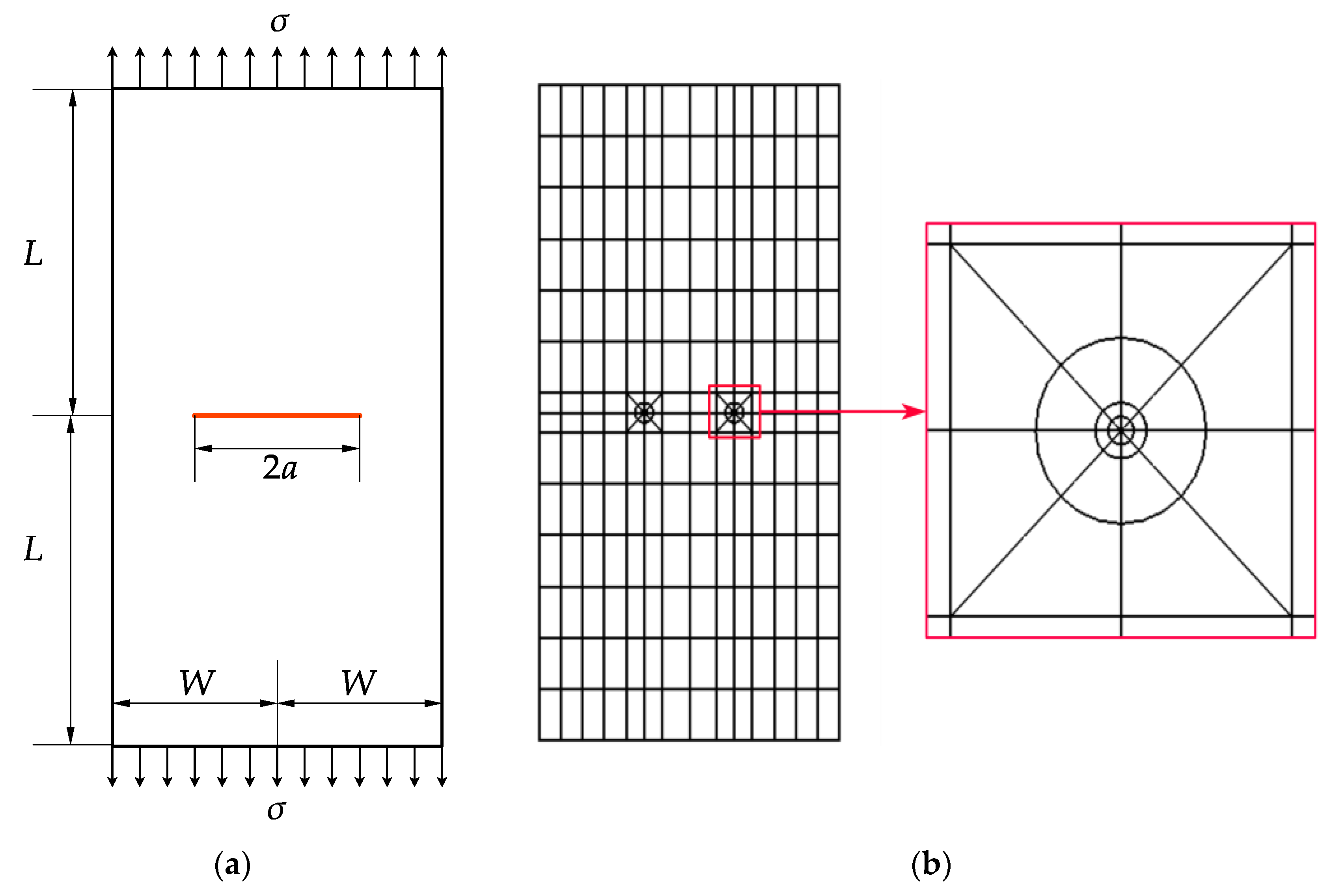
4.4. A Branched Crack in an Infinite Plate
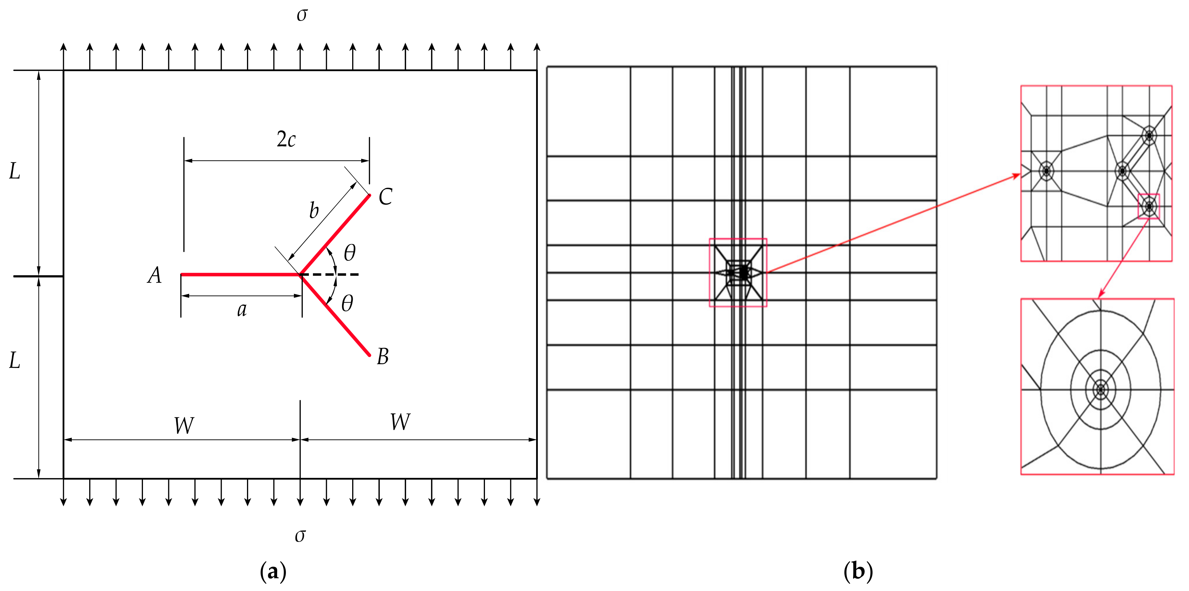
The example is a branched crack in an infinite plate, as shown in Figure 9. A branched cracks embedded in an infinite plate are simulated by the p-version FEM and CIM to demonstrate the accuracy and effectiveness when dealing with complex cracks. Uniform tension unit is applied to the boundary of the plate. The dimensions of the model are , , , and , and the plane stress condition is assumed. The material parameters are considered as Young’s modulus and Poisson’s ratio . The normalized SIFs for crack tips A and C are as follows:
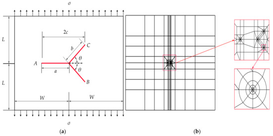
Figure 9.
(a) A branched crack in an infinite plate; (b) Global and local meshes (the total number of elements is 329).
In this example, the normalized SIFs reported in the literature [39] are used as reference solutions. The numerical results obtained by the present method are shown in Table 9, which are compared with the results using the NMM in the literature [40,41] and the reference solutions. It is easy to see that relative error is no more than 0.21% for all the cases, which is less than the relative error in Cai [40,41].
Table 9.
Normalized SIFs for the branched cracks in an infinite plate.
4.5. A Crucifix Crack in a Square Plate under Bi-Axial Tension
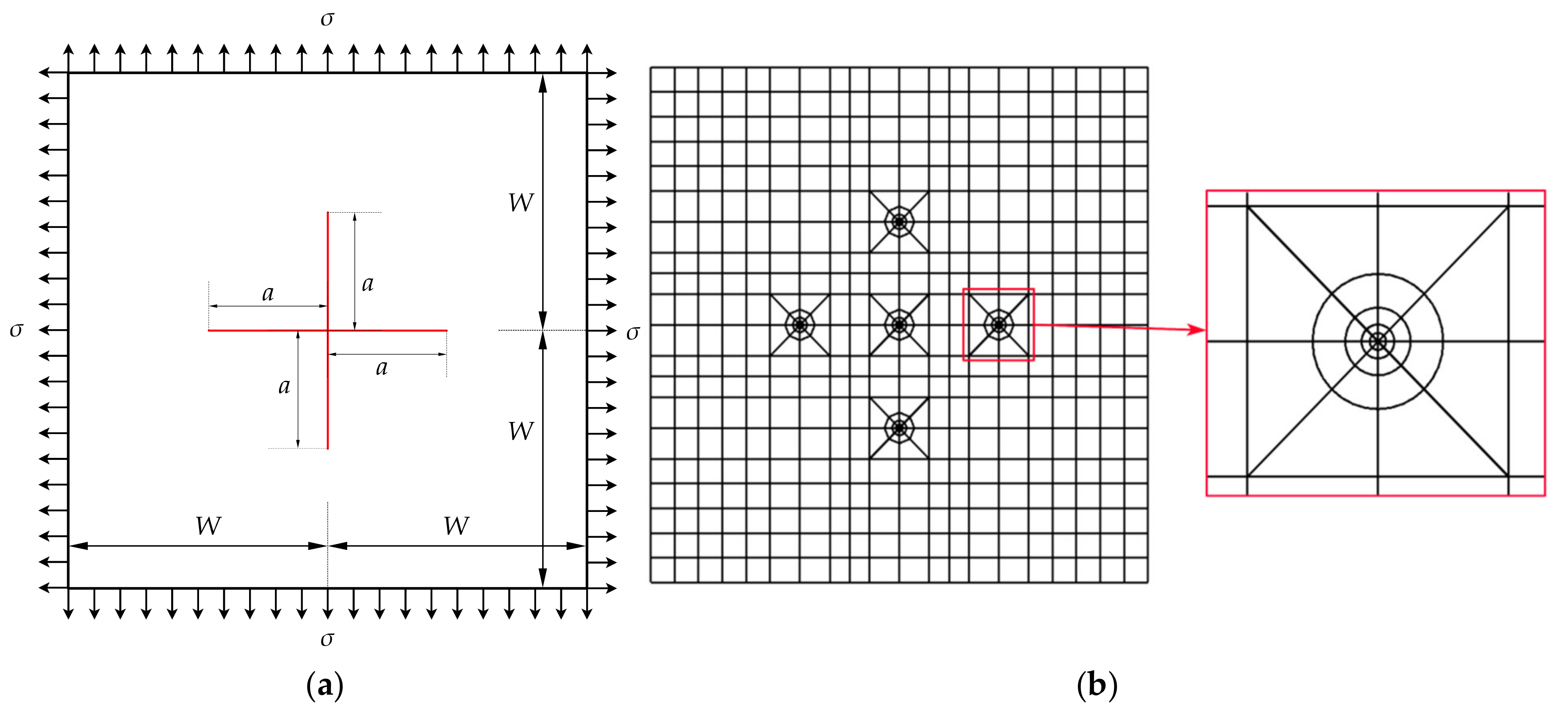
Last example is a crucifix crack in a square plate under bi-axial tension, as shown in Figure 10. The parameters for this example are taken the same as [42,43]: , , , , and the plane strain condition is assumed. Due to symmetry, the SIF at each crack tip is theoretically the same; therefore, only the results at crack tip A are considered. The normalized SIFs and present numerical results comparison with references [42,43] are shown in Table 10.
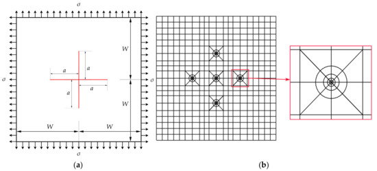
Figure 10.
(a) A crucifix crack in a square plate under bi-axial tension; (b) Global and local meshes (the total number of elements is 580, DOF = 36206).
Table 10.
Normalized SIFs for a crucifix crack.
The computations of SIFs are under the degree of interpolation polynomials p = 1, 2, ..., 8 for all of the examples. Comparisons of the numbers of elements used by different numerical methods are listed in Table 11. In the computations of the first model, the total number of discretizing meshes is 252, and the maximum DOF is 15,678; in the second to the fifth models, the total number of discretizing meshes is 39, 142, 329 and 580, respectively, and the maximum DOF is 2524, 9064, 20,722 and 36,206, respectively. The above examples show that coarse meshes are enough to obtain quite accurate SIFs using the present method. It can be seen that the convergences are very fast with the increasing of degree p from 1 to 8, the accuracy of the SIFs obtained by the present method is also satisfactory, and the SIFs have better stability.
Table 11.
The numbers of elements used for different numerical methods.
5. Conclusions
The SIFs of several classical LEFM models were evaluated based on the P-FEM and CIM, and compared with the results in the literature to verify the effectiveness and accuracy of the present method. The following conclusions can be drawn:
- The computation based on the P-FEM and CIM only needs a fewer number of meshes (less preprocessing), has a faster convergence rate, which can not only be used to analyze the single-crack problems, but also can be used to calculate the SIFs of multiple-crack problems. Furthermore, the present method can also be used to analyze three-dimensional fracture problems and simulate the crack growth path.
- The CIM is a super-convergent method based on the Betti’s theorem of reciprocal works. The SIFs are derived by using the displacements and stresses of higher accuracy on the integral path. Therefore, the CIM can obtain results of relatively higher precision.
- The P-FEM does not need fine meshes, has a faster convergence rate and higher accuracy. However, in the study of crack propagation behavior, it is inevitable to meet the problem of remeshing. On the other hand, the XFEM need not consider the internal geometry of structures and materials; it employs the partition of unity (PU) concept to simulate fracture and crack propagation. The XFEM uses the enrichment functions to reflect the local characteristics of the crack tip and avoids remeshing of meshes. The high-order extended finite element method (high-order XFEM), a combination of the P-FEM with XFEM, will probably have the advantages of both: avoiding remeshing as well as obtaining higher accuracy. The study of the high-order XFEM will be an interesting issue.
Author Contributions
Conceptualization, J.Z.; methodology, J.Z.; software, W.Y. and J.C.; resources, R.X.; Data curation, W.Y.; Funding acquisition, J.Z.; Investigation, J.C.; Validation, W.Y. and R.X.; Writing—original draft, J.Z.; writing—review and editing, W.Y.; visualization, W.Y. and J.C.; supervision, J.Z.; project administration, J.Z.; All authors have read and agreed to the published version of the manuscript.
Funding
This research was funded by the National Natural Science Foundation of China, grant number 51769011.
Institutional Review Board Statement
Not applicable.
Informed Consent Statement
Not applicable.
Data Availability Statement
Data is contained within the present article. Other data presented in this research are available in [6,7,8,37,38,39,40,41,42,43].
Acknowledgments
This research was supported by the National Natural Science Foundation of China (51769011).
Conflicts of Interest
The authors declare no conflict of interest.
References
- Moës, N.; Dolbow, J.; Belytschko, T. A Finite Element Method for Crack Growth without Remeshing. Int. J. Numer. Methods Eng. 1999, 46, 131–150. [Google Scholar] [CrossRef]
- Liu, X.Y.; Xiao, Q.Z.; Karihaloo, B.L. XFEM for Direct Evaluation of Mixed Mode SIFs in Homogeneous and Bi-Materials. Int. J. Numer. Methods Eng. 2004, 59, 1103–1118. [Google Scholar] [CrossRef]
- Dong, Y.W.; Yu, T.T.; Ren, Q.W. Extended Finite Element Method for Direct Evaluation of Strength Intensity Factors. Chin. J. Comput. Mech. 2008, 25, 72–77. [Google Scholar]
- Shouyan, J.; Du Chengbin, G.C.; Xiaocui, C. Computation of Stress Intensity Factors for Interface Cracks between Two Dissimilar Materials Using Extended Finite Element Methods. Eng. Mech. 2015, 32, 22–27. [Google Scholar]
- Su, Y.; Wang, S.; Lu, L. SIFs of Interfacial Crack Using Generalized Extended Finite Element Method. J. Beijing Univ. Aeronaut. Astronaut. 2016, 42, 1162–1168. [Google Scholar] [CrossRef]
- Nianga, J.M.; Mejni, F.; Kanit, T.; Imad, A.; Li, J. Analysis of Crack Parameters under Mixed Mode Loading by Modified Exponential Matrix Method. Theor. Appl. Fract. Mech. 2019, 102, 30–45. [Google Scholar] [CrossRef]
- Liao, M.; Zhang, P. An Improved Approach for Computation of Stress Intensity Factors Using the Finite Element Method. Theor. Appl. Fract. Mech. 2019, 101, 185–190. [Google Scholar] [CrossRef]
- Chen, C.H.; Wang, C.L. Stress Intensity Factors and T-Stresses for Offset Double Edge-Cracked Plates under Mixed-Mode Loadings. Int. J. Fract. 2008, 152, 149–162. [Google Scholar] [CrossRef]
- Cui, X.; Li, H.; Cheng, G.; Tang, C.; Gao, X. Contour Integral Approaches for the Evaluation of Stress Intensity Factors Using Displacement Discontinuity Method. Eng. Anal. Bound. Elem. 2017, 82, 119–129. [Google Scholar] [CrossRef]
- Zhang, J.; Chen, J.; Wu, L. Extraction of Stress Intensity Factors by Using the P-Version Finite Element Method and Contour Integral Method. Acta Mech. Solida Sin. 2020, 33, 836–850. [Google Scholar] [CrossRef]
- Zhang, J.; Xu, R.; He, Y.; Yang, W. Direct Computation of 3-D Stress Intensity Factors of Straight and Curved Planar Cracks with the P-Version Finite Element Method and Contour Integral Method. Materials 2021, 14, 3949. [Google Scholar] [CrossRef]
- Gui, W.; Babuška, I. The h, p Andh-p Versions of the Finite Element Method in 1 Dimension. Numer. Math. 1986, 49, 613–657. [Google Scholar] [CrossRef]
- Babuška, I.; Suri, M. The Optimal Convergence Rate of the P-Version of the Finite Element Method. SIAM J. Numer. Anal. 1987, 24, 750–776. [Google Scholar] [CrossRef]
- Guo, B.; Zhang, J. Stable and Compatible Polynomial Extensions in Three Dimensions and Applications to the p and H-p Finite Element Method. SIAM J. Numer. Anal. 2009, 47, 1195–1225. [Google Scholar] [CrossRef]
- Zhang, Y.; Qiang, S. Research on 3D p-version hierarchical FEM for unsteady temperature field. Rock Soil Mech. 2009, 30, 487–491. [Google Scholar]
- Cheng, Y.; Yu, Z.; Wu, X.; Yuan, Y. Vibration Analysis of a Cracked Rotating Tapered Beam Using the P-Version Finite Element Method. Finite Elem. Anal. Des. 2011, 47, 825–834. [Google Scholar] [CrossRef]
- Stoykov, S.; Ribeiro, P. Vibration Analysis of Rotating 3D Beams by the P-Version Finite Element Method. Finite Elem. Anal. Des. 2013, 65, 76–88. [Google Scholar] [CrossRef]
- Kangsheng, Y.; Zhenwei, Y. A P-Type Superconvergent Recovery Method for FE Analysis of in-Plane Free Vibration of Planar Curved Beams. Eng. Mech. 2019, 36, 28–36. [Google Scholar]
- Farahmand, H.; Ahmadi, A.R.; Arabnejad, S. Thermal Buckling Analysis of Rectangular Microplates Using Higher Continuity P-Version Finite Element Method. Thin-Walled Struct. 2011, 49, 1584–1591. [Google Scholar] [CrossRef]
- Fei, W.; Chen, S. 3-D p-Version Elasto-Viscoplastic Adaptive FEM Model for Hydraulic Structures. J. Hydraul. Eng. 2003, 34, 86–92. [Google Scholar]
- Fei, W.; Chen, S. 3D Steady Seepage Analysis Using p Version Adaptive FEM. ROCK SOIL Mech.-WUHAN- 2004, 25, 211–215. [Google Scholar]
- Yosibash, Z. P-FEMs in Biomechanics: Bones and Arteries. Comput. Methods Appl. Mech. Eng. 2012, 249, 169–184. [Google Scholar] [CrossRef]
- Houmat, A. Three-Dimensional Free Vibration Analysis of Variable Stiffness Laminated Composite Rectangular Plates. Compos. Struct. 2018, 194, 398–412. [Google Scholar] [CrossRef]
- Wu, Y.; Xing, Y.; Liu, B. Hierarchical P-Version C1 Finite Elements on Quadrilateral and Triangular Domains with Curved Boundaries and Their Applications to Kirchhoff Plates. Int. J. Numer. Methods Eng. 2019, 119, 177–207. [Google Scholar] [CrossRef]
- Rahulkumar, P.; Saigal, S.; Yunus, S. Singular P-version finite elements for stress intensity factor computations. Int. J. Numer. Methods Eng. 1997, 40, 1091–1114. [Google Scholar] [CrossRef]
- Munaswamy, K.; Pullela, R. Computation of Stress Intensity Factors for through Cracks in Plates Using P-Version Finite Element Method. Commun. Numer. Methods Eng. 2008, 24, 1753–1780. [Google Scholar] [CrossRef]
- Yu, Z.; Chu, F. Identification of Crack in Functionally Graded Material Beams Using the P-Version of Finite Element Method. J. Sound Vib. 2009, 325, 69–84. [Google Scholar] [CrossRef]
- Wowk, D.; Gamble, K.; Underhill, R. Influence of P-Method Finite Element Parameters on Predictions of Crack Front Geometry. Finite Elem. Anal. Des. 2013, 73, 1–10. [Google Scholar] [CrossRef]
- Wowk, D.; Alousis, L.; Underhill, P.R. An Adaptive Remeshing Technique for Predicting the Growth of Irregular Crack Fronts Using P-Version Finite Element Analysis. Eng. Fract. Mech. 2019, 207, 36–47. [Google Scholar] [CrossRef]
- Szabó, B.; Babuška, I. Introduction to Finite Element Analysis: Formulation, Verification and Validation; John Wiley & Sons: Hoboken, NJ, USA, 2011; ISBN 978-1-119-99348-3. [Google Scholar]
- Pereira, J.P.; Duarte, C.A. The Contour Integral Method for Loaded Cracks. Commun. Numer. Methods Eng. 2006, 22, 421–432. [Google Scholar] [CrossRef]
- Leblanc, A.; Lavie, A. Solving Acoustic Nonlinear Eigenvalue Problems with a Contour Integral Method. Eng. Anal. Bound. Elem. 2013, 37, 162–166. [Google Scholar] [CrossRef]
- Garzon, J.; Duarte, C.A.; Pereira, J.P. Extraction of Stress Intensity Factors for the Simulation of 3-D Crack Growth with the Generalized Finite Element Method. Key Eng. Mater. 2013, 560, 1–36. [Google Scholar] [CrossRef]
- Feng, C.; Li, D.; Gao, S.; Daniel, K. Calculating the Reflected Radiation Error between Turbine Blades and Vanes Based on Double Contour Integral Method. Infrared Phys. Technol. 2016, 79, 171–182. [Google Scholar] [CrossRef]
- Szabo, B.A.; Babuška, I. Computation of the Amplitude of Stress Singular Terms for Cracks and Reentrant Corners. In Fracture Mechanics: Nineteenth Symposium; ASTM International: West Conshohocken, PA, USA, 1988; pp. 101–124. [Google Scholar] [CrossRef]
- Tada, H.; Paris, P.; Irwin, G. The Analysis of Cracks Handbook, 3rd ed.; ASME Press: New York, NY, USA, 2000; ISBN 978-0-7918-0153-6. [Google Scholar]
- Wu, J.; Wang, Y.; Cai, Y.; Ma, G. Direct Extraction of Stress Intensity Factors for Geometrically Elaborate Cracks Using a High-Order Numerical Manifold Method. Eng. Fract. Mech. 2020, 230, 106963. [Google Scholar] [CrossRef]
- Xiao, Q.Z.; Karihaloo, B.L.; Liu, X.Y. Direct Determination of SIF and Higher Order Terms of Mixed Mode Cracks by a Hybrid Crack Element. Int. J. Fract. 2004, 125, 207–225. [Google Scholar] [CrossRef]
- Chen, Y.Z.; Hasebe, N. New Integration Scheme for the Branch Crack Problem. Eng. Fract. Mech. 1995, 52, 791–801. [Google Scholar] [CrossRef]
- Cai, Y.C.; Wu, J.; Atluri, S.N. A New Implementation of the Numerical Manifold Method (NMM) for the Modeling of Non-Collinear and Intersecting Cracks. Comput. Model. Eng. Sci. 2013, 92, 63–85. [Google Scholar]
- Cai, Y.C.; Wu, J. A Robust Algorithm for the Generation of Integration Cells in Numerical Manifold Method. Int. J. Impact Eng. 2016, 90, 165–176. [Google Scholar] [CrossRef]
- Cheung, Y.K.; Woo, C.W.; Wang, Y.H. A General Method for Multiple Crack Problems in a Finite Plate. Comput. Mech. 1992, 10, 335–343. [Google Scholar] [CrossRef]
- Yang, Y.; Xu, D.; Sun, G.; Zheng, H. Modeling Complex Crack Problems Using the Three-Node Triangular Element Fitted to Numerical Manifold Method with Continuous Nodal Stress. Sci. China Technol. Sci. 2017, 60, 1537–1547. [Google Scholar] [CrossRef]
Publisher’s Note: MDPI stays neutral with regard to jurisdictional claims in published maps and institutional affiliations. |
© 2021 by the authors. Licensee MDPI, Basel, Switzerland. This article is an open access article distributed under the terms and conditions of the Creative Commons Attribution (CC BY) license (https://creativecommons.org/licenses/by/4.0/).