Disturbance Observer-Based Chattering-Attenuated Terminal Sliding Mode Control for Nonlinear Systems Subject to Matched and Mismatched Disturbances

Abstract

This work presents a new disturbance observer-based chattering-attenuated terminal sliding mode control for a class of nonlinear systems in the presence of both mismatched and matched disturbances. A nonlinear disturbance observer is typically employed to accurately estimate mismatched disturbances. In this study, a terminal sliding mode control was designed, based on the disturbance estimation results, to counter the effects of disturbances and ultimately stabilize the target system. The utilization of a chattering-attenuated full-order terminal sliding mode structure satisfactorily resolves both chattering and singularity problems in controller design. It was shown by theoretical analyses that both the disturbance estimation error and the system state converge to the equilibrium point in finite time. Two simulation studies, namely a numerical example and an application to an electro hydrostatic actuator system, were conducted to examine the characteristics and to verify the effectiveness of the proposed algorithm.

1. Introduction

Sliding mode control (SMC) is a popular control algorithm and possesses several desirable characteristics, such as design simplicity, ease of implementation, and robustness to external disturbances, model uncertainties, and parameter variations. Thus, SMC has received a significant amount of attention and is widely found in diverse practical applications, including robotics [1,2,3,4,5,6], electrical and mechanical systems [7,8,9,10,11,12], and aerospace engineering [13,14,15,16,17]. Nonetheless, the conventional SMC still exhibits several drawbacks, namely chattering, asymptotic convergence, and susceptibility to mismatched disturbances.

Chattering phenomena occur in the conventional SMC due to the use of a switching function, which leads to high oscillations in the control signal [18]. Significant efforts have been made in the literature to attenuate this problem, including the boundary layer [19], second and higher-order SMC [20,21,22], low-pass filtering [23,24], and the disturbance observer [25]. Another problem found in the conventional SMC is that system states can only asymptotically converge to the equilibrium point. By comparison, terminal sliding mode control (TSMC) can drive system states both to the sliding mode surface and to the equilibrium point in finite time [26]. Although the conventional TSMC inherits the robustness characteristic from its predecessor, it still suffers from the chattering phenomenon and is prone to the singularity problem as the control signal instantly jumps to infinity. A large number of studies have been devoted to solving this problem, e.g., [27,28,29]. Recently, a chattering-free full-order TSMC was developed in [30] that satisfactorily resolves both the chattering and singularity problems mentioned above.

A rather less common problem that SMC faces is mismatched disturbances, which act in a different channel than the control input. Some examples in which mismatched disturbances exist are magnetic levitation (MAGLEV) suspension systems, permanent magnet synchronous motor (PMSM), systems and flight control systems [31]. The various methods that contribute to tackling this problem include integral SMC [32,33,34] and adaptive SMC [35,36,37]. However, it is well known that the integral action may produce several undesirable effects, such as a large overshoot and a long settling time for the control system. Moreover, the nominal performance is normally sacrificed for robustness against disturbances in these methods. Disturbance observer-based SMC, in contrast, is a more promising approach to deal with mismatched disturbances [31,38,39,40,41,42]. In [38], a nonlinear disturbance observer is introduced to develop a new sliding mode surface in an attempt to attenuate mismatched disturbances. However, the mismatched disturbance considered in [38] must be constant rather than time varying, which is a highly restrictive constraint, because the disturbance can continuously change over time in practical applications; that is, unless the mismatched disturbance is time-invariant, the algorithm in [38] fails to stabilize the control system. In addition, the nonlinear disturbance observer utilized in [38] has been proven to be exponentially stable only in the case of slow time-varying mismatched disturbances [43]. A remedy for this constant restriction on the mismatched disturbance formulation is provided in [39], wherein the proposed extended disturbance observer can estimate nonlinear and time-varying mismatched disturbances. However, the problem of being Lyapunov stable without convergence remains, thus limiting the potential of the control algorithm. Another effort to stabilize nonlinear systems is found in [41], where mismatched disturbances are estimated and then suppressed by an extended-state observer-based sliding mode control. Both matched and mismatched disturbances are considered in the paper. Nonetheless, the estimation errors and the system state can only reach and vary in a small region around the equilibrium point, indicating that the observer and the closed-loop system are only Lyapunov stable without convergence. Consequently, the mismatched disturbance cannot be estimated precisely, and the system state cannot be stabilized in finite time.

Motivated by previous works, to accurately estimate and eventually counteract the effect of mismatched disturbances for a class of nonlinear systems, a new design of disturbance observer-based TSMC is introduced in this paper. The finite-time disturbance observer employed in this work originates from an arbitrary-order exact robust differentiator developed in [21]. It forms the basis for the development of this disturbance observer, which has been used by a large number of researchers in various applications. Some of the works are discussed as follows. In [44], the above-mentioned observer is implemented to tackle the tracking control problem of robotic manipulators. In [45], the influence of mismatched disturbances on a class of nonlinear systems is attenuated based on this observer. Simulation of a PMSM then proved the effectiveness of the proposed controller. The same disturbance observer is employed in [46] to address the problem of airgap control of a MAGLEV suspension vehicle. Another application of this disturbance observer can be found in [31], where the authors utilize it to control a DC-DC buck converter. Simulation and experiments on the converter have proven its disturbance rejection capability. These references convincingly demonstrated the effectiveness and the popularity of the disturbance observer considered in the current paper, for estimating and suppressing the influences of matched and mismatched disturbances in different highly nonlinear dynamic systems.

Major aspects of the proposed control algorithm are presented as follows. First, mismatched disturbances are accurately estimated by the nonlinear finite-time disturbance observer. Second, the estimation results are integrated into a new terminal sliding mode surface to enhance system robustness against external disturbances, uncertainties, and unmodeled dynamics. Third, the utilization of a chattering-attenuated full-order terminal sliding mode surface structure in controller design effectively suppresses chattering and singularity phenomena in the control signal. Fourth, Lyapunov stability analysis alongside the design step theoretically increases the reliability of the proposed control scheme. In addition, although the control algorithm is developed for a class of nonlinear second-order systems, the obtained results are extendable to the nth-order formulation. Finally, comparative simulation studies, including a numerical example and an application to an Electro Hydrostatic Actuator (EHA) system, demonstrate the effectiveness of the proposed algorithm.

This work can be perceived to be an extension and improvement of the references [30,41] for several reasons. First, in [30], rigorous research on chattering-free full-order terminal sliding mode control was presented, thus forming the backbone of the development of our work. However, because the control algorithm developed in [30] was only designated to tackle the problem of matched disturbances, it cannot cope with mismatched disturbances, which are more challenging. Second, in [41], an extended-state observer-based sliding mode control (ESOSMC) was introduced in an attempt to address the problem of mismatched disturbances. However, this approach nonetheless exhibited some drawbacks. Although it inherited the chattering attenuation characteristic from the work in [30], the algorithm proposed in [41] was only able to drive the disturbance estimation and system state to a small, bounded region around the equilibrium without actually converging to it. Moreover, the mismatched disturbance used in [41] gradually converged to a constant rather than being time varying throughout the system operation. Thus, the proposal was not practical and was unable to demonstrate the effectiveness of the controller. To address these problems, in this study, a new terminal sliding mode surface was developed. It is enhanced with disturbance rejection by a nonlinear disturbance observer. The proposed control algorithm is expected to suppress both time-varying matched and mismatched disturbances and provide a finite-time convergence characteristic. A brief comparison between the proposed controller and the works presented in [30] and [41] is shown in

Table 1. Comparison of the proposed controller and other works.

Control Algorithm	Matched Disturbance Compensation	Mismatched Disturbance Compensation	Finite-Time Convergence
TSMC [30]	Yes	No	Yes
EOSMC [41]	Yes	Yes	No
The proposed	Yes	Yes	Yes

below.

The remainder of the paper is organized as follows. Section 2 presents the problem formulation. Section 3 introduces the design procedure of the proposed algorithm, followed by stability analysis. Section 4 illustrates the effectiveness of the proposed approach via comparative simulation studies. Ultimately, the conclusion and future work are given in Section 5.

2. Problem Statement

Consider a class of second-order nonlinear systems that are susceptible to both matched and mismatched disturbances as follows [41]:

$$\{\begin{array}{l}{\dot{x}}_1\left(t\right)=x_2\left(t\right)+d_1\left(t\right)\\ {\dot{x}}_2\left(t\right)=f\left(x,t\right)+g\left(x,t\right)u\left(t\right)+d_2\left(t\right)\\ y\left(t\right)=x_1\left(t\right)\end{array}$$

(1)

where $x={\left[x_1,x_2\right]}^T$ is the system state and assumed to be available, $f\left(x,t\right)$ and $g\left(x,t\right)\ne 0$ are two known smooth nonlinear functions, $u\left(t\right)$ is the control input, $y\left(t\right)$ is the system output, and $d_i\left(t\right),\hspace{0.17em}\hspace{0.17em}i=1,2$ are the time-varying mismatched and matched disturbances of the system.

Assumption 1.

Both mismatched and matched disturbances $d_i\left(t\right),\hspace{0.17em}\hspace{0.17em}i=1,2$, and their derivatives, are bounded and satisfy:

$$\begin{array}{ccc}\left|d_i\left(t\right)\right|\le {\varphi }_i,& \left|{\dot{d}}_i\left(t\right)\right|\le {\rho }_i,& i=1,2\end{array}$$

(2)

where ${\varphi }_i>0$and${\rho }_i>0,\hspace{0.17em}\hspace{0.17em}\left(i=1,2\right)$are positive constants. This assumption is reasonably realistic due to the physical limitation of machinery in practical applications.

This work aims to design a disturbance observer-based terminal sliding mode controller to drive the system state $x_1\left(t\right)$ to the origin in finite time in the presence of matched and mismatched disturbances. For this purpose, where the context is sufficiently explicit, the arguments of some functions might be omitted for brevity.

For the system (1), the chattering-free full-order TSMC developed in [30] is derived as below. First, a new terminal sliding mode surface is introduced with the form:

$$s={\dot{x}}_2+c_2{\left|x_2\right|}^{{\alpha }_2}\mathrm{sign}\left(x_2\right)+c_1{\left|x_1\right|}^{{\alpha }_1}\mathrm{sign}\left(x_1\right)$$

(3)

Then, a control law is designed accordingly as:

$$u=g^{-1}\left(x,t\right)\left(u_{eq}+u_n\right)$$

(4)

where $u_{eq}$ denotes the equivalent control and $u_n$ denotes the switching term. The equivalent control $u_{eq}$ is designed as:

$$u_{eq}=-f\left(x,t\right)-c_2{\left|x_2\right|}^{{\alpha }_2}\mathrm{sign}\left(x_2\right)-c_1{\left|x_1\right|}^{{\alpha }_1}\mathrm{sign}\left(x_1\right)$$

(5)

the switching term $u_n$ is defined and filtered by the following method:

$${\dot{u}}_n+T{u}_n=v$$

(6)

$$v=-\left({\rho }_2+k_T+\eta \right)\mathrm{sign}\left(s\right)$$

(7)

where $\eta$ is a positive constant, $T\ge 0$, $k_T$ is chosen satisfying $k_T\ge T{\varphi }_2$, $c_i$ and ${\alpha }_i$ $\left(i=1,2\right)$ are positive constants. $c_i$ can be selected to ensure that the polynomial $p^2+c_{2}p+c_1$ is Hurwitz, and ${\alpha }_i$ can be determined to satisfy [30,47]:

$$\{\begin{array}{l}{\alpha }_1=\frac{{\alpha }_2}{2-{\alpha }_2}\\ {\alpha }_2=\alpha ,\hspace{0.17em}\hspace{0.17em}\alpha \in \left(1-\epsilon ,1\right),\hspace{0.17em}\hspace{0.17em}\epsilon \in \left(0,1\right)\end{array}$$

(8)

By substituting the system (1) and the control law (4) and (5) into the sliding surface (3), one can obtain:

$$\begin{array}{ll}s& ={\dot{x}}_2+c_2{\left|x_2\right|}^{{\alpha }_2}\mathrm{sign}\left(x_2\right)+c_1{\left|x_1\right|}^{{\alpha }_1}\mathrm{sign}\left(x_1\right)\\ & =f\left(x,t\right)+g\left(x,t\right)u+d_2\left(t\right)+c_2{\left|x_2\right|}^{{\alpha }_2}\mathrm{sign}\left(x_2\right)+c_1{\left|x_1\right|}^{{\alpha }_1}\mathrm{sign}\left(x_1\right)\\ & =d_2\left(t\right)+u_n\end{array}$$

(9)

Consider a candidate Lyapunov function of the form: $V\left(s\right)=s^2/2$. It was proven in [48] that the switching term satisfies $\left|u_n\left(t\right)\right|\le {\varphi }_2$. This statement is found to be crucial in proving the finite-time convergence of the sliding surface $s$. Thus, it is re-depicted here for clarity. Initially, $u_n\left(t=0\right)=0$ is taken, i.e., $u_n\left(0\right)\in \left[-{\varphi }_2,{\varphi }_2\right]$. Then, $u_n$ indicates that it cannot leave the interval $\left[-{\varphi }_2,{\varphi }_2\right]$. Recall $\left|d_2\right|\le {\varphi }_2$, $\left|{\dot{d}}_2\right|\le {\rho }_2$ in (2), $k_T\ge T{\varphi }_2$ in the first line after (7), and denote $\beta ={\rho }_2+k_T+\eta$. Due to $s=u_n+d_2$ in (9), (6) can be rewritten as:

$${\dot{u}}_n+T{u}_n=-\beta \mathrm{sign}\left(s\right)=-\beta \mathrm{sign}\left(u_n+d_2\right)$$

(10)

If $u_n>{\varphi }_2$, then $u_n+T{\varphi }_2>0$, $\mathrm{sign}\left(u_n+d_2\right)=\mathrm{sign}\left(u_n\right)=1$. It can be obtained from (10) that:

$${\dot{u}}_n=-T{u}_n-\beta <0$$

Similarly, if $u_n<-{\varphi }_2$, then $\mathrm{sign}\left(u_n+d_2\right)=\mathrm{sign}\left(u_n\right)=-1$. This leads to:

$${\dot{u}}_n=-T{u}_n+\beta >0$$

Thus, the inequality $u_n{\dot{u}}_n<0$ holds outside of $\left[-{\varphi }_2,{\varphi }_2\right]$, and consequently $u_n$ cannot leave $\left[-{\varphi }_2,{\varphi }_2\right]$, i.e., $\left|u_n\right|\le {\varphi }_2$ and, accordingly, $\left|{\dot{d}}_2\left(t\right)+T{u}_n\left(t\right)\right|\le {\rho }_2+T{\varphi }_2$ are retained for any $t\ge 0$. Differentiating the Lyapunov function $V\left(s\right)$ yields:

$$\begin{array}{ll}s\dot{s}& =s\left({\dot{d}}_2+{\dot{u}}_n\right)\\ & =s\left({\dot{d}}_2+\left({\dot{u}}_n+T{u}_n\right)-T{u}_n\right)\\ & =s\left({\dot{d}}_2+v-T{u}_n\right)\\ & \le \left(\left|{\dot{d}}_2-T{u}_n\right|-\left({\rho }_2+k_T+\eta \right)\right)\left|s\right|\\ & =\left(\left|{\dot{d}}_2-T{u}_n\right|-\left({\rho }_2+T{\varphi }_2\right)-\left(k_T-T{\varphi }_2\right)-\eta \right)\left|s\right|\\ & \le -\eta \left|s\right|\end{array}$$

(11)

The inequality (11) indicates that the system states will reach the sliding surface $s=0$ in finite time. Once the desired sliding mode $s=0$ is established, the dynamics of the system can be expressed as:

$$\{\begin{array}{l}{\dot{x}}_1=x_2+d_1\left(t\right)\\ {\dot{x}}_2=-c_2{\left|x_2\right|}^{{\alpha }_2}\mathrm{sign}\left(x_2\right)-c_1{\left|x_1\right|}^{{\alpha }_1}\mathrm{sign}\left(x_1\right)\end{array}$$

(12)

In the case in which there are no mismatched disturbances, (12) becomes:

$$\{\begin{array}{l}{\dot{x}}_1=x_2\\ {\dot{x}}_2=-c_2{\left|x_2\right|}^{{\alpha }_2}\mathrm{sign}\left(x_2\right)-c_1{\left|x_1\right|}^{{\alpha }_1}\mathrm{sign}\left(x_1\right)\end{array}$$

(13)

From (13), if $c_i$ and ${\alpha }_i,\hspace{0.17em}\hspace{0.17em}i=1,2$ are chosen as below (7) and as in (8), respectively, then the system states will converge to the equilibrium in finite time [47,49]. However, in the case in which mismatched disturbances exist, based on the equation set (12), one can obtain the below relationship:

$${\ddot{x}}_1+c_2{\left|{\dot{x}}_1-d_1\right|}^{{\alpha }_2}\mathrm{sign}\left({\dot{x}}_1-d_1\right)+c_1{\left|x_1\right|}^{{\alpha }_1}\mathrm{sign}\left(x_1\right)={\dot{d}}_1$$

(14)

It is clear from the above equation that, despite the control effort, the mismatched disturbance still exists in the system dynamics. Thus, the resulting system state is strongly affected by the mismatched disturbance; that is, although the system state can be attracted to the sliding surface in finite time, it cannot converge to the equilibrium point due to the presence of the time-varying mismatched disturbance. As a result, the chattering-free TSMC developed in [30] can cope with matched disturbances, yet is unable to overcome the influence of mismatched disturbances.

3. Results

In this section, a new chattering-attenuated full-order terminal sliding mode control powered by a nonlinear disturbance observer is proposed for the system (1). First, the disturbance observer is employed to estimate the mismatched disturbance. Subsequently, a new terminal sliding surface and a control law are developed utilizing the estimation results to ensure that the system state converges to the origin in finite time.

3.1. Nonlinear Disturbance Observer

This section aims to employ a finite-time disturbance observer to estimate the time-varying mismatched disturbance existing in (1). Based on the research on globally convergent differentiators in [50], a nonlinear disturbance observer is designed as follows:

$$\{\begin{array}{l}{\dot{z}}_1=v_1+x_2\\ v_1=-{\lambda }_1{L}^{1/3}{\left|z_1-x_1\right|}^{2/3}\mathrm{sign}\left(z_1-x_1\right)-{\mu }_1\left(z_1-x_1\right)+z_2\\ {\dot{z}}_2=v_2\\ v_2=-{\lambda }_2{L}^{1/2}{\left|z_2-v_1\right|}^{1/2}\mathrm{sign}\left(z_2-v_1\right)-{\mu }_2\left(z_2-v_1\right)+z_3\\ {\dot{z}}_3=-{\lambda }_{3}L\mathrm{sign}\left(z_3-v_2\right)-{\mu }_3\left(z_3-v_2\right)\end{array}$$

(15)

where $z_1={\widehat{x}}_1$, $z_2={\widehat{d}}_1$, $z_3={\widehat{\dot{d}}}_1$, and $L>0$, ${\lambda }_i,{\mu }_i>0\hspace{0.17em}\hspace{0.17em}\left(i=1,2,3\right)$.

Assumption 2.

The time-varying mismatched disturbance$d_1\left(t\right)$is assumed to be second-order differentiable and has a Lipschitz constant$L$.

Theorem 1.

Given that the disturbance observer is designed as in (15), if the design parameters are properly selected, the following results can be achieved in finite time:

$$\begin{array}{ccc}{z}_1=x_1,& z_2=d_1,& z_3={\dot{d}}_1\end{array}$$

(16)

Proof of Theorem 1.

For the disturbance observer (15), estimation errors are defined as follows:

$$\begin{array}{ccc}{\epsilon }_1=\frac{z_1-x_1}{L},& {\epsilon }_2=\frac{z_2-d_1}{L},& {\epsilon }_3=\frac{z_3-{\dot{d}}_1}{L}\end{array}$$

(17)

By taking the derivative of ${\epsilon }_1$, ${\epsilon }_2$ and ${\epsilon }_3$, the observer error dynamics can be attained as:

$$\{\begin{array}{l}{\dot{\epsilon }}_1=-{\lambda }_1{\left|{\epsilon }_1\right|}^{2/3}\mathrm{sign}\left({\epsilon }_1\right)-{\mu }_1{\epsilon }_1+{\epsilon }_2\\ {\dot{\epsilon }}_2=-{\lambda }_2{\left|{\epsilon }_2-{\dot{\epsilon }}_1\right|}^{1/2}\mathrm{sign}\left({\epsilon }_2-{\dot{\epsilon }}_1\right)-{\mu }_2\left({\epsilon }_2-{\dot{\epsilon }}_1\right)+{\epsilon }_3\\ {\dot{\epsilon }}_3=-{\lambda }_3\mathrm{sign}\left({\epsilon }_3-{\dot{\epsilon }}_2\right)-{\mu }_3\left({\epsilon }_3-{\dot{\epsilon }}_2\right)-\frac{1}{L}{\ddot{d}}_1\end{array}$$

(18)

Then, according to Theorem 3.1, Lemma B.1, and their proofs in [51], the estimation errors (18) will converge to zero in finite time, indicating that the nonlinear disturbance observer can accurately estimate the system state $x_1\left(t\right)$, the time-varying mismatched disturbance $d_1\left(t\right)$, and its derivative ${\dot{d}}_1\left(t\right)$. This completes the proof of Theorem 1.  □

Remark 1.

Readers are strongly encouraged to inspect the works [21,50,51] and the references therein for better understanding of the rigorous stability analysis of the disturbance observer, and the appropriate selection of its design parameters. It is noted that the observer design parameters, $\left\{{\lambda }_i,{\mu }_i\right\}\left(i=1,2,3\right)$, are chosen recursively in such a manner that$\left\{{\lambda }_i,{\mu }_i\right\}$provide for the convergence of the observer with the Lipschitz constant$L$indicated in Assumption 2. It is also mentioned by the authors that these parameters can be easily changed because the design is not highly sensitive to their values. Nonetheless, the tradeoff is as follows: generally, the greater the parameters, the faster the convergence of the disturbance observer, but the higher the sensitivity to input noises and the sampling step, and the larger the peaking phenomenon in the control signal, if the initial values of the system states and those of the observer states are different. Thus, in the controller design, particularly in the case of different initial values, a tradeoff should be made to ensure fast convergence yet an acceptable peaking phenomenon.

3.2. Disturbance Observer-Based Terminal Sliding Mode Control

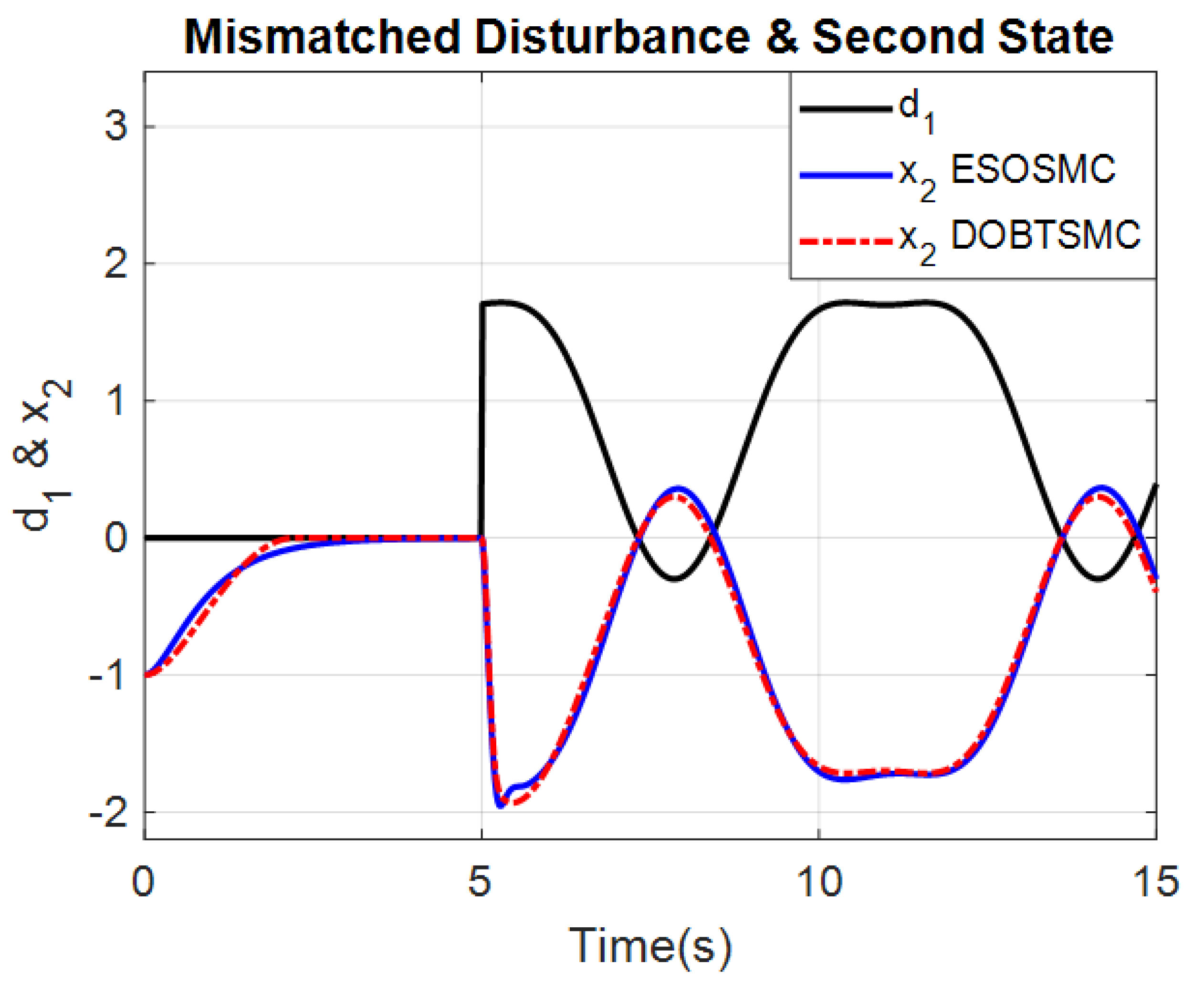
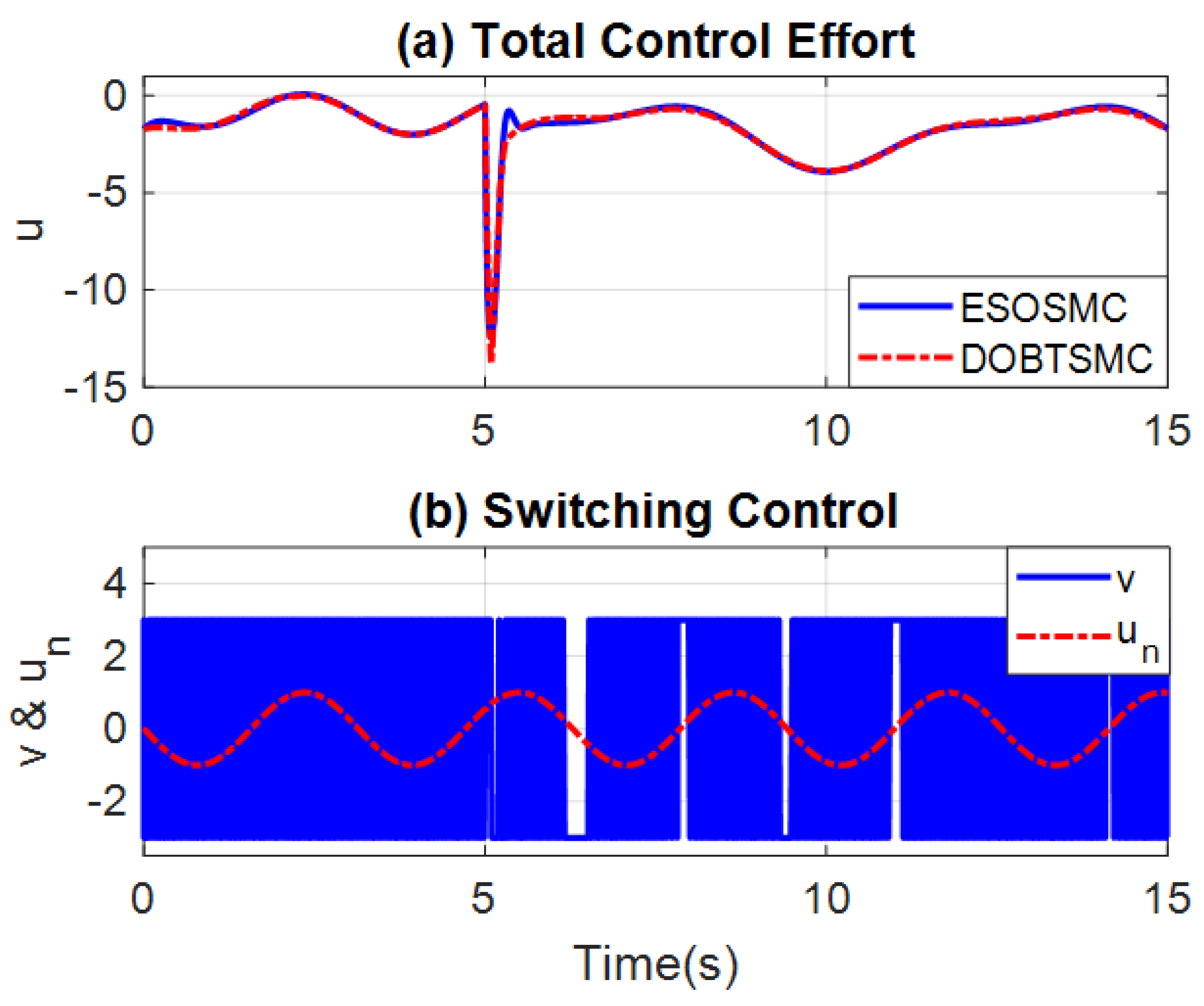
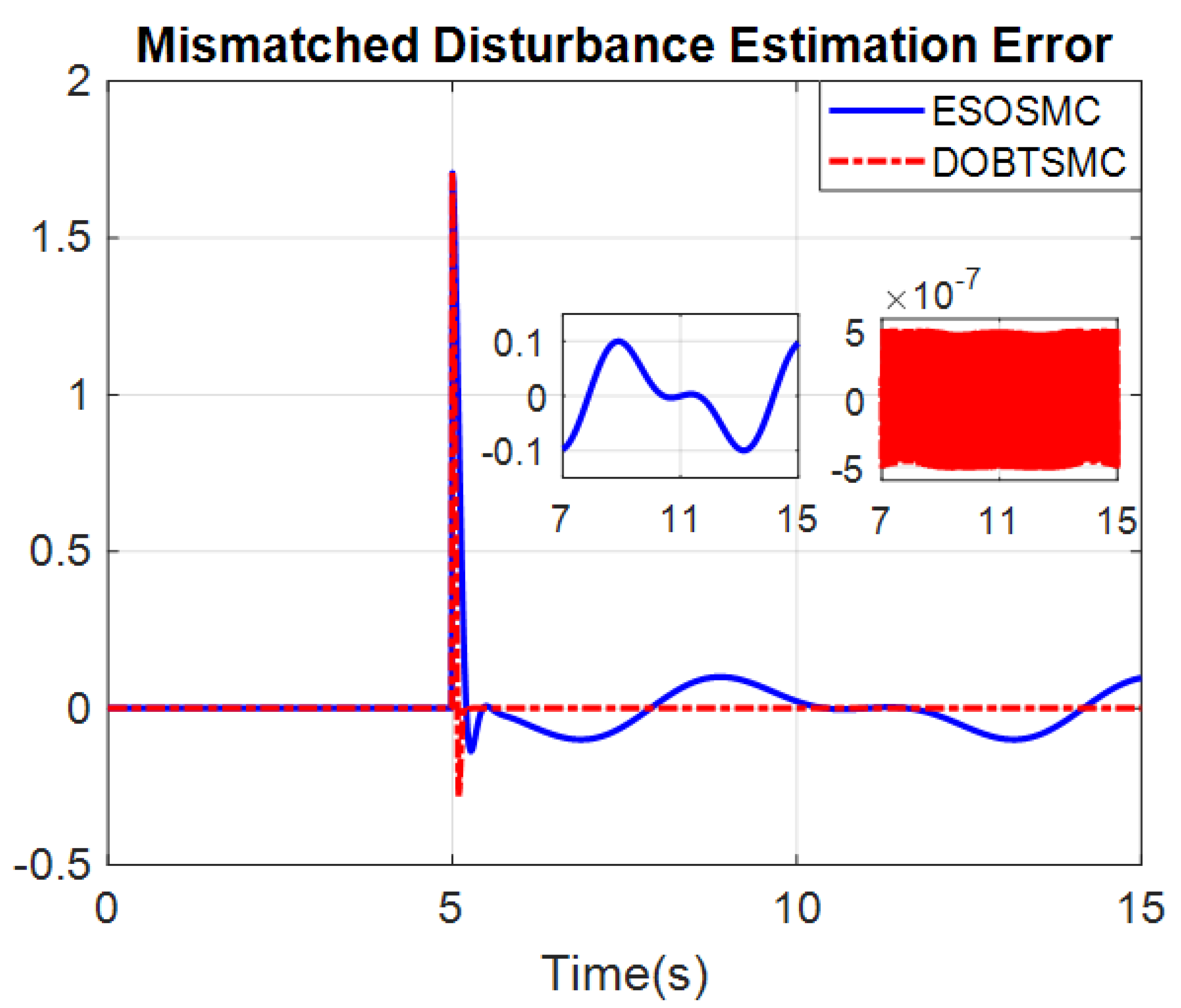
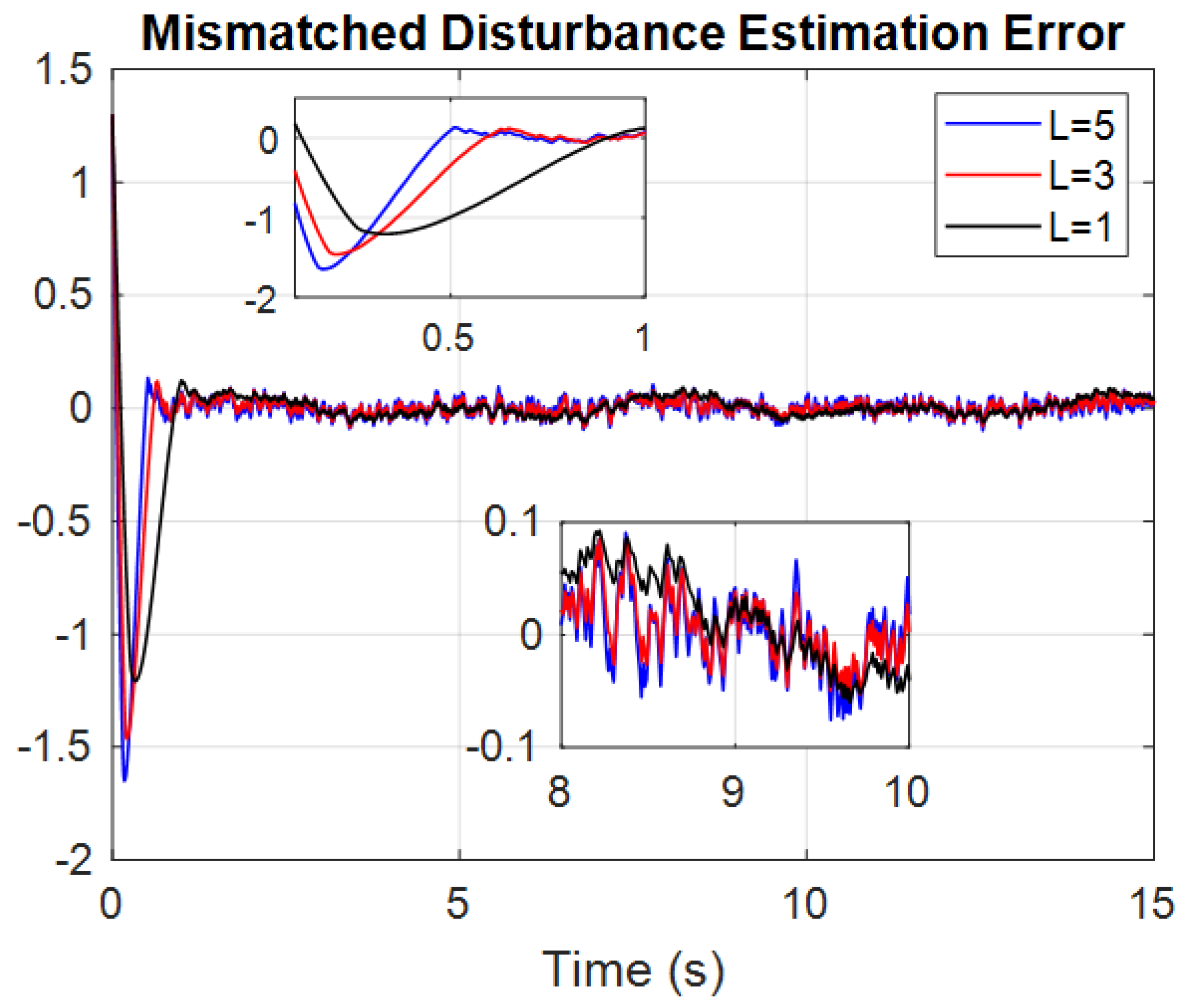
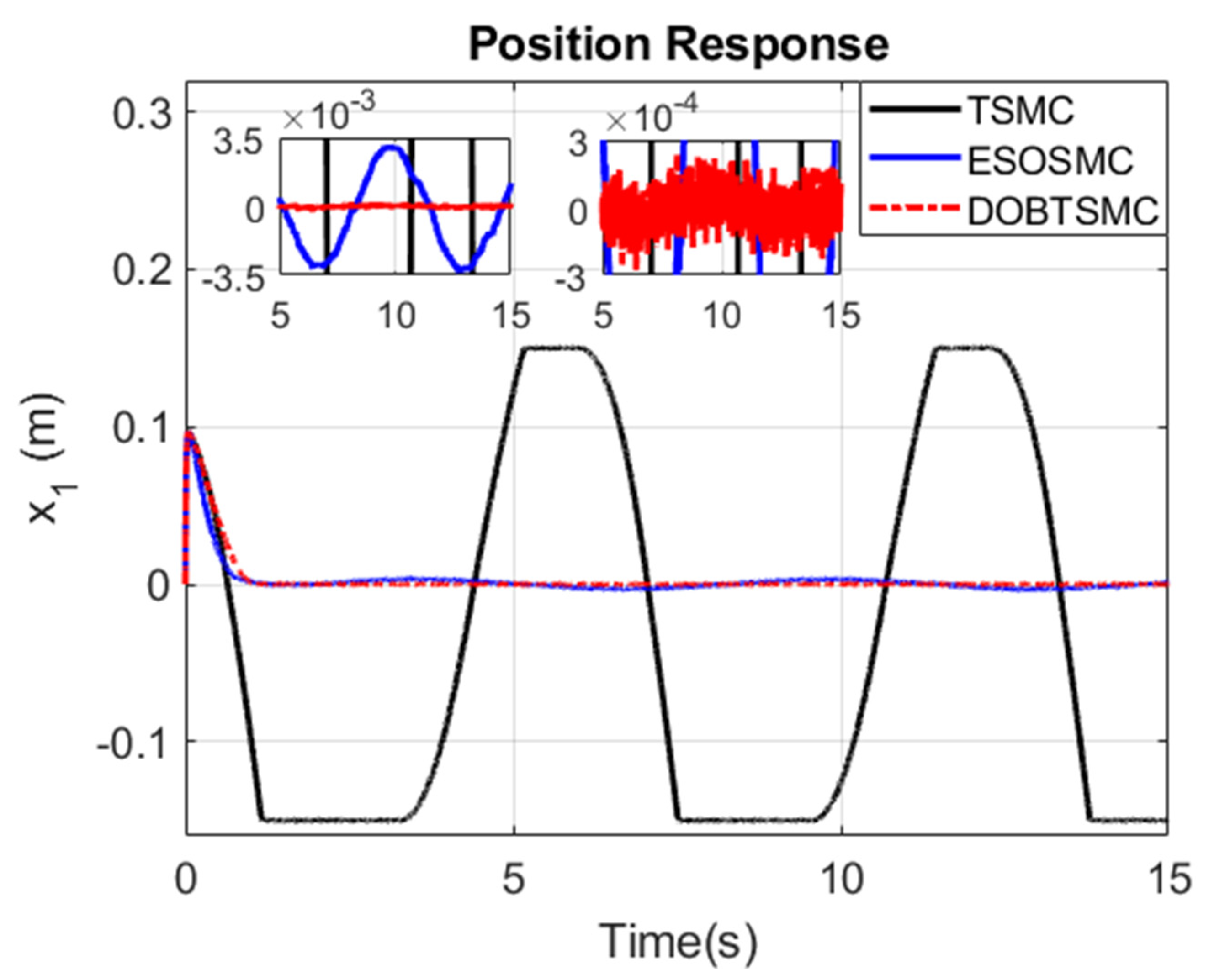
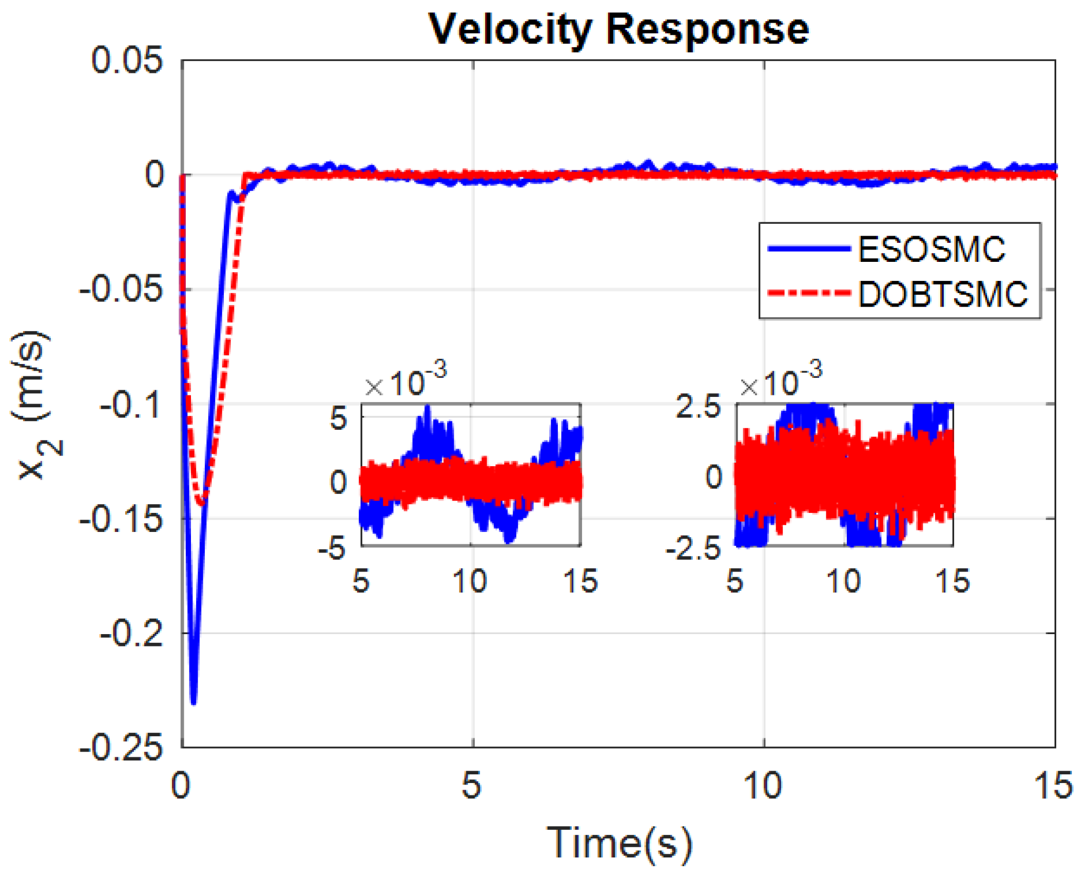
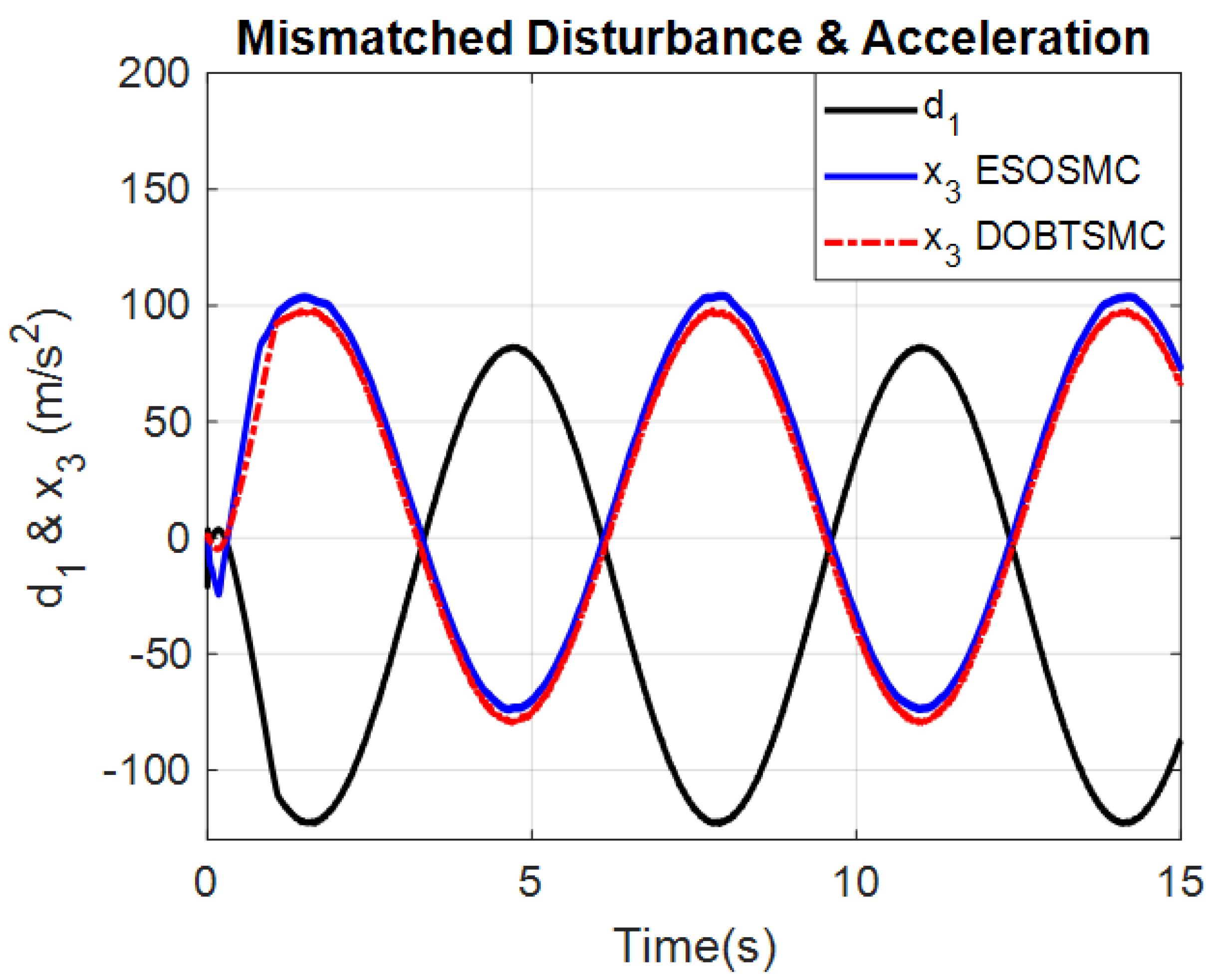
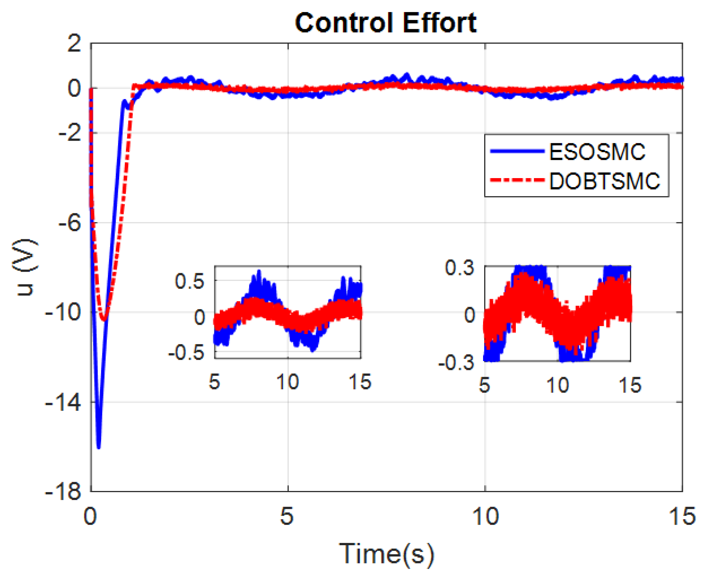
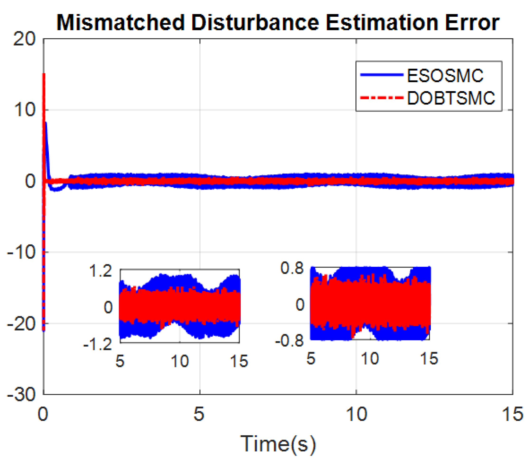
In this section, based on the disturbance estimation, a new sliding surface and, accordingly, a new control law are proposed to drive the system state to the equilibrium point in finite time. This work can be considered as an extension to the control strategy developed in [30] and an improvement of the work [41].

A new disturbance observer (DOB)-based terminal sliding mode surface for the system (1) is proposed as:

$$\sigma ={\dot{x}}_2+c_2{\left|x_2+z_2\right|}^{{\alpha }_2}\mathrm{sign}\left(x_2+z_2\right)+c_1{\left|x_1\right|}^{{\alpha }_1}\mathrm{sign}\left(x_1\right)+z_3$$

(19)

where $z_2={\widehat{d}}_1$, $z_3={\widehat{\dot{d}}}_1$ are obtained from the disturbance observer, and $c_i$ and ${\alpha }_i$ $\left(i=1,2\right)$ are positive constants. $c_i$ are chosen to guarantee that the polynomial $p^2+c_{2}p+c_1$ is Hurwitz, and ${\alpha }_i$ are determined in the same manner as in (8).

Theorem 2.

Given the sliding surface (19), if the control law is developed as:

$$u=g^{-1}\left(x,t\right)\left(u_{eq}+u_n\right)$$

(20)

with the equivalent control:

$$u_{eq}=-f\left(x,t\right)-c_2{\left|x_2+z_2\right|}^{{\alpha }_2}\mathrm{sign}\left(x_2+z_2\right)-c_1{\left|x_1\right|}^{{\alpha }_1}\mathrm{sign}\left(x_1\right)-z_3$$

(21)

and the switching term filtered for chattering attenuation is:

$${\dot{u}}_n+T{u}_n=v$$

(22)

$$v=-\left({\rho }_2+k_T+\eta \right)\mathrm{sign}\left(\sigma \right)$$

(23)

where$T,\hspace{0.17em}\hspace{0.17em}{k}_T,\hspace{0.17em}\hspace{0.17em}\eta \hspace{0.17em}$are defined as same as below (7), then the system (1) will reach the sliding mode surface$\sigma =0$in finite time, and the system state$x_1\left(t\right)$will also converge to the origin in finite time.

Proof of Theorem 2.

By substituting the expression of ${\dot{x}}_2\left(t\right)$ in (1) and the control law (20), (21) into the sliding surface (19), one can derive the following equality:

$$\begin{array}{ll}\sigma & ={\dot{x}}_2+c_2{\left|x_2+z_2\right|}^{{\alpha }_2}\mathrm{sign}\left(x_2+z_2\right)+c_1{\left|x_1\right|}^{{\alpha }_1}\mathrm{sign}\left(x_1\right)+z_3\\ & =\left[f\left(x,t\right)+g\left(x,t\right)u+d_2\left(t\right)\right]+c_2{\left|x_2+z_2\right|}^{{\alpha }_2}\mathrm{sign}\left(x_2+z_2\right)+c_1{\left|x_1\right|}^{{\alpha }_1}\mathrm{sign}\left(x_1\right)+z_3\\ & =d_2\left(t\right)+u_n\end{array}$$

(24)

Consider a candidate Lyapunov function as $V\left(\sigma \right)={\sigma }^2/2$. Differentiating the Lyapunov function $V\left(\sigma \right)$ and following the same procedure in (11) yields:

$$\begin{array}{ll}\dot{V}\left(\sigma \right)& =\sigma \dot{\sigma }\\ & =\sigma \left[{\dot{d}}_2\left(t\right)+{\dot{u}}_n\right]\\ & \le -\eta \left|\sigma \right|\end{array}$$

(25)

which implies that the system will arrive at the sliding surface $\sigma =0$ in finite time. Once the desired sliding mode occurs, combining system (1) and sliding surface (19) yields:

$$\{\begin{array}{l}{\dot{x}}_1=x_2+d_1\\ {\dot{x}}_2=-c_2{\left|x_2+z_2\right|}^{{\alpha }_2}\mathrm{sign}\left(x_2+z_2\right)-c_1{\left|x_1\right|}^{{\alpha }_1}\mathrm{sign}\left(x_1\right)-z_3\end{array}$$

(26)

From the equation set (26), the following relationship can be established:

$$\begin{array}{ll}{\ddot{x}}_1& ={\dot{x}}_2+{\dot{d}}_1\\ & =\left[-c_2{\left|x_2+z_2\right|}^{{\alpha }_2}\mathrm{sign}\left(x_2+z_2\right)-c_1{\left|x_1\right|}^{{\alpha }_1}\mathrm{sign}\left(x_1\right)-z_3\right]+{\dot{d}}_1\\ & =-c_2{\left|\left({\dot{x}}_1-d_1\right)+z_2\right|}^{{\alpha }_2}\mathrm{sign}\left(\left({\dot{x}}_1-d_1\right)+z_2\right)-c_1{\left|x_1\right|}^{{\alpha }_1}\mathrm{sign}\left(x_1\right)-z_3+{\dot{d}}_1\\ & =-c_2{\left|{\dot{x}}_1+\left(z_2-d_1\right)\right|}^{{\alpha }_2}\mathrm{sign}\left({\dot{x}}_1+\left(z_2-d_1\right)\right)-c_1{\left|x_1\right|}^{{\alpha }_1}\mathrm{sign}\left(x_1\right)-\left(z_3-{\dot{d}}_1\right)\end{array}$$

(27)

According to Theorem 1, $z_2=d_1$ and $z_3={\dot{d}}_1$ are achieved in finite time by the disturbance observer. Thus, after the convergence of the disturbance observer, the dynamics (27) become:

$${\ddot{x}}_1=-c_2{\left|{\dot{x}}_1\right|}^{{\alpha }_2}\mathrm{sign}\left({\dot{x}}_1\right)-c_1{\left|x_1\right|}^{{\alpha }_1}\mathrm{sign}\left(x_1\right)$$

(28)

Let $w_1=x_1$, $w_2={\dot{x}}_1$; then, the dynamic Equation (28) can be transformed to:

$$\{\begin{array}{l}{\dot{w}}_1=w_2\\ {\dot{w}}_2=u\end{array}$$

(29)

where $u=-c_2{\left|w_2\right|}^{{\alpha }_2}\mathrm{sign}\left(w_2\right)-c_1{\left|w_1\right|}^{{\alpha }_1}\mathrm{sign}\left(w_1\right)$, and $c_i$, ${\alpha }_i$ $\left(i=1,2\right)$ are designed in the same manner as below equation (19) and equation (8). Then, according to Proposition 8.1 and its proof in [47], it can be concluded that the origin is a globally finite-time-stable equilibrium for the system (29), indicating that the state $x_1\left(t\right)$ of the system (1) will eventually converge to zero in finite time. This completes the proof for Theorem 2.  □

Remark 2.

As stated in [30], the control signal (22) acts in the same manner as a low-pass filter, wherein $\omega =T$ can be interpreted as the bandwidth of the filter. The non-smooth switching function $u_n$ is therefore smoothed to prevent the chattering phenomena from occurring, given that the design parameters have been properly chosen. Moreover, because it is a full-order terminal sliding mode surface, it allows the corresponding control law to be derived without differentiating the term $c_i{|\ast |}^{{\alpha }_i}\mathrm{sign}(\ast )$, thus avoiding the singularity phenomena.

Remark 3.

It should be mentioned that the sliding surface (19) includes the “acceleration” signal${\dot{x}}_2\left(t\right)$, which can be obtained by differentiating the “velocity” signal$x_2\left(t\right)$. Nonetheless, this action is sensitive to noise and thus can degrade system performance. Note that the proposed control law only utilizes the sign of the sliding surface$\sigma$rather than its value. Based on this observation, the same idea suggested in [30] is re-depicted here to avoid the use of the “acceleration” signal. In this approach,$\mathrm{sign}\left(\sigma \right)$can be alternatively determined as follows:

$$\mathrm{sign}\left(\sigma \right)=\mathrm{sign}\left(h\left(t\right)-h\left(t-\tau \right)\right)$$

(30)

where$h\left(t\right)$is defined as:

$$\begin{array}{ll}h\left(t\right)& ={\displaystyle {\int }_0^t\sigma \left(t\right)dt}\\ & =x_2+{\displaystyle {\int }_0^t\left(c_2{\left|x_2+z_2\right|}^{{\alpha }_2}\mathrm{sign}\left(x_2+z_2\right)+c_1{\left|x_1\right|}^{{\alpha }_1}\mathrm{sign}\left(x_1\right)+z_3\right)}dt\end{array}$$

(31)

and$\tau$is chosen to be the fundamental sampling time.

Alternatively, the nonlinear disturbance observer structure can be applied again to meet this need and is presented below:

$$\{\begin{array}{l}{\dot{z}}_4=v_4+x_3\\ v_4=-{\lambda }_4{L}_2{}^{1/3}{\left|z_4-x_2\right|}^{2/3}\mathrm{sign}\left(z_4-x_2\right)-{\mu }_4\left(z_4-x_2\right)+z_5\\ {\dot{z}}_5=v_5\\ v_5=-{\lambda }_5{L}_2{}^{1/2}{\left|z_5-v_4\right|}^{1/2}\mathrm{sign}\left(z_5-v_4\right)-{\mu }_5\left(z_5-v_4\right)+z_6\\ {\dot{z}}_6=-{\lambda }_6{L}_2\mathrm{sign}\left(z_6-v_5\right)-{\mu }_6\left(z_6-v_5\right)\end{array}$$

(32)

where$x_3=f\left(x,t\right)+g\left(x,t\right)u$,$z_4={\widehat{x}}_2$,$z_5={\widehat{d}}_2$,$z_6={\widehat{\dot{d}}}_2$. Because the disturbance observer is proven to be finite-time convergent, after a transient period,${\dot{z}}_4={\dot{\widehat{x}}}_2$can be regarded as the “acceleration” signal. In addition, the matched disturbance$d_2\left(t\right)$can be accurately estimated for further potential, such as reducing the switching gain in the control signal (23), thus decreasing the chance that chattering phenomena will occur. However, the use of another disturbance observer will increase the computational burden, and consequently, a longer response time is expected, which might represent a disadvantage in practice.

Remark 4.

Because the mismatched disturbance is absent from the control system, if the initial values of the observer states are selected as$z_1\left(t_0\right)=x_1\left(t_0\right)$,$z_2\left(t_0\right)=z_3\left(t_0\right)=0$, then it is derived from the observer formulation and observer error dynamics that${\epsilon }_1\left(t\right)={\epsilon }_2\left(t\right)={\epsilon }_3\left(t\right)=0$and$v_1\left(t\right)=v_2\left(t\right)=0$during the absence of mismatched disturbances. In this case, the sliding surface (19) and the control law (20) reduce to those of the conventional TSMC. This indicates the nominal control performance preservation capability of the proposed controller.

Remark 5.

Because the formulation developed earlier in this paper is for second-order systems only, it is desirable to generalize it to an nth-order formulation for different applications. Therefore, the results obtained in this work are extended for a class of nonlinear nth-order systems of the form:

$$\{\begin{array}{l}{\dot{x}}_i=x_{i+1}+d_i\left(t\right),\hspace{0.17em}\hspace{0.17em}\hspace{0.17em}\hspace{0.17em}\hspace{0.17em}\hspace{0.17em}\hspace{0.17em}\hspace{0.17em}i=1,2,\dots ,n-1\\ {\dot{x}}_n=f\left(x,t\right)+g\left(x,t\right)u+d_n\left(t\right)\end{array}$$

(33)

To estimate the mismatched disturbances$d_i\hspace{0.17em}\left(i=1,2,\dots ,n-1\right)$, an nth-order disturbance observer is applied here as follows:

$$\{\begin{array}{l}{\dot{z}}_{1i}=v_{1i}+x_{i+1}={\phi }_{1i}\left(z_{1i}-x_i\right)+z_{2i}+x_{i+1}\\ {\dot{z}}_{2i}=v_{2i}={\phi }_{2i}\left(z_{2i}-v_{1i}\right)+z_{3i}\\ \dots \\ {\dot{z}}_{\left(n+1\right)i}={\phi }_{\left(n+1\right)i}\left(z_{\left(n+1\right)i}-v_{ni}\right)\end{array}$$

(34)

where${\phi }_{ji}$are nonlinear functions of the form:

$${\phi }_{ji}\left(s\right)=-{\lambda }_{ji}{L}_i^{1/\left(n-j+2\right)}{\left|s\right|}^{\left(n-j+1\right)/\left(n-j+2\right)}\mathrm{sign}\left(s\right)-{\mu }_{ji}\left(s\right)$$

(35)

and$z_{1i}={\widehat{x}}_i$,$z_{2i}={\widehat{d}}_i$,$z_{3i}={\widehat{\dot{d}}}_i$,…,$z_{\left(n+1\right)i}=\widehat{d_i{}^{\left(n-1\right)}}$,$L_i>0$,${\lambda }_{ji},{\mu }_{ji}>0$,$j=1,2,\dots ,n+1$. Consequently, an nth-order disturbance observer-based TSMC is designed as:

$$\sigma ={\dot{x}}_n+{\displaystyle {\sum }_{k=2}^n\left(c_k{\left|{\psi }_k\right|}^{{\alpha }_k}\mathrm{sign}\left({\psi }_k\right)\right)}+c_1{\left|x_1\right|}^{{\alpha }_1}\mathrm{sign}\left(x_1\right)+{\chi }_z$$

(36)

where${\psi }_k=x_k+z_{k1}+z_{\left(k-1\right)2}+\dots +z_{2\left(k-1\right)}$,${\chi }_z=z_{3\left(n-1\right)}+z_{4\left(n-2\right)}\dots +z_{\left(n+1\right)1}$. $c_k$and${\alpha }_k$are positive constants such that the polynomial$p^n+{\displaystyle {\sum }_{k=2}^n\left(c_k{p}^{k-1}\right)}+c_1$is Hurwitz and the following equation set is satisfied [30,47]:

$$\{\begin{array}{l}{\alpha }_1=\alpha ,\hspace{0.17em}\hspace{0.17em}\hspace{0.17em}\hspace{0.17em}\hspace{0.17em}\hspace{0.17em}n=1\\ {\alpha }_{k-1}=\frac{{\alpha }_k{\alpha }_{k+1}}{2{\alpha }_{k+1}-{\alpha }_k},\hspace{0.17em}\hspace{0.17em}\hspace{0.17em}\hspace{0.17em}\hspace{0.17em}k=2,\dots ,n\hspace{0.17em}\hspace{0.17em}\hspace{0.17em}\hspace{0.17em}\forall n\ge 2\end{array}$$

(37)

where ${\alpha }_{n+1}=1$, ${\alpha }_n=\alpha$, $\alpha \in \left(1-\epsilon ,1\right)$, $\epsilon \in \left(0,1\right)$.

4. Simulations

In this section, two simulation studies are presented to verify the effectiveness of the control algorithm. Although a numerical example is provided to theoretically assess and discuss the characteristics and performance of the proposed controller, the task of controlling an electro hydrostatic actuator system partly reflects the practicality of the suggested control algorithm. These simulations were conducted in the MATLAB-Simulink environment, wherein the fixed-step ODE4 (Runge–Kutta) was chosen to be the solver. The sampling time was determined separately for each case study, and other settings remained as the defaults.

4.1. Numerical Example

To demonstrate the effectiveness of the proposed control algorithm, the succeeding nonlinear second-order system, which is subject to time-varying mismatched and matched disturbances, is considered:

$$\{\begin{array}{l}{\dot{x}}_1=x_2+d_1\left(t\right)\\ {\dot{x}}_2=-2x_1-x_2+e^{x_1}+u+d_2\left(t\right)\end{array}$$

(38)

Here, the primary objective is to stabilize the above system, and the initial system state is selected away from the equilibrium as $x={\left[1,-1\right]}^T$. Mismatched and matched disturbances are deliberately defined as $d_1\left(t\right)=1+0.3\cos \left(2t\right)-\sin \left(t\right)$ and $d_2\left(t\right)=\sin \left(2t\right)$, respectively. The mismatched disturbance is selected such that as the running time increases and the system state $x_1\left(t\right)$ reaches its steady-state value. The mismatched disturbance is still time varying in a relatively large, bounded region rather than gradually converging to a constant as in the reference [41]. This is a decisive factor in demonstrating the superiority of the proposed control algorithm compared to strategies considered, which will be illustrated by later simulation results. Moreover, to illustrate the nominal control performance preservation characteristic of the proposed control algorithm, the mismatched disturbance is only active after $t=5\hspace{0.17em}\hspace{0.17em}\mathrm{s}$.

For comparison purposes, the chattering-free full-order TSMC approach [30], denoted as TSMC, the extended-state observer-based chattering free SMC [41], denoted as ESOSMC, and the proposed control algorithm, denoted as DOBTSMC, are employed. It should be noted that both DOBTSMC and ESOSMC stem from TSMC, and that the proposed control algorithm, to a certain extent, can be interpreted as an extension and improvement of TSMC and ESOSMC in dealing with mismatched disturbances. Hence, the analogy is drawn here to demonstrate this argument.

Briefly, the ESOSMC proposed in [41] is constructed of a nonlinear extended-state observer (ESO) and an ESO-based SMC. The ESO is designed based on a hyperbolic tangent function of the form:

$$\{\begin{array}{l}{\dot{{\rm Z}}}_1={{\rm Z}}_2-a_1\left({{\rm Z}}_1-x_1\right)+x_2\\ {\dot{{\rm Z}}}_2=-a_2\tanh \left(b\left({{\rm Z}}_1-x_1\right)\right)\end{array}$$

(39)

where ${{\rm Z}}_1={\widehat{x}}_1$, ${{\rm Z}}_2={\widehat{d}}_1$, $\tanh (\ast )=\left(e^{\ast }-e^{-\ast }\right)/\left(e^{\ast }+e^{-\ast }\right)$, $a_i>0$, $i=1,\hspace{0.17em}2$, $b>0$. The sliding mode surface integrated with the ESO is designed as:

$$s={\dot{x}}_2+c_2\left(x_2+{{\rm Z}}_2\right)+c_1{x}_1+{\dot{{\rm Z}}}_2$$

(40)

where $c_i,\hspace{0.17em}\hspace{0.17em}i=1,2$ are chosen in the same manner as in previous sections.

The design control parameters are specifically selected to be the same for all control algorithms as $c_1=5$, $c_2=5$, $T=0.1$, $\left({\rho }_2+k_T+\eta \right)=3$. In addition, for the TSMC and the DOBTSMC, following (8), ${\alpha }_i\left(i=1,2\right)$ are designed as ${\alpha }_1=3/7$, ${\alpha }_2=3/5$. For the mismatched disturbance observers, ESO parameters are selected as $a_1=20$, $a_2=14$ and $b=21$; and DOB parameters are chosen as $L=3$, ${\lambda }_1=6$, ${\lambda }_2=11$, ${\lambda }_3=6$, ${\mu }_1=18$, ${\mu }_2=6$, and ${\mu }_3=2$. The sampling time is set to be $0.1\hspace{0.17em}\hspace{0.17em}\mathrm{ms}$.

The system state $x_1\left(t\right)$ delivered by all control algorithms is shown in Figure 1. For the first $5\hspace{0.17em}\hspace{0.17em}\mathrm{s}$, all controllers are able to stabilize the target system. However, the convergence rate of ESOSMC is lower than that of the other two approaches. It takes ESOSMC about $3.4\hspace{0.17em}\hspace{0.17em}\mathrm{s}$ to reach the 0.01 mark (~1% of the initial value), whereas it takes TSMC and DOBTSMC only around $1.8\hspace{0.17em}\hspace{0.17em}\mathrm{s}$ to reach this mark. Moreover, because the trajectory of TSMC and DOBTSMC are identical in this period, it proves that the proposed control algorithm possesses the nominal performance preservation characteristic in the absence of mismatched disturbances. After $t=5\hspace{0.17em}\hspace{0.17em}\mathrm{s}$, mismatched disturbance starts to affect the control system. It is noticeable that TSMC fails to stabilize the target system, which is already anticipated in the Problem Statement section. Consequently, TSMC signals are suppressed in the following figures for better visualization of other controllers. It can be seen in Figure 1 that, although ESOSMC can only drive the system state to a bounded region of about $0.08$ around the equilibrium, DOBTSMC offers much higher accuracy, with a bound of $[-2.5\times {10}^{-8},\hspace{0.17em}\hspace{0.17em}1.5\times {10}^{-8}]$.

Figure 2 depicts the mismatched disturbance existing in the target system and the second state $x_2\left(t\right)$ response of ESOSMC and DOBTSMC. The figure illustrates that the mismatched disturbance is nonlinear and time varying in a bounded region. It can also be interpreted from the figure that, overall, the trajectory of the mismatched disturbance and that of the second state are symmetric about the horizontal axis 0. This phenomenon can be explained as follows. The system (38) formulation implies that, to stabilize the system state $x_1\left(t\right)$ to the equilibrium point, the following inequality must be fulfilled:

$$\left|{\dot{x}}_1\right|=\left|x_2+d_1\right|\le \delta$$

(41)

where $\delta$ is a sufficiently small positive number and can represent the performance indicator for evaluation. Inequality (41) indicates that for the sake of stabilization, $x_2\left(t\right)$ must counteract the time-varying effect caused by the mismatched disturbance $d_1\left(t\right)$. Consequently, $x_2\left(t\right)$ and $d_1\left(t\right)$ should be opposite. This also explains why the system state $x_1\left(t\right)$ converges to the equilibrium, but not $x_2\left(t\right)$.

Figure 3a records the control signals generated by ESOSMC and the proposed algorithm. It clearly shows that both control signals are smooth without chattering and exhibit the same magnitude of peaking phenomenon at $t=5\hspace{0.17em}\hspace{0.17em}\mathrm{s}$ as the mismatched disturbance is suddenly initiated. The satisfactorily chattering-attenuated control signal results from an attenuation step depicted in Figure 3b, in which the chattering signal $v$ is filtered to create the smooth switching control signal $u_n$, as in (22). Therefore, it demonstrates the effectiveness of the proposed algorithm in attenuating chattering effects.

Figure 4 compares ESOSMC and the proposed control algorithm in mismatched disturbance estimation performance. Under the condition of time-varying mismatched disturbances, from $t=5\hspace{0.17em}\hspace{0.17em}\mathrm{s}$ onwards, the estimation error of ESOSMC varies inside a bounded region of $0.1$ around the equilibrium. In comparison, DOBTSMC can deliver significantly higher precision, with an estimation error of approximately $\pm 5\times {10}^{-7}$. This subsequently contributes to the higher accuracy in the system state response discussed earlier and proves the effectiveness of the proposed controller in mismatched disturbance estimation.

Figure 5 illustrates the sliding surface trajectory of the proposed control algorithm, which oscillates inside the interval $[-0.005;\hspace{0.17em}\hspace{0.17em}0.005]$. Because the sliding surface $\sigma$, defined in (19), is a function of the second state $x_2$, which varies with time to suppress the influence of the mismatched disturbance $d_1$, it is reasonable that the sliding surface $\sigma$ is also time varying. Nonetheless, the proposed control algorithm only utilizes the sign, but not the magnitude, of the sliding surface. Thus, the oscillating trajectory of the sliding surface is believed to have little or no effect on controller performance.

To illustrate the influence of different design parameter values on the performance of the disturbance observer, three simulations were conducted with different values of the Lipschitz constant, $L=1,3,5$. The simulations were carried out in a measurement noise environment with a mean of $0$ and a variance of $5\times {10}^{-3}$, and the sampling time was set to $t_s=0.01\hspace{0.17em}\mathrm{s}$ for practicality. Moreover, the initial values of the observer state and that of the system state were set to be different from each other, ${\widehat{d}}_1\left(0\right)=z_2\left(0\right)=0.5$, $x_1\left(0\right)=1$. The result obtained is shown in Figure 6, which strongly agrees with the statement noted in Remark 1. Specifically, it is evident from Figure 6 that $\left(L=1\right)$ yields the longest convergence time, yet the smallest peaking phenomenon and is least susceptible to noise. In contrast, $\left(L=5\right)$ takes the shortest amount of time for the estimation error to converge to zero but, at the same time, produces the largest peaking phenomenon and is most susceptible to noise. The most appropriate selection is $\left(L=3\right)$, which represents a tradeoff between convergence time and sensitivity to noise and different initial values. Thus, it is concluded here that the greater Lipschitz constant $L$ leads to the faster convergence of the disturbance observer, yet more sensitivity to noise and larger peaking phenomenon in the transition period, especially in case where the initial values of the disturbance observer and the system are different from each other.

4.2. Application to Electro Hydrostatic Actuator System

As presented in this section, the proposed control algorithm developed previously was applied to stabilize an Electro Hydrostatic Actuator (EHA) system.

The EHA studied in this section is illustrated in Figure 7, and the major components are listed in

Table 2. Major components in the considered EHA system.

No.	Device	No.	Device
1	Hydraulic cylinder	5	Directional valve
2	Relief valves	6	Pilot check valve
3	Reservoir	7	Hydraulic pump
4.1	Check valve 4.1	8	AC motor
4.2	Check valve 4.2	9	AC motor driver

. In the hydraulic circuit, cylinder (1) is driven by the valve system and the hydraulic pump (7), which is actuated by the AC motor (8). The flow discrepancy between the bore chamber and the rod chamber of the cylinder is automatically compensated by the check valves (4.1) and (4.2), with the support of the pilot-operated directional valve (5). In cooperation with two pilot-operated check valves (6), the hydraulic pump regulates the fluid flow inside the hydraulic circuit and consequently controls the movement of the cylinder.

Parameters used for mathematical modeling the EHA system are defined in

Table 3. Major components in the considered EHA system.

Symbol	Quantity and Unit
$x$	Displacement of the cylinder. $\left(\mathrm{m}\right)$
$P_1,\hspace{0.17em}{P}_2$	Pressures inside the cylinder chambers. $\left(\mathrm{Pa}\right)$
$A_1,\hspace{0.17em}{A}_2$	Bore- and rod- side areas of the cylinder. $\left({\mathrm{m}}^2\right)$
$m$	Relative mass of the motion system. $\left(\mathrm{kg}\right)$
$V_{10},\hspace{0.17em}{V}_{20}$	Initial volumes of chamber 1 and 2. $\left({\mathrm{m}}^3\right)$
$V_{1t}=V_{10}+A_{1}x$	Active volume of chamber 1. $\left({\mathrm{m}}^3\right)$
$V_{2t}=V_{20}-A_{2}x$	Active volume of chamber 2. $\left({\mathrm{m}}^3\right)$
${\beta }_e$	Effective bulk modulus of the fluid. $\left(\mathrm{Pa}\right)$
$C_{Li}$	Internal leakage coefficient. $\left({\mathrm{m}}^3/\left(\mathrm{sPa}\right)\right)$
$D$	Displacement of the pump. $\left({\mathrm{m}}^3/\mathrm{rad}\right)$
$K_{dr}$	Control gain of the motor driver. $\left(\mathrm{rad}/\left(\mathrm{sV}\right)\right)$
${\eta }_V$	Volumetric efficiency of the pump.
$u$	Driving voltage of the motor driver. $\left(\mathrm{V}\right)$
$b_1,\hspace{0.17em}{b}_2,\hspace{0.17em}{\gamma }_2,\hspace{0.17em}{\gamma }_3$	Positive constants in the system model.
${\delta }_2$	Lumped disturbance in force dynamics. $\left(\mathrm{N}\right)$
${\delta }_{31},\hspace{0.17em}{\delta }_{32}$	Lumped disturbances in pressure dynamics. $\left(\mathrm{N}/\mathrm{s}\right)$

below.

Referring to [52], the dynamic model of the EHA system studied here consists of force dynamics and pressure dynamics, as follows. The force dynamics of the actuator is expressed as:

$$m\ddot{x}=P_1{A}_1-P_2{A}_2+f_{Fr}+{\delta }_2$$

(42)

where ${\delta }_2$ represents a force disturbance that may include external forces and unmodeled force dynamics; $f_{Fr}$ denotes a lumped friction force [53,54] and is approximated as a differential function of the form:

$$\{\begin{array}{l}{f}_{Fr}=-b_1\dot{x}-b_2\tanh \left(\dot{x}\right)\\ \tanh \left(\dot{x}\right)=\frac{1-e^{-{\gamma }_2\dot{x}}}{1+e^{-{\gamma }_2\dot{x}}}\end{array}$$

(43)

Governed by the continuity law [55], the pressure dynamics of the actuator are:

$$\{\begin{array}{c}{V}_{1t}{\dot{P}}_1={\beta }_e\left({\eta }_{V}D{K}_{dr}u-A_1\dot{x}-C_{Li}\left(P_1-P_2\right)-Q_{cv1}\right)+{\delta }_{31}\\ V_{2t}{\dot{P}}_2={\beta }_e\left(-{\eta }_{V}D{K}_{dr}u+A_2\dot{x}+C_{Li}\left(P_1-P_2\right)+Q_{cv2}\right)+{\delta }_{32}\end{array}$$

(44)

where $Q_{cv1}$ and $Q_{cv2}$ are, respectively, the flow in the check valves (4.1) and (4.2), and described as:

$$\{\begin{array}{l}{Q}_{cv1}=-\dot{x}\left(A_1-A_2\right)\mathrm{sm}\left(-\dot{x}\right)\\ Q_{cv2}=\dot{x}\left(A_1-A_2\right)\mathrm{sm}\left(\dot{x}\right)\\ \mathrm{sm}(\ast )={\left(1+e^{-{\gamma }_3\ast }\right)}^{-1}\end{array}$$

(45)

By defining the system state as ${\left[x_1,x_2,x_3\right]}^T={\left[x,\dot{x},\left(P_1{A}_1-P_2{A}_2\right)/m\right]}^T$ and combining equations from (42) to (45), the total dynamic system can be expressed in a canonical form as follows:

$$\{\begin{array}{l}{\dot{x}}_1=x_2\\ {\dot{x}}_2=x_3+d_1\\ {\dot{x}}_3=f+g\hspace{0.17em}u+d_2\end{array}$$

(46)

where the dynamic functions are specifically defined as:

$$\{\begin{array}{l}f=\frac{{\beta }_e}{m}\left[\frac{A_1}{V_{1t}}\left(-A_1+\left(A_1-A_2\right)sm\left(-x_2\right)\right)-\frac{A_2}{V_{2t}}\left(A_2+\left(A_1-A_2\right)sm\left(x_2\right)\right)\right]x_2\\ g=\frac{{\beta }_e{\eta }_{V}D{K}_{dr}}{m}\left(\frac{A_1}{V_{1t}}+\frac{A_2}{V_{2t}}\right)\\ d_1=\frac{1}{m}\left(f_{Fr}+{\delta }_2\right)\\ d_2=-\frac{{\beta }_e}{m}{C}_{Li}\left(P_1-P_2\right)\left(\frac{A_1}{V_{1t}}+\frac{A_2}{V_{2t}}\right)+\frac{A_1{\delta }_{31}}{m{V}_{1t}}-\frac{A_2{\delta }_{32}}{m{V}_{2t}}\end{array}$$

(47)

It can be interpreted from the equation set (46) and (47) that $d_1$, which consists of the lumped friction $f_{Fr}$ and the force disturbance ${\delta }_2$, represents a mismatched disturbance, whereas $d_2$, which includes internal leakages and pressure disturbances, is a matched disturbance. Thus, the EHA system considered here is subject to both mismatched and matched disturbances. It is assumed that these disturbances satisfy Assumptions 1 and 2.

To estimate the mismatched disturbance $d_1$, one can apply (34) to yield a finite-time disturbance observer as follows:

$$\{\begin{array}{l}{\dot{z}}_{12}=v_{12}+x_3\\ v_{12}=-{\lambda }_{12}{L}_2^{1/4}{\left|z_{12}-x_2\right|}^{3/4}\mathrm{sign}\left(z_{12}-x_2\right)-{\mu }_{12}\left(z_{12}-x_2\right)+z_{22}\\ {\dot{z}}_{22}=v_{22}\\ v_{22}=-{\lambda }_{22}{L}_2^{1/3}{\left|z_{22}-v_{12}\right|}^{2/3}\mathrm{sign}\left(z_{22}-v_{12}\right)-{\mu }_{22}\left(z_{22}-v_{12}\right)+z_{32}\\ {\dot{z}}_{32}=v_{32}\\ v_{32}=-{\lambda }_{32}{L}_2^{1/2}{\left|z_{32}-v_{22}\right|}^{1/2}\mathrm{sign}\left(z_{32}-v_{22}\right)-{\mu }_{32}\left(z_{32}-v_{22}\right)+z_{42}\\ {\dot{z}}_{42}=-{\lambda }_{42}{L}_2\mathrm{sign}\left(z_{42}-v_{32}\right)-{\mu }_{42}\left(z_{42}-v_{32}\right)\end{array}$$

(48)

where $z_{12}={\widehat{x}}_2$, $z_{22}={\widehat{d}}_1$, $z_{32}={\widehat{\dot{d}}}_1$, $z_{42}={\widehat{\ddot{d}}}_1$, and $L_2>0$, ${\lambda }_{j2},\hspace{0.17em}{\mu }_{j2}>0\hspace{0.17em}\hspace{0.17em}\left(j=1,\dots ,4\right)$. A chattering-attenuated full-order TSMC for the EHA system can then be designed based on (36) as:

$$\sigma ={\dot{x}}_3+c_3{\left|x_3+z_{22}\right|}^{{\alpha }_3}\mathrm{sign}\left(x_3+z_{22}\right)+c_2{\left|x_2\right|}^{{\alpha }_2}\mathrm{sign}\left(x_2\right)+c_1{\left|x_1\right|}^{{\alpha }_1}\mathrm{sign}\left(x_1\right)+z_{32}$$

(49)

where $c_i$$\left(i=1,2,3\right)$ are positive constants satisfying the requirement that the polynomial $p^3+c_3{p}^2+c_{2}p+c_1$ is Hurwitz, and ${\alpha }_i\left(i=1,2,3\right)$ are chosen as (37). Accordingly, the control law is developed with the form:

$$u=g^{-1}\left(u_{eq}+u_n\right)$$

(50)

where the equivalent control $u_{eq}$ is designed as:

$$u_{eq}=-f-c_3{\left|x_3+z_{22}\right|}^{{\alpha }_3}\mathrm{sign}\left(x_3+z_{22}\right)-c_2{\left|x_2\right|}^{{\alpha }_2}\mathrm{sign}\left(x_2\right)-c_1{\left|x_1\right|}^{{\alpha }_1}\mathrm{sign}\left(x_1\right)-z_{32}$$

(51)

and the switching term $u_n$ is defined as in (22) and (23).

The nominal values of the system parameters were determined as in

Table 4. Nominal values of the EHA system parameters.

Parameter	Unit	Nominal (+ Variance) Value
$m$	$\mathrm{kg}$	$9.32\left(+0.46\right)$
$A_1$	${\mathrm{m}}^2$	$1.9635\times {10}^{-3}\left(+0.0982\times {10}^{-3}\right)$
$A_2$	${\mathrm{m}}^2$	$1.2566\times {10}^{-3}\left(+0.0628\times {10}^{-3}\right)$
$V_{10}$	${\mathrm{m}}^3$	$4.375\times {10}^{-4}\left(+0.219\times {10}^{-4}\right)$
$V_{20}$	${\mathrm{m}}^3$	$2.88\times {10}^{-4}\left(+0.144\times {10}^{-4}\right)$
${\beta }_e$	$\mathrm{Pa}$	$5.34\times {10}^8$
$K_{dr}$	$\mathrm{rad}/\left(\mathrm{sV}\right)$	$10\pi$
$D_1\triangleq {\eta }_{V}D$	${\mathrm{m}}^3/\mathrm{rad}$	$5.83\times {10}^{-7}\left(+0.29\times {10}^{-7}\right)$
$C_{Li}$	${\mathrm{m}}^3/\left(\mathrm{sPa}\right)$	$1.51\times {10}^{-15}$
$b_1$	$\mathrm{Ns}/\mathrm{m}$	$258$
$b_2$	$\mathrm{N}$	$532$
${\gamma }_2$		$10$
$\hspace{0.17em}{\gamma }_3$		$15\left(+0.75\right)$

[56].

The cylinder stroke length is $0.3\hspace{0.17em}\mathrm{m}$; thus, the working range of the actuator is set to be $x_1\in [-0.15,\hspace{0.17em}\hspace{0.17em}0.15]\hspace{0.17em}\mathrm{m}$. For safety purposes, the pressure threshold of the relief valve is set at $150\hspace{0.17em}\mathrm{bar}$, meaning that $P_1,\hspace{0.17em}{P}_2\in [0,\hspace{0.17em}\hspace{0.17em}150\times {10}^5]\hspace{0.17em}\mathrm{Pa}$. To ensure the control task was challenging and to examine the effectiveness of control algorithms, both matched and mismatched disturbances were deliberately assumed to be time varying throughout the simulation period. Specifically, the force disturbance ${\delta }_2$ and the pressure disturbances ${\delta }_{31}$, ${\delta }_{32}$ were selected to be dependent on both time and system state as follows. ${\delta }_2=-1000\left(0.2+0.5x_1+x_2+\sin \left(t\right)\right)$, ${\delta }_{31}=-1000\left(0.1+3x_2+\sin \left(t\right)\right)$, and ${\delta }_{32}=500\left(0.2+x_2+2\sin \left(t\right)\right)$. Moreover, for practicality, measurement noise and parameter uncertainty were added to the simulation. Specifically, the position and pressure measurements were subject to noise with a mean of $0$ and a covariance of $\left\{0.0005\hspace{0.17em}\hspace{0.17em}\mathrm{m},\hspace{0.17em}\hspace{0.17em}3500\hspace{0.17em}\hspace{0.17em}\mathrm{Pa},\hspace{0.17em}\hspace{0.17em}3500\hspace{0.17em}\hspace{0.17em}\mathrm{Pa}\right\}$ [45]. Parameters used to design the controller have nominal values, whereas the parameters used to model the EHA system include variance (~$5\%$ of nominal values), as indicated in Table 4. The sampling time was set to be $1\hspace{0.17em}\hspace{0.17em}\mathrm{ms}$.

Again, the proposed control algorithm, DOBTSMC, was compared with TSMC and ESOSMC in this case study. The design control parameters of DOBTSMC were selected as $c_1=315.6$, $c_2=500$, $c_3=270$; ${\alpha }_i\left(i=1,2,3\right)$ are designed as ${\alpha }_1=1/3$, ${\alpha }_2=1/5$, ${\alpha }_3=1/7$. The DOB parameters were chosen as $L_2=500$, ${\lambda }_{12}=30$, ${\lambda }_{22}=65$, ${\lambda }_{32}=7.5$, ${\lambda }_{42}=5.5$, ${\mu }_{12}=6$, ${\mu }_{22}=13$, ${\mu }_{32}=1.5$, ${\mu }_{42}=1.1$.

Figure 8 presents the position response of the EHA system with the three considered control algorithms, namely, TSMC, ESOSMC, and DOBTSMC. Predictably, TSMC fails to overcome the effects of mismatched disturbances and thus cannot stabilize the target system. It is therefore excluded from the comparison. By comparison, both ESOSMC and DOBTSMC are able to force the system state to remain in the vicinity of the equilibrium. Specifically, the position state $x_1$ generated by ESOSMC varies in a small, bounded region of $3.5\hspace{0.17em}\mathrm{mm}$ around the zero axis. In contrast, the proposed controller, DOBTSMC, provides a much higher precision of about $\pm 0.3\hspace{0.17em}\mathrm{mm}$, which is 10 times more accurate than that of ESOSMC.

The velocity trajectory of ESOSMC and the proposed controller are shown in Figure 9, which shows agreement with the position response in Figure 8. The precision of the DOBTSMC velocity signal, at $\pm 2.3\hspace{0.17em}\mathrm{mm}/\mathrm{s}$, is two-fold higher than that of the ESOSMC velocity signal, at $\pm 5\hspace{0.17em}\mathrm{mm}/\mathrm{s}$. Moreover, a larger peaking phenomenon in the transition period is seen for ESOSMC.

Figure 10 shows the trajectory of the mismatched disturbance and the third state of the control system. It is noticeable that the mismatched disturbance is time varying and that its trajectory and $x_3$ trajectories are symmetric. This phenomenon is consistent with the previous numerical study, where the system state $x_3$ is controlled to cancel out the influence of the mismatched disturbance $d_1$. Thus, $x_3$ and $d_1$ are likely to be opposite in value.

The control signal generated by ESOSMC and the proposed control algorithm are recorded in Figure 11. Overall, both signals are smooth and show few chattering effects. The ESOSMC control signal oscillates inside $\pm 0.5\hspace{0.17em}\mathrm{V}$, whereas the figure for DOBTSMC is slightly better, at $\pm 0.3\hspace{0.17em}\mathrm{V}$. However, ESOSMC exhibits a larger peaking phenomenon than the proposed controller in the transition period.

Figure 12 illustrates the performance of the ESOSMC and that of the proposed controller in estimating mismatched disturbances. The estimation error of DOBTSMC, at about $\pm 0.6\hspace{0.17em}{\mathrm{m}/\mathrm{s}}^2$, is approximately two-fold smaller than that of the ESOSMC, at about $\pm 1.2\hspace{0.17em}{\mathrm{m}/\mathrm{s}}^2$. Both algorithms experience chattering phenomena in the trajectory. This can be explained as follows. Because both schemes utilize system states in observer design, measurement noise in system states has a direct impact on the performance of the observation process. Thus, chattering caused by noise appears and consequently degrades the estimation accuracy of both controllers.

Finally, working pressures of the proposed controller are shown in Figure 13, which clearly implies the nonlinearity of the EHA system. Specifically, the bore chamber area $A_1$ is larger than the rod chamber $A_2$. Thus, to produce the same level of force, the bore chamber pressure $P_1$ must be accordingly smaller than the rod chamber pressure $P_2$. This special condition makes the task of controlling a single rod cylinder much more challenging than the task of controlling a double rod cylinder, where the chamber areas are identical.

5. Conclusions

In this work, a new disturbance observer-based terminal sliding mode control was proposed to control a class of nonlinear systems under the influence of both matched and mismatched disturbances. Although matched disturbances were suppressed by the robust nature of the terminal sliding mode control, mismatched disturbances were compensated by the enhancement in disturbance observation. The employment of a nonlinear disturbance observer enabled the mismatched disturbances to be estimated, and then compensated, by the proposed control algorithm. A general guideline on the appropriate selection of parameters for this observer was provided, and the influence of parameter selection was later illustrated by simulations. Other aspects of the proposed controller, namely, chattering attenuation, sign function utilization, and nominal control performance preservation, were also discussed and demonstrated in this work. Although the proposed control scheme was first designed to stabilize a class of nonlinear second-order systems, it was also shown to be extendable to an nth-order formulation for wider applications. The formulation extension was subsequently used to control a third-order electro hydrostatic actuator system, which, along with a numerical example, revealed the characteristics and verified the effectiveness of the proposed algorithm. Comparative simulation results ultimately demonstrated the satisfactory performance of the proposed controller.

Throughout the study, system states were assumed to be available, and thus different sensors were required. However, there are numerous cases in practice in which only one sensor is implemented for several reasons, such as reducing the installation cost and space. Therefore, future research can be undertaken to design a disturbance-state observer to estimate both disturbances and unmeasured states in a fast-changing, noisy measurement environment.

References

1. Ginoya, D.; Shendge, P.; Phadke, S. Disturbance observer based sliding mode control of nonlinear mismatched uncertain systems. Commun. Nonlinear Sci. Numer. Simul. 2015, 26, 98–107. [Google Scholar] [CrossRef]
2. Jing, C.; Xu, H.; Niu, X. Adaptive sliding mode disturbance rejection control with prescribed performance for robotic manipulators. ISA Trans. 2019, 91, 41–51. [Google Scholar] [CrossRef]
3. Asl, R.M.; Hagh, Y.S.; Palm, R. Robust control by adaptive Non-singular Terminal Sliding Mode. Eng. Appl. Artif. Intell. 2017, 59, 205–217. [Google Scholar] [CrossRef]
4. Ye, H.; Wang, S. Trajectory Tracking Control for Nonholonomic Wheeled Mobile Robots with External Disturbances and Parameter Uncertainties. Int. J. Control Autom. Syst. 2020, 18, 3015–3022. [Google Scholar] [CrossRef]
5. Zhao, Y.; Zhang, Y.; Lee, J. Lyapunov and Sliding Mode Based Leader-follower Formation Control for Multiple Mobile Robots with an Augmented Distance-angle Strategy. Int. J. Control Autom. Syst. 2019, 17, 1314–1321. [Google Scholar] [CrossRef]
6. Jin, Z.; Liang, Z.; Wang, X.; Zheng, M. Adaptive Backstepping Sliding Mode Control of Tractor-trailer System with Input Delay Based on RBF Neural Network. Int. J. Control Autom. Syst. 2020, 19, 76–87. [Google Scholar] [CrossRef]
7. Napole, C.; Barambones, O.; Derbeli, M.; Calvo, I. Advanced Trajectory Control for Piezoelectric Actuators Based on Robust Control Combined with Artificial Neural Networks. Appl. Sci. 2021, 11, 7390. [Google Scholar] [CrossRef]
8. Gao, Y.; Wu, Y.; Wang, X.; Chen, Q. Characteristic Model-based Adaptive Control with Genetic Algorithm Estimators for Four-PMSM Synchronization System. Int. J. Control Autom. Syst. 2020, 18, 1605–1616. [Google Scholar] [CrossRef]
9. Wang, J.; Zhao, L.; Yu, L. Reduced-order Generalized Proportional Integral Observer Based Continuous Dynamic Sliding Mode Control for Magnetic Levitation System with Time-varying Disturbances. Int. J. Control Autom. Syst. 2020, 19, 439–448. [Google Scholar] [CrossRef]
10. Din, S.U.; Khan, Q.; Rehman, F.U.; Akmeliawanti, R. A Comparative Experimental Study of Robust Sliding Mode Control Strategies for Underactuated Systems. IEEE Access 2017, 6, 1927–1939. [Google Scholar] [CrossRef]
11. Derbeli, M.; Barambones, O.; Silaa, M.; Napole, C. Real-Time Implementation of a New MPPT Control Method for a DC-DC Boost Converter Used in a PEM Fuel Cell Power System. Actuators 2020, 9, 105. [Google Scholar] [CrossRef]
12. Napole, C.; Derbeli, M.; Barambones, O. A global integral terminal sliding mode control based on a novel reaching law for a proton exchange membrane fuel cell system. Appl. Energy 2021, 301, 117473. [Google Scholar] [CrossRef]
13. Chen, Z.; Tu, X.; Xing, L.; Fu, J.; Lozano, R.; Rogelio, L. A Special Kind of Sliding Mode Control for Nonlinear System with State Constraints. IEEE Access 2019, 7, 69998–70010. [Google Scholar] [CrossRef]
14. Kamalesh, M.; Senthilnathan, N.; Bharatiraja, C. Design of a Novel Boomerang Trajectory for Sliding Mode Controller. Int. J. Control Autom. Syst. 2020, 18, 2917–2928. [Google Scholar] [CrossRef]
15. Ye, D.; Zhang, H.; Tian, Y.; Zhao, Y.; Sun, Z. Fuzzy Sliding Mode Control of Nonparallel-ground-track Imaging Satellite with High Precision. Int. J. Control Autom. Syst. 2020, 18, 1617–1628. [Google Scholar] [CrossRef]
16. Xu, S.S.-D.; Chen, C.-C.; Wu, Z.-L. Study of Nonsingular Fast Terminal Sliding-Mode Fault-Tolerant Control. IEEE Trans. Ind. Electron. 2015, 62, 3906–3913. [Google Scholar] [CrossRef]
17. Feng, Y.; Zhou, M.; Zheng, X.; Han, F.; Yu, X. Full-order terminal sliding-mode control of MIMO systems with unmatched uncertainties. J. Frankl. Inst. 2018, 355, 653–674. [Google Scholar] [CrossRef]
18. Levant, A. Chattering Analysis. IEEE Trans. Autom. Control 2010, 55, 1380–1389. [Google Scholar] [CrossRef]
19. Kachroo, P.; Tomizuka, M. Chattering reduction and error convergence in the sliding-mode control of a class of nonlinear systems. IEEE Trans. Autom. Control 1996, 41, 1063–1068. [Google Scholar] [CrossRef] [Green Version]
20. Bartolini, G.; Ferrara, A.; Usai, E. Chattering avoidance by second-order sliding mode control. IEEE Trans. Autom. Control 1998, 43, 241–246. [Google Scholar] [CrossRef]
21. Levant, A. Higher-order sliding modes, differentiation and output-feedback control. Int. J. Control 2003, 76, 924–941. [Google Scholar] [CrossRef]
22. Levant, A. Principles of 2-sliding mode design. Automatica 2007, 43, 576–586. [Google Scholar] [CrossRef] [Green Version]
23. Xu, J.-X.; Pan, Y.-J.; Lee, T.-H. Sliding Mode Control with Closed-Loop Filtering Architecture for a Class of Nonlinear Systems. IEEE Trans. Circuits Syst. II Express Briefs 2004, 51, 168–173. [Google Scholar] [CrossRef]
24. Tseng, M.-L.; Chen, M.-S. Chattering reduction of sliding mode control by low-pass filtering the control signal. Asian J. Control 2010, 12, 392–398. [Google Scholar] [CrossRef]
25. Kawamura, A.; Itoh, H.; Sakamoto, K. Chattering reduction of disturbance observer based sliding mode control. IEEE Trans. Ind. Appl. 1994, 30, 456–461. [Google Scholar] [CrossRef]
26. Mu, C.; He, H. Dynamic Behavior of Terminal Sliding Mode Control. IEEE Trans. Ind. Electron. 2017, 65, 3480–3490. [Google Scholar] [CrossRef]
27. Corradini, M.L.; Cristofaro, A. Nonsingular terminal sliding-mode control of nonlinear planar systems with global fixed-time stability guarantees. Automatica 2018, 95, 561–565. [Google Scholar] [CrossRef]
28. Rabiee, H.; Ataei, M.; Ekramian, M. Continuous nonsingular terminal sliding mode control based on adaptive sliding mode disturbance observer for uncertain nonlinear systems. Automatica 2019, 109, 108515. [Google Scholar] [CrossRef]
29. Wang, Y.; Zhu, K.; Yan, F.; Chen, B. Adaptive super-twisting nonsingular fast terminal sliding mode control for cable-driven manipulators using time-delay estimation. Adv. Eng. Softw. 2018, 128, 113–124. [Google Scholar] [CrossRef]
30. Feng, Y.; Han, F.; Yu, X. Chattering free full-order sliding-mode control. Automatica 2014, 50, 1310–1314. [Google Scholar] [CrossRef]
31. Wang, J.; Li, S.; Yang, J.; Wu, B.; Li, Q. Finite-time disturbance observer based non-singular terminal sliding-mode control for pulse width modulation based DC–DC buck converters with mismatched load disturbances. IET Power Electron. 2016, 9, 1995–2002. [Google Scholar] [CrossRef]
32. Utkin, V.; Shi, J. Integral sliding mode in systems operating under uncertainty conditions. In Proceedings of the 35th IEEE Conference on Decision and Control, Las Vegas, NV, USA, 13 December 2002; Volume 4, pp. 4591–4596. [Google Scholar] [CrossRef]
33. Cao, W.-J.; Xu, J.-X. Nonlinear Integral-Type Sliding Surface for Both Matched and Unmatched Uncertain Systems. IEEE Trans. Autom. Control 2004, 49, 1355–1360. [Google Scholar] [CrossRef]
34. Castanos, F.; Fridman, L. Analysis and Design of Integral Sliding Manifolds for Systems With Unmatched Perturbations. IEEE Trans. Autom. Control 2006, 51, 853–858. [Google Scholar] [CrossRef] [Green Version]
35. Mondal, S.; Mahanta, C. Chattering free adaptive multivariable sliding mode controller for systems with matched and mismatched uncertainty. ISA Trans. 2013, 52, 335–341. [Google Scholar] [CrossRef]
36. Kwan, C.-M. Sliding mode control of linear systems with mismatched uncertainties. Automatica 1995, 31, 303–307. [Google Scholar] [CrossRef]
37. Wen, C.-C.; Cheng, C.-C. Design of sliding surface for mismatched uncertain systems to achieve asymptotical stability. J. Frankl. Inst. 2008, 345, 926–941. [Google Scholar] [CrossRef]
38. Yang, J.; Li, S.; Yu, X. Sliding-Mode Control for Systems with Mismatched Uncertainties via a Disturbance Observer. IEEE Trans. Ind. Electron. 2012, 60, 160–169. [Google Scholar] [CrossRef]
39. Ginoya, D.; Shendge, P.D.; Phadke, S. Sliding Mode Control for Mismatched Uncertain Systems Using an Extended Disturbance Observer. IEEE Trans. Ind. Electron. 2013, 61, 1983–1992. [Google Scholar] [CrossRef]
40. Zhang, J.; Liu, X.; Xia, Y.; Zuo, Z.; Wang, Y. Disturbance Observer-Based Integral Sliding-Mode Control for Systems with Mismatched Disturbances. IEEE Trans. Ind. Electron. 2016, 63, 7040–7048. [Google Scholar] [CrossRef]
41. Shi, S.-L.; Li, J.-X.; Fang, Y. Extended-State-Observer-Based Chattering Free Sliding Mode Control for Nonlinear Systems with Mismatched Disturbance. IEEE Access 2018, 6, 22952–22957. [Google Scholar] [CrossRef]
42. Nguyen, N.P.; Oh, H.; Kim, Y.; Moon, J. Disturbance Observer-Based Continuous Finite-Time Sliding Mode Control against Matched and Mismatched Disturbances. Complexity 2020, 2020, 1–14. [Google Scholar] [CrossRef]
43. Chen, W.-H. Nonlinear Disturbance Observer-Enhanced Dynamic Inversion Control of Missiles. J. Guid. Control Dyn. 2003, 26, 161–166. [Google Scholar] [CrossRef]
44. Su, J.; Yang, J.; Li, S. Continuous finite-time anti-disturbance control for a class of uncertain nonlinear systems. Trans. Inst. Meas. Control 2013, 36, 300–311. [Google Scholar] [CrossRef]
45. Yang, J.; Li, S.; Su, J.; Yu, X. Continuous nonsingular terminal sliding mode control for systems with mismatched disturbances. Automatica 2013, 49, 2287–2291. [Google Scholar] [CrossRef] [Green Version]
46. Yang, J.; Su, J.; Li, S.; Yu, X. High-Order Mismatched Disturbance Compensation for Motion Control Systems Via a Continuous Dynamic Sliding-Mode Approach. IEEE Trans. Ind. Inform. 2013, 10, 604–614. [Google Scholar] [CrossRef] [Green Version]
47. Bhat, S.P.; Bernstein, D.S. Geometric homogeneity with applications to finite-time stability. Math. Control Signals Syst. 2005, 17, 101–127. [Google Scholar] [CrossRef] [Green Version]
48. Feng, Y.; Han, F.; Yu, X. Reply to “Comments on ‘Chattering free full-order sliding-mode control’ [Automatica 50 (2014) 1310–1314]”. Automatica 2016, 72, 255–256. [Google Scholar] [CrossRef]
49. Bhat, S.; Bernstein, D. Finite-time stability of homogeneous systems. In Proceedings of the 1997 American Control Conference (Cat. No.97CH36041), Albuquerque, NM, USA, 6 June 1997. [Google Scholar] [CrossRef]
50. Levant, A.; Livne, M. Globally convergent differentiators with variable gains. Int. J. Control 2018, 91, 1994–2008. [Google Scholar] [CrossRef]
51. Levant, A. Homogeneity approach to high-order sliding mode design. Automatica 2005, 41, 823–830. [Google Scholar] [CrossRef]
52. Ba, D.X.; Dinh, T.Q.; Bae, J.; Ahn, K.K. An Effective Disturbance-Observer-Based Nonlinear Controller for a Pump-Controlled Hydraulic System. IEEE/ASME Trans. Mechatron. 2019, 25, 32–43. [Google Scholar] [CrossRef]
53. Yao, J.; Jiao, Z.; Ma, D.; Yan, L. High-Accuracy Tracking Control of Hydraulic Rotary Actuators with Modeling Uncertainties. IEEE/ASME Trans. Mechatron. 2013, 19, 633–641. [Google Scholar] [CrossRef]
54. Won, D.; Kim, W.; Shin, D.; Chung, C.C. High-Gain Disturbance Observer-Based Backstepping Control With Output Tracking Error Constraint for Electro-Hydraulic Systems. IEEE Trans. Control Syst. Technol. 2014, 23, 787–795. [Google Scholar] [CrossRef]
55. Merritt, H.E.; Pomper, V. Hydraulic control systems. J. Appl. Mech. 1968, 35, 200. [Google Scholar] [CrossRef]
56. Ba, D.X.; Ahn, K.K.; Truong, D.Q.; Park, H.G. Integrated model-based backstepping control for an electro-hydraulic system. Int. J. Precis. Eng. Manuf. 2016, 17, 565–577. [Google Scholar] [CrossRef]
Figure 1. Response trajectory of the state x 1
Applsci 11 08158 g001
Figure 2. Mismatched disturbance and second state response trajectories.
Applsci 11 08158 g002
Figure 3. Total control signal (a) and switching control signal (b).
Applsci 11 08158 g003
Figure 4. Mismatched disturbance estimation error of ESOSMC and DOBTSMC.
Applsci 11 08158 g004
Figure 5. Sliding surface response of the proposed control algorithm.
Applsci 11 08158 g005
Figure 6. Influence of design parameters on observer performance.
Applsci 11 08158 g006
Figure 7. Schematic diagram of the studied EHA system.
Applsci 11 08158 g007
Figure 8. Position response of the EHA system.
Applsci 11 08158 g008
Figure 9. Velocity response of the EHA system.
Applsci 11 08158 g009
Figure 10. Mismatched disturbance and acceleration signal of the EHA system.
Applsci 11 08158 g010
Figure 11. Control signal trajectory of ESOSMC and DOBTSMC.
Applsci 11 08158 g011
Figure 12. Mismatched disturbance estimation error of ESOSMC and DOBTSMC.
Applsci 11 08158 g012
Figure 13. Working pressures of the proposed controller.
Applsci 11 08158 g013