Abstract
Mild cognitive impairment (MCI) is an indicative precursor of Alzheimer’s disease and its early detection is critical to restrain further cognitive deterioration through preventive measures. In this context, the capacity of serious games combined with machine learning for MCI detection is examined. In particular, a custom methodology is proposed, which consists of a series of steps to train and evaluate classification models that could discriminate healthy from cognitive impaired individuals on the basis of game performance and other subjective data. Such data were collected during a pilot evaluation study of a gaming platform, called COGNIPLAT, with 10 seniors. An exploratory analysis of the data is performed to assess feature selection, model overfitting, optimization techniques and classification performance using several machine learning algorithms and standard evaluation metrics. A production level model is also trained to deal with the issue of data leakage while delivering a high detection performance (92.14% accuracy, 93.4% sensitivity and 90% specificity) based on the Gaussian Naive Bayes classifier. This preliminary study provides initial evidence that serious games combined with machine learning methods could potentially serve as a complementary or an alternative tool to the traditional cognitive screening processes.
1. Introduction
Studies have shown that the cognitive functions of the elderly are negatively affected by a number of factors, such as heredity, lifestyle (e.g., diet, smoking, alcohol), and age-related pathological conditions [1]. With regard to normal aging, it appears that many cognitive functions remain stable throughout life with mild attenuation beginning gradually in the sixth or seventh decade of life [2]. Mild cognitive impairment (MCI) is often labeled as a precursor of dementia and especially of Alzheimer’s disease (AD) [3] or just as an intermediate level of cognitive function that is lower compared to what is considered normal for a certain age and an educational level [4].
The current approach of MCI diagnosis is through a clinical check-up, performed by a specialist, that includes an interview with the subject, the collection of the subject’s medical history, a series of neurological examinations to test the mobility, the balance, the functionality of the nervous system and finally a cognitive assessment, such as the Mini Mental State Examination (MMSE) [5] or the Montreal Cognitive Assessment (MoCA) [6]. Although this approach provides the specialist with a wealth of information, beyond an assessment score, which is assistive in drawing safe conclusions about the cognitive level of the subject, it also presents some disadvantages. Given that the assessment is part of a clinical check-up, the potential anxiety of the subject along with other convoluted factors might result in a decreased performance. This situation combined with the low repeatability of the clinical check-ups may lead to distorted assessments [7].
An aspect of the MCI detection is the stage at which it is performed. According to a research that was conducted with a cohort of 139 subjects and included two MoCA assessments with a difference of 3.5 years, subjects with normal cognition during their first assessment maintained their cognitive levels until the second assessment, whereas subjects with MCI during the first assessment presented an average decline of 1.7 units on the MoCA scale [8]. This suggests that the cognitive level of people with MCI has the tendency to decline faster, something that makes the early detection of MCI an important factor in cognitive intervention programs.
On the other hand, the evolution of technology now provides the possibility of MCI detection through computer programs, electronic games and mobile devices [9]. These innovations seem to be gaining ground in the field of cognitive screening compared to traditional methods, as they are less costly, more flexible, provide better administration conditions and more people have now access to these tools. In the same context, the development of serious games as a cognitive assessment and screening tool is an innovative practice that uses computer software to combine randomized visual, auditory and tactile stimuli, as a simulation of various everyday situations of the individual [10]. Such tools can provide the user with the sense of an engaging three-dimensional reality which encourages the implementation of the method in research and clinical practice.
Serious games are games that have an explicit and carefully designed educational purpose and are not intended to be used primarily for entertainment even though this does not prohibit the inclusion of enjoyment and fun aspects [11]. They have been used in several application domains, such as education, business, finance, cultural heritage, health and military training. In particular, in the healthcare domain the aim is to introduce innovative methods in the care, general health and rehabilitation processes, where the patient is less dependent on professionals. Serious games can be designed to bring about some behavior change in the patient, whether it is for prevention, treatment or for information about the disease.
The general goal of this work is to contribute to the research in the field of early MCI detection. Since MCI is a characteristic precursor of AD and other neurodegenerative conditions, early diagnosis is critical to restrain cognitive deterioration through preventive and rehabilitation measures. In the relevant literature, one can find numerous references to studies where serious games are utilized to support cognitive screening [12] or even rehabilitation [13] in a more engaging and fun way [14]. However, the specific objective of this work is to answer the research question of whether game performance data gathered during playing several sessions of serious games that were specifically designed for cognitive assessment and training of elderly people can be utilized to create machine learning (ML) models that could accurately classify users to the right cognitive state. The ultimate goal would then be, to make use of these models to classify new users to distinct cognitive levels judging by their in-game performance. The challenges that must be addressed in order to build such a model and to provide a service that would enable access of such a model for new data, were also investigated in this work.
2. Related Work
In the recent literature, a plethora of studies have been reported that demonstrate the advantages serious games are providing in order to improve the detection and evaluation of neurodegenerative diseases and precursor conditions of them, such as MCI. The research types of studies range from literature reviews [15], surveys [16] and methodological reviews [17], to more specialized research topics such as the use of special game-based metrics to detect MCI [18].
Although the perspective of using ML techniques to address cognitive screening in combination with serious games is mentioned in a few related works, eventually the problem is typically solved by employing statistical methods and correlations and the use of non-ML algorithms [12]. Furthermore, applying ML does not necessarily imply that a model is used directly to detect whether a subject has characteristics that are in the range of MCI. Instead there are plenty of cases that make use of ML for various other reasons. For example, in the work of Leduc-McNiven et al. [19], the use of reinforcement learning (RL) techniques is demonstrated for the augmentation of the dataset with synthetic data so that when the data reach a sufficient volume, a classifier model could be trained to categorize new players based on their in-game performance. In a follow-up study by the same research group they leveraged bots simulating various degrees of impairment to produce synthetic data and on dense neural networks in order to explore the perspective to classify playing ranging from perfect to various degrees of impairment [20].
In the work of Solana et al. [21] the design and development of an algorithm is described that plays the role of a decision-making system which is built using data mining techniques. The system not only has the ability to classify the users by the level of cognitive impairment but it is also able to select the most appropriate tasks for each individual, in terms of game playing difficulty, thus aiming at cognitive improvement.
In the work of Banerjee et al. [22] a different approach regarding the ML methodology followed is given focusing on the datasets and the techniques applied on them. In particular, three different datasets were created composed of different feature subsets. Furthermore, the ML experiment is conducted four times, each time using a different technique for the model training process. Similar approaches can also be found in the methodology of our work, for example there are multiple datasets based on the selected features and there are multiple repetitions of the experiment that each employs a different training technique.
Another study that explores the potential of digital games in the detection of early symptoms of cognitive decline is reported by Sirály et al. [23]. A particular characteristic is the use of magnetic resonance imaging (MRI) to measure the volume of the cerebral structures as well as the use of several traditional cognitive screening tests including the neurophysiological test paired associates learning (PAL). A total of 34 subjects participated in the study playing the memory game ’Find the pair’ and the main goal was to investigate the correlation between the MRI findings and the PAL results with the memory game results. The statistical analysis conducted based on Logistic Regression suggests that the number of trials a subject needs to complete the memory game could be used as an indicator to determine if the subject belongs to the healthy or the MCI group.
The work of Binaco et al. [24] presents a methodology that builds ML models trained on data from a digitized version of the well-known clock drawing test (CDT), which can be found also as part of the MoCA assessment. This specific work can be described as mostly a ML methods study since more focus is given to the methods needed to better prepare the dataset and the algorithms to train the classifiers, rather than to the evaluation of the models. For example, the SMOTE (synthetic minority oversampling technique) method is utilized to compensate for the minority class. Furthermore, three different neural networks are explored, multiple feature sets are selected, and the steps taken in the direction of optimization and more specifically to avoid overfitting are described. A detail that is interesting is the analysis of the challenges and the benefits that would arise in case a multi-class classification problem is targeted instead of a binary one. Both cases were examined with the binary classifiers resulting in a higher performance.
A work that lies in the same context to our research and includes the process of training classifier models based on in-game data is that of Valladares-Rodríguez et al. [25]. The scope of this study is much broader, since it also includes the process of creating the serious games, the selection of a suitable focus group, the inspection of collected data from a statistical point of view, the classifier training and finally the evaluation of the serious games based on participant’s replies to the Game Experience Questionnaire. Regarding the classification models, three ML algorithms have been used, with a single dataset composed of features automatically selected based on their importance as calculated by a Random Forest based model. An evaluation study was performed with 16 seniors, including AD, MCI and healthy individuals as assessed by the MMSE scale. A dataset of 89 instances was assembled with several variables derived from the three games used. The binary classification model that was trained using logistic regression and support vector machine achieved an absolute prediction with no false negatives. Except for accuracy, the false positive and false negative ratios were measured, along with the metric of F-measure defined as the weighted harmonic mean of precision and recall.
To summarize there are only a few studies that are targeting MCI detection leveraging on ML models trained on data collected from serious games. Moreover, between the existing approaches there are significant differences in terms of the screening tools and the cutoff scores employed for assessing ground truth cognitive states, the game tasks involved, the cognitive functions targeted, the features engineered for model training, the ML methods applied, the measures taken to prevent high model bias/variance and the provision of an endpoint to access online classification services for new data. This entails that a simple comparison between existing methods may not be practical and that the discussion should take into consideration several characteristics. Table 1 provides an overview of such characteristics in order to associate our work to similar studies on MCI detection.

Table 1.
Characteristics of related studies on MCI detection based on ML and game data.
3. Methodology
CRISP-DM (cross-industry standard process for data mining) is one of the most established methodologies to apply data mining tasks [26]. In our approach existing methodologies were studied and adopted as guidelines, with CRISP-DM playing a major role in this procedure, to build a custom methodology consisting of a series of processes, each one focused on a particular task. According to recent studies CRISP-DM is the methodology of choice for several projects in health as well as other domains [27].
Overall, the methodology that was used as a guide for this research could be described as an extension of the CRISP-DM methodology, with the exception of the deployment step which was not applied. Examining the approach in a macroscopic level, the involved steps could be organized into the following four major processes which will be elaborated in the following sections:
- Extract-Transform-Load (ETL)
- Exploratory Data Analysis (EDA)
- Production Model Creation (PMC)
- Classification Service Application Programming Interface (CSAPI)
In Figure 1 an overview of the methodology is given as a general workflow of the processes involved. The association with the game platform employed is also given. The platform on the one hand provides the game data that are used to train the models, and on the other hand, classification results would be requested on demand by implementing a method to send game session’s data to the CSAPI component through REST (REpresentational State Transfer) requests.
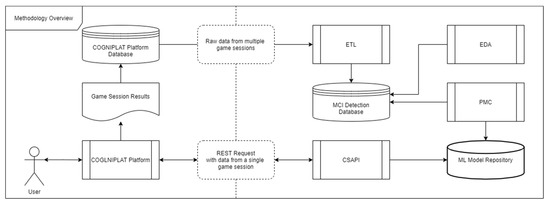
Figure 1.
Methodology overview.
3.1. COGNIPLAT Platform and Data Collection
The data used in this work were collected in the context of COGNIPLAT project (A Gaming PLATform for Restoration of COGNItive Functions of the Elderly People) [28]. A basic aim of this project is to design and implement a serious gaming platform based on rehabilitation methods suggested by the scientific research, so that its employment as part of a therapeutic program, would alleviate MCI symptoms. The COGNIPLAT game platform was built based on a multi-disciplinary approach combining theories of neuropsychology, cognitive linguistics and speech therapy organized in six domains, one diagnostic and five training domains focused on enhancing cognitive functions through different game exercises. In addition, the platform has been designed to automatically adjust the complexity and type of exercises by adapting the cognitive requirements of the games to the characteristics of each patient through an ontology-based knowledge model [29]. In this work data from ten serious games used in the diagnostic mode were collected. Table 2 describes the game types and the associated cognitive functions.

Table 2.
COGNIPLAT games used in this study and the corresponding cognitive function targeted.
Every game played earns points. Different points are awarded for each successful game at a different difficulty level. The calculation of points is based on a formula that combines the level of difficulty and the difference between the completion time of the game and the total time available. The formula for calculating the total score is given below:
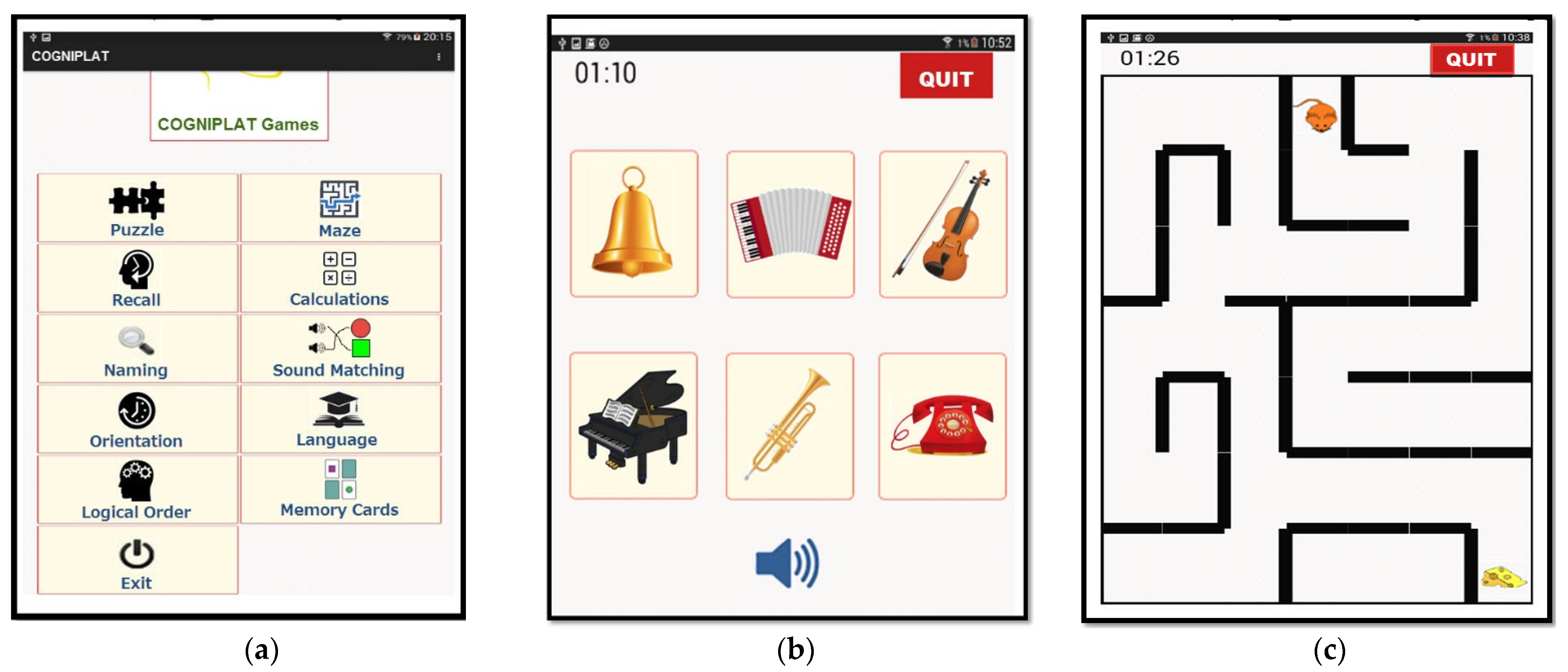
The design and development of the COGNIPLAT platform was based on the principles of user-centered design in terms of its technological dimension. In recent years there has been a shift in the creation of user-centered systems, especially in the field of health, which while providing care and support, this is done in a way that the patient is not mentally burdened, while entertainment is served. Each game screen was designed in such a way that useful conclusions can be drawn about the performance achieved, such as the speed of initial interaction with the game screen, the speed of successful completion of each task, the number of tasks successfully completed and other relevant statistics that can be collected. Figure 2 provides some examples of COGNIPLAT game screens.
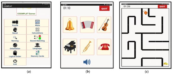
Figure 2.
Examples of COGNIPLAT game screens: (a) the main menu; (b) the sound matching game; (c) the maze game.
The most important feature of the games is the ability to statistically analyze and draw useful conclusions from them. Taking into account the history of player performance and using game performance data, it is possible to observe performance over time and any changes can be noted and analyzed. In addition, the cognitive profile and cognitive status of each user can be monitored through game analysis. The adaptability or the ability of the system to dynamically adapt the difficulty of the game to the players is an additional important feature of the platform.
An experimental evaluation study of the COGNIPLAT platform took place with the participation of 10 elderly at a daily care center (7 male and 3 female, mean 76.1 ± 7.05 years of age, mean 9.60 ± 2.37 years of education). The games were accessible as an Android application on a tablet device. Each participant had the opportunity to complete twelve game sessions during the evaluation period, which lasted for about three months. During the study, the subjects had the freedom to play any of the games for an arbitrary number of rounds and in any order.
Although the main objective of the experimental study was to assess the feasibility, engagement and acceptance of serious games for the elderly people, leveraging on this evaluation our aim is to classify participants to cognitive levels by using data which were collected from the game platform and relevant questionnaires. The MoCA test was used to assess the ground truth cognitive level of the participants and their score ranged between 20 and 28 (mean 24.40 ± 2.88). MoCA has been validated for the Greek population by providing normative data [30]. Table 3 gives the distribution of the participants according to the MoCA diagnostic classification [30] and other basic characteristics of the sample.

Table 3.
Distribution of participants according to their MoCA score and basic characteristics.
MCI participants were distinguished from the “healthy group” with a cutoff score of 23 (2 cases) for low educational level (≤6 years) and a cutoff score of 26 (4 cases) for middle educational level (7–12 years). The mean MoCA score for the MCI group was 22.50 ± 1.87 and the corresponding score for the Normal group was 27.25 ± 0.96. The morphology of the sample for the two groups has similar characteristics in terms of age and gender. The mean age is comparable between the two groups although the variance is higher in the MCI group. The mean education years of the MCI group was 8.5 ± 2.26 and for the Normal group was 11.25 ± 1.50. The technology familiarity (e.g., frequency of computing devices and internet usage) was assessed with relevant questionnaire items in a scale of 0 to 4 and was found to be less than average for the MCI group (1.83 ± 0.75) and above average for the Normal group (2.50 ± 0.58).
The MoCA test can assess various cognitive domains of a subject, such as attention, concentration, executive functions, memory, language, visuospatial, as well as abstraction, delayed recall and orientation. The assessment is administered in approximately 10 min. The total points a subject can score is 30. The person who administers the assessment, sums the subtotals of each individual task that are recorded on the right-hand of the questionnaire during the MoCA process.
On top of that, an additional questionnaire was administered in order to collect demographic, medical and lifestyle information. A classification of the questionnaire data is performed according to standardized categories [31], as shown in Table 4.

Table 4.
Grouping of questionnaire data according to the type of medical data source.
The data concerning the in-game performance of each subject is contained in two tables, the game sessions holding data such as which user is logged in and when, and the game rounds holding data such as game type, difficulty level, game outcome (success/fail), game completion time, earned points and other details regarding a single game round. During the evaluation period, in terms of recorded data entries, there were 10 subjects, 10 different game types, 119 game sessions and 2951 game rounds in total. These data are essential for this study in order to answer the main research question.
3.2. Extract-Transform-Load
The process of ETL plays a crucial part in our methodology. The main purpose that it serves is to merge all the data from the individual schemas, due to the fact that during the evaluation multiple tablet devices were used and each tablet had its own local database. The merging was done after a database migration to a new slightly improved schema.
3.2.1. Data Extraction and Partial Preprocessing
The schema migration was done in order to create parameter tables for each field with categorical values and use the key field from those parameter tables whenever these values are referenced in other tables such as game sessions and rounds. In turn, this practice helped to reduce the need for encoding functions until later in the EDA process. However, a drawback of this practice is that it can only be applied on ordinal features, since the non-ordinal features would still need to be treated with more appropriate techniques such as One-Hot-Encoding, as it was done for the feature of marital status.
3.2.2. Data Transformation and Feature Engineering
The next step, as part of the data transformation and before data loading at the scripting level, is feature engineering [32]. This process includes arithmetic and cumulative transformations to produce new features that were later inspected in the EDA process, for their importance and correlation to the target classification class.
In addition, apart from a couple of features with random values that were created to be used as reference points of the minimum importance a feature can have [33], the rest represent aggregated information about game rounds. The reason to customarily define how new features are calculated, instead of applying brute force or any other existing feature selection technique is the necessity for these features to be explainable and recreatable. The former is required to know exactly what a feature represents in a specific context, in other words to know how it relates to the target class. As for the latter, it denotes the ability to understand how the value of a feature is calculated, since this is essential to set up the process that recreates the feature from raw data of future datasets before feeding them to the model for the actual prediction.
The engineered features typically are aggregated data of individual game rounds found in a game session, as for example, total points earned in a session and average game completion time in a session. Other more composite aggregations can be also defined such as the importance of a game type which is measured as the ratio between total points won in successful game rounds of a game type in a session divided by the average points won in successful rounds for that particular game type in all sessions recorded. Table 5 gives an outline of the features that were defined and used in the MCI detection methodology.

Table 5.
The entire feature set defined and explored in the developed models.
3.2.3. Data Loading
The output of the ETL process is a data view that contains the information required to train the machine learning models. The dataset contains 119 instances with all the features derived from each game session. The last step, therefore, of the process is to load the data, at the scripting level for starting the EDA process.
3.3. Exploratory Data Analysis
The exploratory analysis could be described as the main process in the effort to create models, measure their performance and draw a conclusion regarding the research question of this work. The aim of this process is to explore all the important aspects that would provide a better understanding of the collected data and will support making decisions on the importance of each feature, testing various ML algorithms and observing the results to avoid overfitting and underfitting. Additionally, it is the most appropriate process to compare different standardization strategies, in other words secure the model from concept drift in future datasets. Python and the Scikit-learn library [34] were used as the development environment for the experimentation process.
The EDA process receives as input the data formulated at the end of the ETL process. The output of the EDA process takes the form of the information inferred by its sub-processes, which will enable the selection of the optimal feature set, the best performing algorithm and the most suitable optimizations. At this stage and before starting any data transformation, getting the quantile and the descriptive statistics of the engineered features, as shown in Table 6 and Table 7 respectively, allows one to gain a better insight of the data.

Table 6.
Quantile statistics of the game-based engineered features.

Table 7.
Descriptive statistics of the game-based engineered features.
3.3.1. Target Class Selection
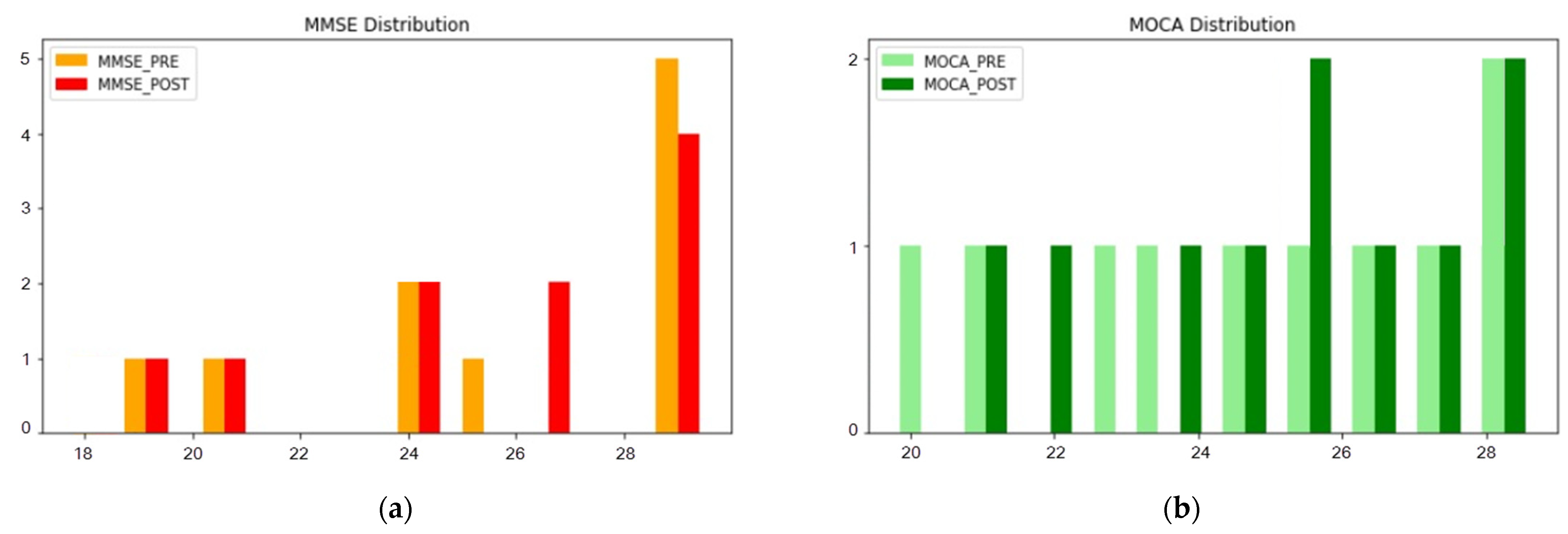
Given that the participants of the study were invited to complete both the MMSE and the MoCA cognitive assessments, before and after using the COGNIPLAT platform, there are more than one candidate variables that could be used as the target class. Aiming to select one of these two assessments, the criterion that was most influential had to do with the distribution of scores across the scale of cognitive performance for the MMSE (Figure 3a) and the MoCA (Figure 3b). Both assessments have a similar value range between 1 and 30, however, the cutoff scores of the different cognitive levels differ significantly for each assessment type. This is important as it affects the difficulty to distinguish a subject between the cognitive classes.

Figure 3.
(a) Distribution of MMSE scores before (MMSE_PRE) and after (MMSE_POST) the intervention; (b) Distribution of MoCA scores before (MOCA_PRE) and after (MOCA_POST) the intervention.
As initially demonstrated by Nasreddine [6], the ranges between the cognitive levels are much less discrete in the MMSE assessment compared to the MoCA assessment. Other researchers confirmed also that the MoCA assessment presents a much better sensitivity in distinguishing subjects with MCI compared to the MMSE due to the fact that often subjects are achieving higher scores in the latter assessment [35]. Finally, normative data for the Greek population are available for the MoCA scale but not for the MMSE.
Therefore, in this study the MoCA assessment was selected. In particular, the test performed before using the COGNIPLAT platform was chosen due to the following reasons. Firstly, because the two tests were performed in a relatively short period of time it allowed subjects to score better in the latter one due to repetition. Secondly, even with a moderate usage of serious games designed to train cognitive abilities it was expected to have a positive impact on the follow up MoCA test. Thirdly, as shown in Figure 3b, the distribution of scores in the first MoCA assessment (MOCA_PRE) was slightly more homogeneous than the distribution in the second assessment (MOCA_POST).
3.3.2. Preprocessing
Missing Values Management
In the case of our dataset, the only entries with missing values were a few entries representing game rounds that terminated due to application exceptions. Since these rounds were only a few and they had most of their fields missing the decision was to discard and not include them in the schema migration following the tuple ignoring technique [36].
Management of Outliers
Outliers apply only to values of fields that represent in-game data and not to fields that are related to the demographics and other questionnaires that the subjects completed and cannot deviate from predefined values. Given that the size of the dataset is relatively limited, removing entries that contain outlier values in one or more fields is probably not the best option. On the other hand, leaving those values as-is could potentially affect the results in the process of scaling, depending on the algorithm that will be selected to apply.
Ideally, when a game session resembles an assessment, it provides a specific number of game rounds, in a specific order, with a specific difficulty progression. The COGNIPLAT platform which was used for data gathering serves a dual goal both for cognitive assessment and for exercising cognitive functions of the elderly. As a consequence, the level of difficulty was customizable allowing the application or the caregiver to adjust it in order to meet the capabilities of each subject. On the other hand, the game performance in terms of points won in a game round is directly related to the game difficulty level. Additionally, the subjects had the option to repeat a level for several times. These characteristics resulted in some game sessions with distinctly differentiated scores.
The way the issue of outliers was addressed was by value replacement and by applying the Winsorization technique [37]. The technique was implemented to calculate new values based on the following strategy. If the feature represented a total, for example the total points gathered in the successful game rounds of a session, and the value for this feature in an entry was too high, then it was replaced with the maximum value (Q3 + 1.5*IQR) of the distribution of the feature. Respectively the low-end outlier values of an entry for a feature representing a total value, were replaced by the minimum value (Q1 + 1.5*IQR) of the distribution. On the other hand, for features that represent an average value, for example the average completion time of a successful game round, the outlier values were replaced by the median value of their distribution.
Both discretization and scaling can be affected by outliers, therefore the process that manages the outliers was explicitly placed to precede both discretization and scaling to avoid any effect of outliers in the outcome of these processes [38].
Discretization
Although discretization by binning is a relatively simple data transformation, in our methodology binning of feature values to higher levels is an essential step and it has been applied for the target class and for features derived from in-game data with continuous values.
Firstly, discretization was applied to the target class, which represents the MoCA scores recorded before the game sessions. The implementation is affected by the type of the target class field because it defines what kind of ML algorithms, between regression and classification, can be used to train the model. Additionally, this affects the way a prediction is interpreted, since an answer in the MoCA range of results would give a specific estimate while the objective is to get a broader estimate of the cognitive level of the subject as a classification between two cognition levels: normal cognition (NC) and mild cognitive impairment (MCI).
Secondly, before moving to feature selection, some normalization method needs to be applied to avoid the outweighing of features with low value ranges. In the case of the target class, the exact range of each bin is known beforehand, which happens to be the MoCA cutoff scores of each cognitive level. However, in the case of the rest of the features several binning methods are available to be applied, since discretization can be achieved with various strategies, such as equal width levels, equal frequency levels or any other custom approach. What was used on the implementation level, was the KBinsDiscretizer method of the Scikit-learn library, with the quantile option, which is described as an equal frequency discretization strategy [34].
Low Variance Features Removal
The first step that was done towards feature selection was the removal of any low to zero variance features. Those features have no useful information to offer to the model, thus, a threshold was set and in case the values of a feature are the same in 80% or more of the total entries, that feature is removed. As a result of applying this method, the features of “smoking”, “alcohol”, “hypertension” and the importance of the Calculations game were removed from the dataset. Although most of the feature selection steps follow the preprocessing, on an implementation level, the step of low variance removal precedes the data standardization to avoid having the variance threshold method being affected by the transformation of the values.
Data Standardization
Standardization has been used to further ensure that values of our features will be on the same scale and thus avoid certain features being outweighed. By applying this technique, effects from a potential concept drift in future datasets is minimized [39]. Furthermore, standardization of individual features is considered a prerequisite for many of the classifiers to be able to perform as expected [34]. The standardization method that was applied is literally an implementation of the Z-score normalization technique, where the mean of each feature distribution is centered at 0 and the values are scaled to represent the result of the division by the feature standard deviation.
3.3.3. Feature Selection
Following the data curation that was described in the preprocessing section, the methodology continues with the process that most of the data mining and ML guides define as feature selection. The advantages of reducing the features to a subset of them are well described in the literature [40], and affects many aspects of a ML experiment, such as the speed of training, the accuracy and the explainability of a model.
Feature selection algorithms, based on their output, can be categorized into two different categories. The first category is feature weighting which returns the same number of input features along with their weights by employing wrapper feature selection algorithms. The second category is subset selection which returns a subset of the input features by employing either a filter or embedded model feature selection algorithms.
Our methodology involved the selection of two feature subsets based on two different strategies. The first strategy primarily aims at creating a subset of features in which at least some of the in-game related features will be included. The mandatory inclusion of some of these features is related to the research question of this work, since it would have been pointless to train a model based only on data from the questionnaires. The second strategy used the method of feature selection with the chi2 statistic as the scorer function, a method that eliminates features with low correlation to the target class.
Feature Correlation Inspection
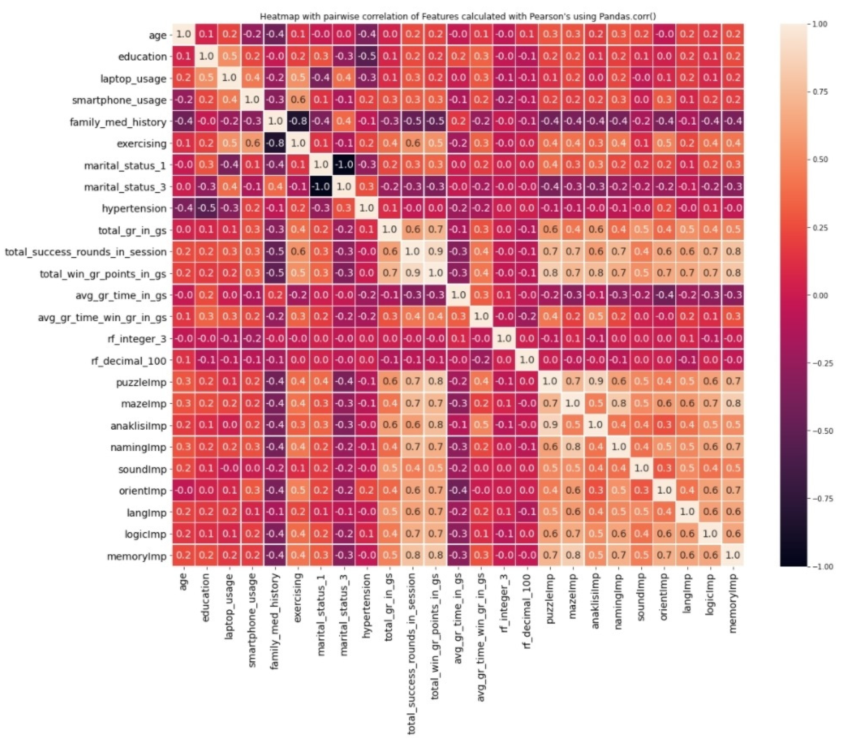
At first, the pairwise correlation between each feature is inspected. For this task, Pearson’s correlation was calculated and projected on the heatmap shown in Figure 4. The purpose at this stage is to recognize the highly correlated features and eliminate the so-called redundant features, which are those that cannot append additional information to the model [41].
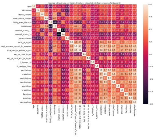
Figure 4.
Heatmap of pairwise correlation of features calculated with Pearson’s correlation.
To avoid the daunting task of manually using the heatmap to find the highly correlated features, a function that performs agglomerative clustering, was used, resulting in feature clusters separated based on the degree of their correlation which were previously calculated [42]. The dendrogram in Figure 5 projects the clusters that are formed based on a threshold value of 36% that was empirically selected and represents the maximum pairwise distance observed which in this case happens to be 4.68.
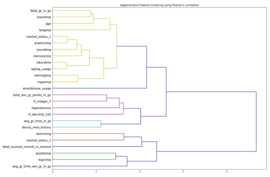
Figure 5.
Dendrogram of the feature clusters created with Pearson’s correlation values.
Feature Importance Inspection
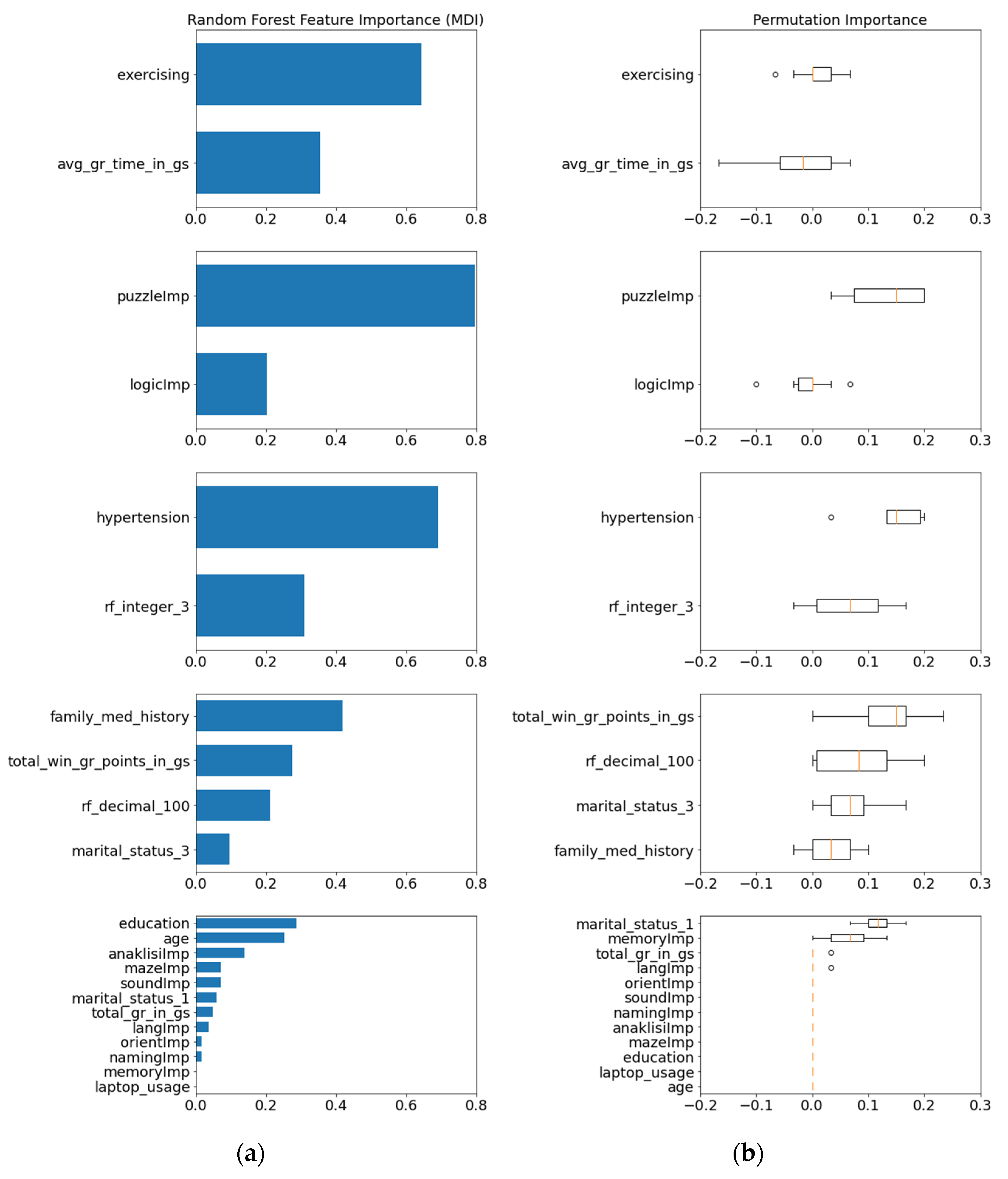
Having every feature grouped into clusters of highly correlated features, the next step of the methodology is to inspect their significance against the target class, with the ultimate goal of keeping only the most important one of each cluster. To decide whether a feature is important or not two metrics were incorporated, the mean decrease in impurity (MDI) and the mean decrease in accuracy (MDA), also known as permutation importance. Essentially, this is a form of feature weighting, thus a wrapper method is needed in order to calculate these metrics. The wrapper method that was implemented incorporates a Random Forest classifier that is used as an estimator both for the MDI and the MDA metrics. The wrapper method was then called once for the complete set of features, excluding those already removed in the preprocessing, and then once for each cluster separately (Figure 6a,b).
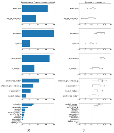
Figure 6.
(a) Results of MDI metrics for every feature cluster; (b) Results of MDA metrics for every feature cluster.
To proceed with the custom selection process, judging by the MDA and MDI scores, the features that appear to perform worse than the two randomized features were excluded, followed by the exclusion of the less important features of each cluster. The features that remained after the low variance feature removal, were inspected for their pairwise correlation and for their importance against the target class in order to create an optimized feature subset. This subset is identified next as the manually selected features.
Apart from the custom wrapper method that was implemented to measure the MDA and MDI metrics, another wrapper method that measures the P-value and the F-score for each feature, was used for an automatic selection of the k-best features. Figure 7 projects the values of these metrics for each feature cluster.
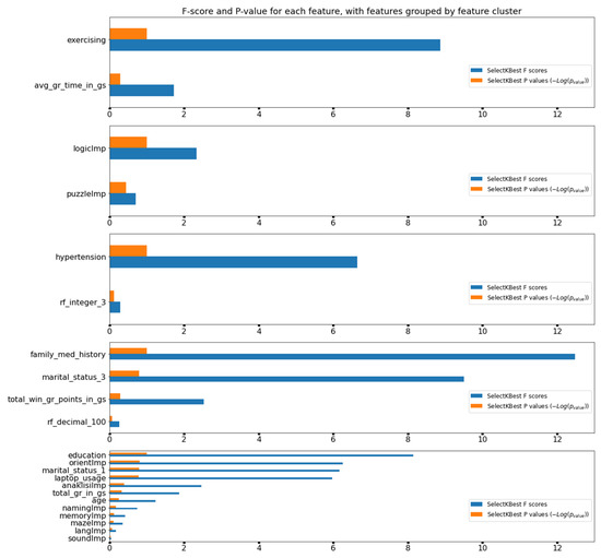
Figure 7.
Results of F-score and P-value metrics for each feature cluster.
Thus, a second subset was created using an automatic feature selection method which selects features according to the k highest scores by computing the chi2 statistic. This subset is identified next as the automatically selected features. In Table 8, the feature subsets for each feature selection strategy is provided.

Table 8.
Overview of feature subsets for each selection strategy.
3.3.4. Classifier Selection
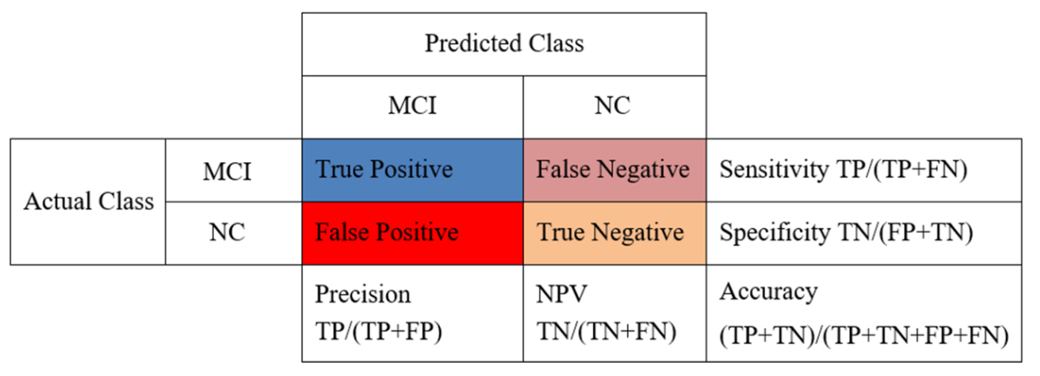
Having completed the preprocessing and the feature selection, the next major step of the EDA process for this methodology is the classifier selection. The outcome of this process is the performance evaluation of a series of ML algorithms. The criteria for whether an algorithm performs well or not, besides accuracy, is any indication about the bias and the variance of the model and also the statistics regarding the sensitivity and specificity metrics (Figure 8).
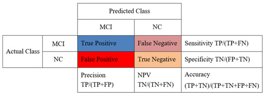
Figure 8.
Primary model evaluation metrics definition based on the mapping of the positive-negative labels between the actual and the predicted class.
As already stated, the final model would have the role of complementing screening tests like the existing MoCA and MMSE assessments, which means that it aims to be a tool to provide the likelihood, and not a definitive answer, of someone having MCI or not, as per the definitions of diagnostic and screening tests presented in the work of Trevethan [43]. Therefore, given that the outcome of our work is a binary classification model that distinguishes subjects, between having or not MCI, the most appropriate metrics to take into account for model performance evaluation appear to be those of sensitivity and specificity. This is also backed up by the plethora of publications that examine the performance of the MoCA assessment where the sensitivity and specificity metrics have been the focus of the evaluation [30,44].
From a machine learning perspective, in order for a model to continue being accurate in future datasets, the bias/variance tradeoff needs to be taken into consideration. In other words, the model needs to be accurate enough, yet able to generalize effectively, disregarding any noise in data [45].
The following ML algorithms have been tested for the aforementioned evaluation metrics: logistic regression (LR), decision tree (DT), random forest (RF), support vector classifier (SVC), k-nearest neighbors (kNN), Gaussian Naive Bayes (GNB), multi-layer perceptron (MLP) and a custom ensemble that includes all the ML algorithms except from MLP and the output of the base models is combined considering a majority voting aggregation function. At this stage, two models were trained for each type of algorithm, one for each selected feature subset (Table 8). Those models serve as baseline models and their results as a reference point to evaluate the difference in performance after performing the optimization process.
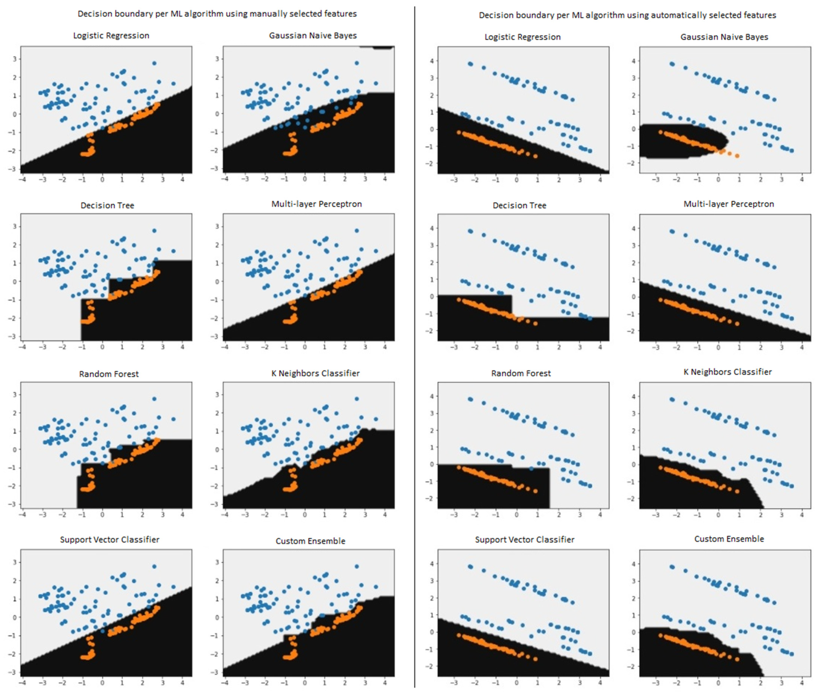
To accomplish that kind of evaluation of the models, apart from the percentage of accuracy, which is a good starting point to recognize overfitting, the decision boundary for each model has been plotted, as shown in Figure 9. The way the decision boundary helps in the process of model evaluation is by allowing the inspection of the model complexity and how it would behave with noise such as outliers in data [46].
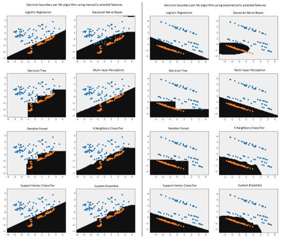
Figure 9.
Decision boundaries for each ML model for the manually (on the left) and the automatically (on the right) selected features. Each dot represents a game session entry, where the blue dots in the light background represent game sessions of subjects within the MCI class and the orange dots in the dark background represent game sessions of subjects with the NC class.
However, plotting the decision boundary on a two-dimensional plane presupposes a similar dimensionality of the dataset, otherwise we would have to repeat the plotting multiple times, each time for a features pair. The solution to that problem, on the implementation level, was given by plotting the decision boundary after applying the principal component analysis (PCA) method [47], where the dataset consists of two component features and the target class.
3.3.5. Optimization
At this stage, having trained and evaluated a series of baseline models, various optimization techniques are applied in order not only to improve the evaluation metric scores but also to improve the interpretability of these models. The optimization scenarios with the methods applied to the baseline models are outlined in Figure 10.
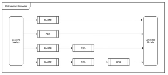
Figure 10.
Optimization scenarios that describe which methods were applied and in what order.
Data Augmentation
A major issue that had to be addressed in order to avoid biased results in our model was the imbalanced number of game sessions between the two target classes, MCI and NC. Two of the widely used methods to solve that problem are undersampling and oversampling. Since the dataset is of relatively small dimensionality, especially after the process of feature selection, undersampling would probably be a good option. However, due to the fact that the dataset also has a rather small number of entries, the oversampling method was preferred, in order to avoid discarding useful information. At the implementation level the algorithm used was the synthetic minority oversampling technique (SMOTE) [48].
Interestingly, there seems to be a discussion on whether oversampling should be applied before or after feature selection. In this work, the approach which introduces oversampling after the feature selection was preferred, in order to avoid having artificially created data affecting the feature selection process, as similarly suggested by other studies [49].
Dimensionality Reduction
The PCA technique is one of the most well-known techniques for dimensionality reduction. Although PCA is fully capable of replacing the process of feature selection, especially if the dimensionality of a dataset is not too large [50], it is incorporated in our methodology for a different reason.
The first reason is to repeat the experiment having extracted a small number of components and see if there is any fluctuation in accuracy and the rest of the metrics used to evaluate the baseline models. The second reason is to reduce the dimensionality to a number of components that would allow the dataset to be visualized along with the decision boundary of each model. This means a reduction to either two components and plotting the dataset into a two-dimensional plane with the decision boundary being a line, or three components and plotting the dataset into a three-dimensional space with the decision boundary being a plane.
As illustrated in the optimization scenarios workflow (Figure 10), PCA has been applied in two different cases, right after the baseline models and after the oversampling. For the actual implementation, the first step in utilizing PCA is to decide the optimal number of principal components to extract. This was done using the GridSearchCV method of the Scikit-learn library, which allows to inspect the accuracy of a classifier having the number of components as a variable. The Gaussian Naive Bayes was the classifier selected for that process and the range of the components was set between 1 and the number of features minus one. In addition, cross-validation was used to get a standard deviation for the accuracy for each number of components. As seen in the grid search results on Figure 11, the case with two components presents the optimal performance between 0.95 and 0.99 accuracy. For further increase in the number of components, from 3 to 6, clear evidence of overfitting is shown since the model reaches an accuracy between 0.97 and 1.
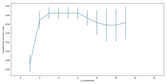
Figure 11.
Classification accuracy with SD per number of principal components, created with grid search to find the optimal number of components.
The next step in applying PCA, is to observe the results by plotting the components against the total variance that they represent, as shown in Figure 12a and also the entire dataset, after the transformation, against the target class to inspect how easily the two classes could be distinguished as shown in Figure 12b.
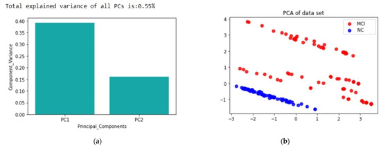
Figure 12.
(a) Percentage of variance explained per principal component; (b) Two dimensional depiction of the principal components against the target classes.
Hyperparameter Optimization
One of the most applied methods for hyperparameter optimization (HPO) is grid search. From a computational perspective, it is a costly operation since it essentially is a brute force black-box task. However, it allows us to find the optimal values for the parameters of multiple algorithms without human interaction. According to the literature, one can find a few alternatives to grid search, such as the population-based methods of random search, genetic algorithms, particle swarm optimization, the Bayesian optimization methods and others that are less computationally expensive [51]. However, for this work, since the dataset is of relatively small size, the grid search method was preferred.
3.4. Production Model Creation
To be able to claim that one of the trained models can be considered production ready, the aforementioned optimization processes are not sufficient. There is at least one important factor that could potentially introduce bias to the trained models and that is data leakage, as it is well described by Bussola et al. [52]. The final process of this methodology focuses on solving that issue.
Amongst all the possible forms data leakage can take, we focus on solving the leakage that could possibly occur during preprocessing from the training subset to the testing subset. The culprit, for this type of data leakage, is considered to be the transformations that the dataset goes through during the preprocessing and more specifically the transformations that precede the splitting of the dataset between training and testing subsets [53].
The challenge that arises here is the fact that we are already at a late stage regarding the methodology workflow, considering that even optimization has already been applied. Thus, to be able to implement a solution for data leakage, we incorporated a method to safely preprocess and train a model after splitting the dataset. On the other hand, a major advantage of this practice is that upon prediction there is no need to separately load any transformers to edit the future data, instead, preprocessing is now part of the model itself.
3.5. Classification Service API
For the final stage of the proposed methodology, we have experimented with building a classification service Application Programming Interface (API) to study and record any challenges that could come up from such a task. The structure of this service is rather simple, as it consists of a Flask server with a main method that loads the model and a controller to receive REST requests for prediction from the COGNIPLAT game suite application. In a production environment, these requests would contain the in-game data recorded throughout a game session. The response returned from the controller contains the label of the cognitive class predicted by the loaded model, i.e., MCI or NC and the confidence score for the specific prediction, given of course that the loaded model supports the export of that information.
4. Results
To evaluate the trained models, a wrapper function was created to efficiently get the metric scores, relevant confusion matrices and the receiver operating characteristic (ROC) with the area under curve (AUC) and the precision–recall diagrams. The evaluation of each classification model is performed by applying the k-fold (k = 5) cross validation technique on a stratified hold-out sub-dataset that was kept initially specifically for the purpose of model evaluation. A split of the initial dataset was performed yielding a training sub-dataset (70% of the dataset) and a test sub-dataset (30% of the dataset). The performance of models with different configurations is then evaluated on the hold-out set, for the purpose of selecting the best performing model. This approach is useful to measure the prediction performance of the final production model or compare predictions with reference to held-out samples [54].
The performance results of all the models trained are presented in two separate tables. Table 9 records the results that are related to the baseline models, the application of the SMOTE, PCA and HPO methods using the two feature subsets selected. Table 10 records the results of the models that were trained using pipelines. A pipeline in the context of ML can be described as a utility method that allows the design of a procedure from the data preprocessing to the training of the classifier offering some advantages over the manual execution of these steps. The purpose of the pipeline is to assemble the above methods that can be cross-validated together while setting different parameters in the context of using the Scikit-learn library [55]. The pipeline method eventually implements the solution for avoiding data leakage.

Table 9.
Evaluation results, by ML algorithm, for the training and testing processes, for both feature selection strategies, from the stage of baseline models up to applying hyperparameter optimization.

Table 10.
Evaluation results, by ML algorithm, for the training and testing processes, for both feature selection strategies using the pipeline method.
In Table 9, the accuracy of each model is provided both for the training and the testing dataset. In the latter case the cross-validation accuracy is shown. At this point, by inspecting the accuracy during training and testing it is possible to recognize which algorithms tend to create models that overfit or underfit. Therefore, first a set of baseline models are trained and tested, then SMOTE and PCA are applied separately, followed by the application of combined SMOTE and PCA on the same dataset and finally a set of models are created by combining SMOTE, PCA and hyperparameter optimization. By inspecting the results, it is observed that most of the baseline trained models for the manually selected features tend to either overfit or underfit, contrary to the dataset composed of the automatically selected features. Moving to the results of the datasets when the SMOTE technique is applied, a slight decrease of overfitting for the dataset of the manually selected features and a significant increase of overfitting for the dataset with the automatically selected features are observed. Inspecting the datasets when the PCA method is applied, a significant underfitting for both datasets can be observed. Examining the results after the sequential application of both SMOTE and PCA, a better consistency of the accuracy for both datasets is observed ranging between 85.14% and 95.56% for the dataset with the manually selected features and between 89.78% and 97.78% for the dataset with the automatically selected features. Finally, only marginal variations in performance are observed when comparing these results to those that are achieved from the sequential application of SMOTE, PCA and HPO for the dataset with the manually selected features and in some cases for the dataset with the automatically selected features where the models either present overfitting (SVC, MLP) or underfitting (custom ensemble).
Moving on to the results of the next stage of our methodology, the final models of this study are given which are built with the usage of pipelines to avoid any possible bias from data leakage. For these models, there is an interest to study their performance in terms of sensitivity and specificity as shown in Table 10. The first conclusion that can be drawn from this evaluation is that for both datasets there are models that score 100% on accuracy in training, so these models clearly overfit and they should be discarded. Hopefully, there are also models that do not overfit during the training, yet they do maintain relatively acceptable scores regarding the accuracy and the rest of the evaluation metrics. Taking into account the scores of sensitivity and specificity, we can distinguish as the best performing models those that are trained using the SVC and GNB algorithms. More specifically, the SVC based model yields an accuracy of 91.79% (6.74% SD), a sensitivity of 93.20% (6.33% SD) and a specificity of 90% (10% SD) for the dataset trained on the manually selected features, while the GNB based model yields an accuracy of 92.14% (8.2% SD), a sensitivity of 93.4% (6.2% SD) and a specificity of 90% (10% SD) for the dataset trained on the automatically selected features. Another remark about this batch of models is the relatively abrupt values of the specificity metric, which is related to the fact that the SMOTE is now part of the pipeline, thus the oversampling for the minority class happens much later than the dataset split, which consequently leads small numbers in false positives to have significant impact on specificity.
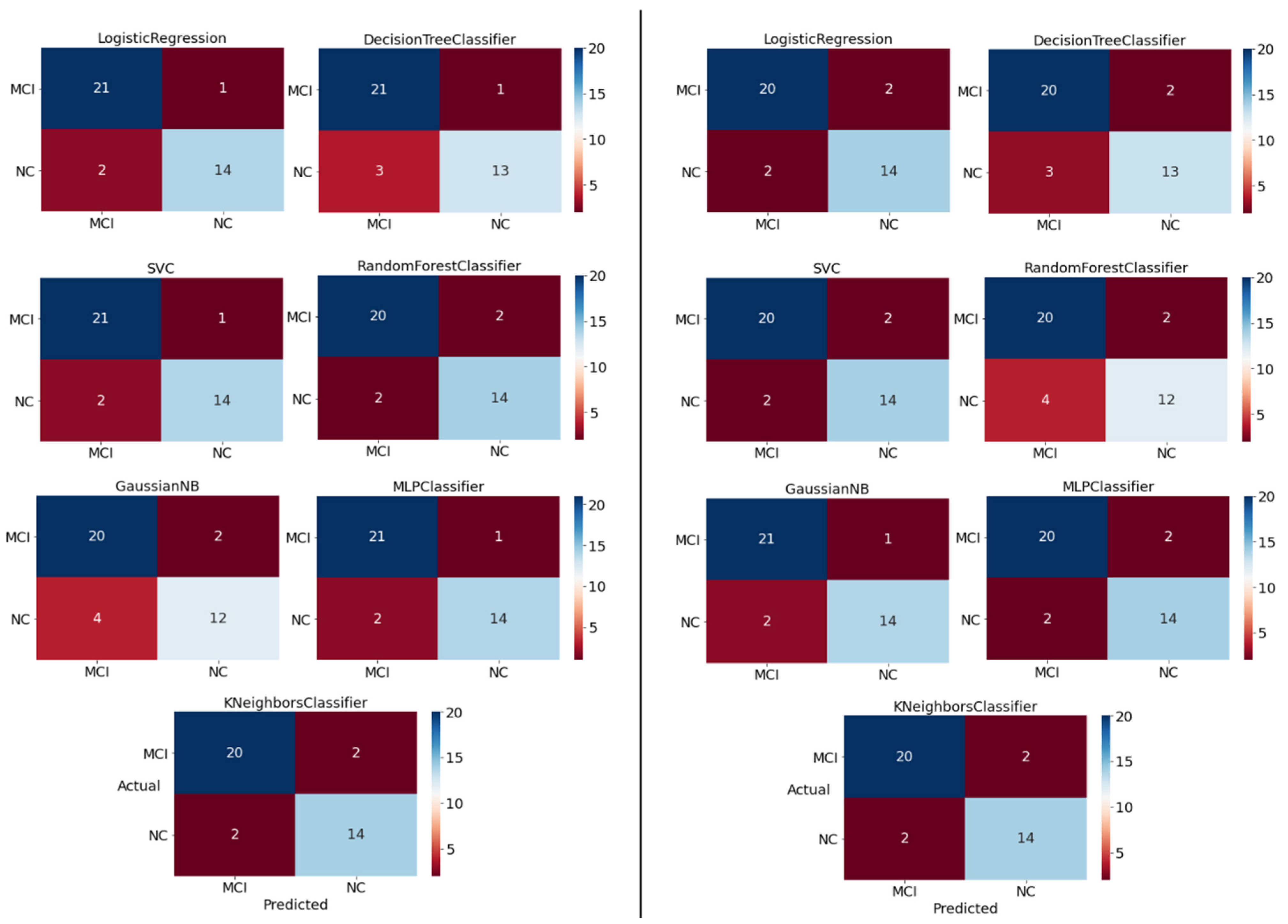
Figure 13 provides relevant confusion matrices to visualize the classification performance of the models using the testing dataset for a single prediction. Note that the testing dataset is a stratified hold-out sub-dataset, roughly 30% of the original dataset, yielding 38 instances.

Figure 13.
Confusion matrix per ML algorithm for the models trained using the pipeline method for the manually selected features (on the left) and the automatically selected features (on the right).
The custom wrapper method for model evaluation is also configured to plot the ROC-AUC and the precision–recall diagrams as shown in Figure 14 and Figure 15, respectively. The AUC of SVC for the production level model and the manually selected features is 0.98 whereas the AUC of GNB for the automatically selected features is 0.97. These diagrams along with the precision–recall diagrams affirm the efficiency of the aforementioned ML models.
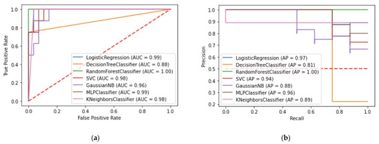
Figure 14.
(a) ROC-AUC for the production level models and the manually selected features; (b) Precision–recall/sensitivity for the production level models and the manually selected features.
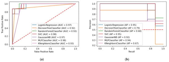
Figure 15.
(a) ROC-AUC for the production level models and the automatically selected features; (b) Precision–recall/sensitivity for the production level models and the automatically selected features.
5. Discussion
This work has shown that it is possible to create ML models based on data collected from serious games and transformed to engineered features along with relevant subjective information. These models can be used then to accurately classify whether a subject belongs to the MCI or NC group as attested by the MoCA cognitive test. In this context, a focal point of the research performed was the development of a custom methodology to train such MCI detection models with low bias and variance and to validate the models using established and solid metrics and techniques, while being attentive to maintain high performance in terms of sensitivity and specificity.
There are 31 features that originally were defined to train the models from which 15 are related to the games, 14 are related to demographic and health data and 2 are artificial variables used as reference points to filter features with a lower importance than them during the feature selection process. Mixing technology-based and subjective data in order to improve the predictive performance of a cognitive impairment detection model is not unprecedented, as a similar approach has been demonstrated in other studies [56]. The inclusion of features that represent demographics, health and lifestyle cater for improving not only the performance but also the generality of the prediction. As a matter of fact, such factors are taken into account also when traditional assessments are used to evaluate cognitive impairment [57]. For example, in MoCA assessment, a score adjustment is allowed depending on the education level of the subjects [6,30].
For the production model trained with the manually selected features and the Support Vector Classifier integrating all the optimization techniques and in the context of the pipeline method an accuracy of 91.79%, a sensitivity of 93.20% and a specificity of 90% were achieved. On the other hand, for the production model trained with the more verbose set of automatically selected features using the Gaussian Naive Bayes algorithm under the pipeline context, the corresponding evaluation metrics were 92.14%, 93.4% and 90%. However, for the specificity metric a higher standard deviation is observed which is due to the fact that for the creation of the production model the testing dataset does not undergo the oversampling process which is now part of the pipeline and happens later in the workflow. Consequently, the true negative values are fewer and therefore small errors of the model lead to a large variation. Both feature selection strategies lead to models with roughly equal performance however the model with the manually selected features is 18% more compact. This model includes 9 features with 5 of them representing game data and 4 of them representing subjective data.
The COGNIPLAT game suite includes games which target cognitive functions that are linked to the assessment of MCI. From the features that have been selected in the machine learning models it is observed that the games that are associated with the cognitive areas of short-term memory, visual memory, episodic memory, spatio-temporal orientation and executive functions are the most important predictors of cognitive impairments. This is reasonable since the design of the corresponding games focused on several occasions on porting typical cognitive assessments in a gamified environment. For example, the Orientation game was inspired by Weschler’s Picture Arrangement Subset [58] which is used to assess perception and problem-solving cognitive operations that are associated with spatio-temporal orientation. The Logical Order game is a digital emulation of the Wisconsin Card Sorting Test [59], frequently used to assess executive functions. The Recall game is a gamified version of the Digit Span Forward Test, a subsection also of the MoCA test, typically used to assess short-term memory. The Naming game is a gamified version of the Rey Auditory Verbal Learning Test [60] where the auditory stimuli are replaced by visual probes to assess the episodic memory. Consequently, this design approach ensures that each gameplay assesses the cognitive operation that was meant for.
The use of ML algorithms for cognitive impairment identification on the basis of game and subjective data goes beyond the classical approach of using statistical techniques. The MCI detection problem, as defined, calls for employing supervised ML algorithms for classification. Several such ML algorithms were evaluated in order to build the most effective models including probabilistic classifiers (i.e., LR and GNB), kNN, SVC, decision tree learning (i.e., DT, RF), neural networks (i.e., MLP) and ensemble learning. These algorithms were selected based on their suitability regarding the characteristics of the problem in hand and from a research perspective they provided the opportunity to test the created dataset on a broad spectrum of different methods for classification. The choice of ML algorithms is in accordance with other studies, especially in the area of disease prediction in the healthcare domain [61]. The best classification models for MCI detection that the proposed methodology delivered were based on SVC (an implementation of the support vector machine method in the Scikit-learn library) and GNB which are ranked amongst the top ML algorithms with superior accuracy in related problems [61]. The SVC algorithm proved capable of efficiently handling the mixed feature scope (in-game and subjective data) and showed endurance in the overfitting risk. On the other hand, GNB is a well-known classifier which is simple and able to handle both discrete and continuous data achieving a high performance even when the training dataset is limited.
There are several challenges that must be addressed in order to build an MCI detection model using data collected from serious games. Starting with the data available for model training an important issue had to do with their unequal distribution between the two categories of the target class. In particular, the game sessions that correspond to subjects in the MCI category were 71, in contrast to those in the NC category, which were 48. This issue could lead to the creation of biased models with respect to the majority class. To address this, the oversampling method was applied using the SMOTE algorithm, as described in the optimization task of the EDA process. Another data issue is related to features with very low variance which had almost the same values for all the subjects. These features were excluded from the model training (such as the alcohol and smoking variables) within the low variance feature removal procedure. Finally, due to the relatively small dataset, there is a limit to the application of more complex machine learning algorithms, such as deep learning algorithms.
Data leakage is another important issue to resolve. The effects of data leakage are essentially the possible alteration of performance results as the testing data are involved in the process of creating (fitting) the model. The solution to this problem was to use the pipeline utility method, where all transformations of the EDA stage are performed in a closed process that contains no elements of the testing dataset. The advantages of the pipeline include the encapsulation of the data transformations and the classifier, the ability to be used along with grid-search and the prevention of data leakage given that a dataset is split between training and testing sub-datasets beforehand. In our work, the usage of pipelines, apart from the data-leakage prevention and the overall simplicity in workflow design, offers the convenience of having the data preprocessing transformations included in the final model itself, which is very important for the deployment of the classification Service API. This allows new data to be loaded in a single entry point to get a prediction.
One of the optimization techniques applied was dimensionality reduction. In particular, the PCA technique was applied, thus managing to transform the independent variables of the dataset (i.e., the features) into two principal components, which contained a percentage of the original variance. There are other dimensionality reduction techniques that could be used. One alternative method is the linear discriminant analysis (LDA), which in contrast to the PCA method is a supervised learning technique, taking into account the target class for the creation of new components. The difficulty of the LDA method is that the number of new components that emerge is specific and is always the lowest value between the number of features and the number of categories of the target class. In our case this means that only one component could be used.
A limitation of the present study is that the number of participants is apparently small to draw safe conclusions even though the design of the study and the assembled sample were meticulously handled in terms of methodology (e.g., sample heterogeneity, informed consent, ethical approval). Undoubtedly, a larger sample would provide a sounder base regarding the effectiveness of the methodology. On the other hand, the dataset for training and testing the classification models consists of 119 instances, which correspond to the number of game sessions played by the participants. Each instance contains up to 32 variables, i.e., 31 features (as presented in Table 5) and 1 binary classification state. This configuration plausibly serves our preliminary study aiming to assess whether serious games combined with machine learning methods could potentially work as a tool for cognitive screening.
The research described in this paper could be enhanced in various directions. An extension of the research approach will be to explore a model that can classify multiple classes such as NC, MCI and Dementia given the diagnostic capability of the MoCA assessment. Since many subcategories of MCI have been identified such as amnestic MCI, single domain MCI, multiple domain MCI, dysnomic MCI, dysexecutive MCI and their combinations [62], it would be challenging to examine the association of low performance in specific games with specific MCI subcategories in order to create a model that would be able to classify multiple cognitive classes.
6. Conclusions
This work demonstrates that models trained on data gathered from serious games can distinguish, with sufficient accuracy, whether an individual belongs in the healthy or the MCI state in terms of cognitive competency. The research performed in this work is multifaceted and its scope ranges from the healthcare application domain in terms of exploring MCI characteristics, to the use of serious games in terms of collecting raw data and to the machine learning domain in terms of extracting features and building models that allow the early MCI detection. The contribution of this work is a methodology to train and evaluate models with ML algorithms, validate their results and reflect on the challenges addressed throughout the steps of this process. Eventually, the ultimate goal is to use the games and the machine learning models in services that could be used supplementary to the traditional cognitive assessment tools. Our preliminary results are promising and call for further research in the way to bring this methodology to the clinical practice of cognitive impairment diagnosis.
Author Contributions
C.G. planned and supervised the study, and C.K. designed the ML methodology. Analyses and writing of the manuscript were performed by both C.G. and C.K. Both authors have read and agreed to the published version of the manuscript.
Funding
This research has been co-financed by the European Regional Development Fund of the European Union and Greek national funds through the Operational Program Competitiveness, Entrepreneurship and Innovation, under the call ERA-NETS 2018 (ID:Τ8ΕΡA2-00011, grant MIS:5041669).
Institutional Review Board Statement
The study was conducted according to the guidelines of the Declaration of Helsinki and approved by the Institutional Review Board (or Ethics Committee) of University of the Aegean.
Informed Consent Statement
Informed consent was obtained from all subjects involved in the study.
Data Availability Statement
The datasets generated during and/or analyzed during the current study are not publicly available due to ethical constraints in consideration of participants’ privacy but are available from the corresponding author on reasonable request.
Acknowledgments
The authors would like to thank Georgios Koumanakos, Dimitrios Koumanakos and Maria Frounta from Frontida Zois for their support in implementing the evaluation study and the volunteers that took part in the study.
Conflicts of Interest
The authors declare no conflict of interest.
References
- Plassman, B.L.; Williams, J.W., Jr.; Burke, J.R.; Holsinger, T.; Benjamin, S. Systematic review: Factors associated with risk for and possible prevention of cognitive decline in later life. Ann. Intern. Med. 2010, 153, 182–193. [Google Scholar] [CrossRef] [PubMed]
- Langa, K.M.; Levine, D.A. The diagnosis and management of mild cognitive impairment: A clinical review. JAMA 2014, 312, 2551–2561. [Google Scholar] [CrossRef]
- Albert, M.S.; DeKosky, S.T.; Dickson, D.; Dubois, B.; Feldman, H.H.; Fox, N.C.; Gamst, A.; Holtzman, D.M.; Jagust, W.J.; Petersen, R.C.; et al. The diagnosis of mild cognitive impairment due to Alzheimer’s disease: Recommendations from the National Institute on Aging-Alzheimer’s Association workgroups on diagnostic guidelines for Alzheimer’s disease. Alzheimer’s Dement. 2011, 7, 270–279. [Google Scholar] [CrossRef]
- Petersen, R.C. Mild cognitive impairment as a diagnostic entity. J. Intern. Med. 2004, 256, 183–194. [Google Scholar] [CrossRef]
- Folstein, M.F.; Robins, L.N.; Helzer, J.E. The mini-mental state examination. Arch. Gen. Psychiatry 1983, 40, 812. [Google Scholar] [CrossRef]
- Nasreddine, Z.S.; Phillips, N.A.; Bédirian, V.; Charbonneau, S.; Whitehead, V.; Collin, I.; Cummings, J.L.; Chertkow, H. The Montreal Cognitive Assessment, MoCA: A brief screening tool for mild cognitive impairment. J. Am. Geriatr. Soc. 2005, 53, 695–699. [Google Scholar] [CrossRef] [PubMed]
- Tong, T.; Chignell, M.; Tierney, M.C.; Lee, J. A serious game for clinical assessment of cognitive status: Validation study. JMIR Serious Games 2016, 27, e5006. [Google Scholar] [CrossRef] [PubMed]
- Krishnan, K.; Rossetti, H.; Hynan, L.S.; Carter, K.; Falkowski, J.; Lacritz, L.; Cullum, C.M.; Weiner, M. Changes in Montreal Cognitive Assessment scores over time. Assessment 2017, 24, 772–777. [Google Scholar] [CrossRef] [PubMed]
- Valladares-Rodriguez, S.; Fernández-Iglesias, M.J.; Anido-Rifón, L.; Facal, D.; Rivas-Costa, C.; Pérez-Rodríguez, R. Touchscreen games to detect cognitive impairment in senior adults. A user-interaction pilot study. Int. J. Med. Inform. 2019, 127, 52–62. [Google Scholar] [CrossRef]
- Jin, R.; Pilozzi, A.; Huang, X. Current Cognition Tests, Potential Virtual Reality Applications, and Serious Games in Cognitive Assessment and Non-Pharmacological Therapy for Neurocognitive Disorders. J. Clin. Med. 2020, 9, 3287. [Google Scholar] [CrossRef]
- Sawyer, B. Serious Games: Improving Public Policy through Game-Based Learning and Simulation; Woodrow Wilson International Center for Scholars: Washington, DC, USA, 2002. [Google Scholar]
- Boletsis, C.; McCallum, S. Smartkuber: A serious game for cognitive health screening of elderly players. Games Health J. 2016, 5, 241–251. [Google Scholar] [CrossRef]
- Ge, S.; Zhu, Z.; Wu, B.; McConnell, E.S. Technology-based cognitive training and rehabilitation interventions for individuals with mild cognitive impairment: A systematic review. BMC Geriatr. 2018, 18, 213. [Google Scholar] [CrossRef] [PubMed]
- Lumsden, J.; Edwards, E.A.; Lawrence, N.S.; Coyle, D.; Munafò, M.R. Gamification of cognitive assessment and cognitive training: A systematic review of applications and efficacy. JMIR Serious Games 2016, 4, e5888. [Google Scholar] [CrossRef]
- McCallum, S.; Boletsis, C. Dementia games: A literature review of dementia-related serious games. In International Conference on Serious Games Development and Applications; Springer: Berlin/Heidelberg, Germany, 2013; pp. 15–27. [Google Scholar]
- Garcia-Ceja, E.; Riegler, M.; Nordgreen, T.; Jakobsen, P.; Oedegaard, K.J.; Tørresen, J. Mental health monitoring with multimodal sensing and machine learning: A survey. Pervasive Mob. Comput. 2018, 51, 1–26. [Google Scholar] [CrossRef]
- Valladares-Rodríguez, S.; Pérez-Rodríguez, R.; Anido-Rifón, L.; Fernández-Iglesias, M. Trends on the application of serious games to neuropsychological evaluation: A scoping review. J. Biomed. Inform. 2016, 64, 296–319. [Google Scholar] [CrossRef]
- Joshi, V.; Wallace, B.; Shaddy, A.; Knoefel, F.; Goubran, R.; Lord, C. Metrics to monitor performance of patients with mild cognitive impairment using computer based games. In Proceedings of the 2016 IEEE-EMBS International Conference on Biomedical and Health Informatics (BHI), Las Vegas, NV, USA, 24–27 February 2016; pp. 521–524. [Google Scholar]
- Leduc-McNiven, K.; White, B.; Zheng, H.; McLeod, R.D.; Friesen, M.R. Serious games to assess mild cognitive impairment: ‘The game is the assessment’. Res. Rev. Insights 2018, 2. [Google Scholar] [CrossRef]
- Leduc-McNiven, K.; Dion, R.T.; Mukhi, S.N.; McLeod, R.D.; Friesen, M.R. Machine learning and serious games: Opportunities and requirements for detection of mild cognitive impairment. J. Med. Artif. Intell. 2018, 2. [Google Scholar] [CrossRef]
- Solana, J.; Cáceres, C.; García-Molina, A.; Chausa, P.; Opisso, E.; Roig-Rovira, T.; Menasalvas, E.; Tormos-Muñoz, J.M.; Gómez, E.J. Intelligent Therapy Assistant (ITA) for cognitive rehabilitation in patients with acquired brain injury. BMC Med. Inform. Decis. Mak. 2014, 14, 58. [Google Scholar] [CrossRef]
- Banerjee, S.; Chattopadhyay, T.; Biswas, S.; Banerjee, R.; Choudhury, A.D.; Pal, A.; Garain, U. Towards wide learning: Experiments in healthcare. arXiv 2016, arXiv:1612.05730. [Google Scholar]
- Sirály, E.; Szabó, Á.; Szita, B.; Kovács, V.; Fodor, Z.; Marosi, C.; Salacz, P.; Hidasi, Z.; Maros, V.; Hanák, P.; et al. Monitoring the early signs of cognitive decline in elderly by computer games: An MRI study. PLoS ONE 2015, 10, e0117918. [Google Scholar]
- Binaco, R.; Calzaretto, N.; Epifano, J.; McGuire, S.; Umer, M.; Emrani, S.; Wasserman, V.; Libon, D.J.; Polikar, R. Machine learning analysis of digital clock drawing test performance for differential classification of mild cognitive impairment subtypes versus Alzheimer’s disease. J. Int. Neuropsychol. Soc. 2020, 26, 690–700. [Google Scholar] [CrossRef]
- Valladares-Rodriguez, S.; Pérez-Rodriguez, R.; Fernandez-Iglesias, J.M.; Anido-Rifón, L.E.; Facal, D.; Rivas-Costa, C. Learning to detect cognitive impairment through digital games and machine learning techniques. Methods Inf. Med. 2018, 57, 197–207. [Google Scholar] [CrossRef]
- Schröer, C.; Kruse, F.; Gómez, J.M. A Systematic Literature Review on Applying CRISP-DM Process Model. Procedia Comput. Sci. 2021, 181, 526–534. [Google Scholar] [CrossRef]
- Martínez-Plumed, F.; Contreras-Ochando, L.; Ferri, C.; Orallo, J.H.; Kull, M.; Lachiche, N.; Quintana, M.J.; Flach, P.A. CRISP-DM twenty years later: From data mining processes to data science trajectories. IEEE Trans. Knowl. Data Eng. 2019, 33, 3048–3061. [Google Scholar] [CrossRef]
- COGNIPLAT Project. Available online: https://cogniplat.aegean.gr/ (accessed on 27 July 2021).
- Goumopoulos, C.; Igoumenakis, I. An Ontology based Game Platform for Mild Cognitive Impairment Rehabilitation. In Proceedings of the ICT4AWE, Online Streaming, 21–27 June 2020; pp. 130–141. [Google Scholar]
- Poptsi, E.; Moraitou, D.; Eleftheriou, M.; Kounti-Zafeiropoulou, F.; Papasozomenou, C.; Agogiatou, C.; Bakoglidou, E.; Batsila, G.; Liapi, D.; Markou, N.; et al. Normative data for the Montreal Cognitive Assessment in Greek older adults with subjective cognitive decline, mild cognitive impairment and dementia. J. Geriatr. Psychiatry Neurol. 2019, 32, 265–274. [Google Scholar] [CrossRef]
- Weber, G.M.; Mandl, K.D.; Kohane, I.S. Finding the missing link for big biomedical data. JAMA 2014, 311, 2479–2480. [Google Scholar] [CrossRef] [PubMed]
- Nargesian, F.; Samulowitz, H.; Khurana, U.; Khalil, E.B.; Turaga, D.S. Learning Feature Engineering for Classification. In Proceedings of the Twenty-Sixth International Joint Conference on Artificial Intelligence (IJCAI-17), Melbourne, Australia, 19–25 August 2017; pp. 2529–2535. [Google Scholar]
- Stoppiglia, H.; Dreyfus, G.; Dubois, R.; Oussar, Y. Ranking a random feature for variable and feature selection. J. Mach. Learn. Res. 2003, 3, 1399–1414. [Google Scholar]
- Pedregosa, F.; Varoquaux, G.; Gramfort, A.; Michel, V.; Thirion, B.; Grisel, O.; Blondel, M.; Prettenhofer, P.; Weiss, R.; Dubourg, V.; et al. Scikit-learn: Machine learning in Python. J. Mach. Learn. Res. 2011, 12, 2825–2830. [Google Scholar]
- Aggarwal, A.; Kean, E. Comparison of the Folstein Mini Mental State Examination (MMSE) to the Montreal Cognitive Assessment (MoCA) as a cognitive screening tool in an inpatient rehabilitation setting. Neurosci. Med. 2010, 1, 39. [Google Scholar] [CrossRef]
- Han, J.; Pei, J.; Kamber, M. Data Mining: Concepts and Techniques; Elsevier: Amsterdam, The Netherlands, 2011. [Google Scholar]
- Ghosh, D.; Vogt, A. Outliers: An evaluation of methodologies. In Proceedings of the 2012 InJoint Statistical Meetings, San Diego, CA, USA, 28 July–2 August 2012; Volume 2012. [Google Scholar]
- Brownlee, J. Data preparation for machine learning: Data cleaning, feature selection, and data transforms in Python. In Machine Learning Mastery; Machine Learning Mastery Pty. Ltd.: Vermont, VIC, Australia, 2020. [Google Scholar]
- Sobolewski, P.; Wozniak, M. Concept Drift Detection and Model Selection with Simulated Recurrence and Ensembles of Statistical Detectors. J. Univers. Comput. Sci. 2013, 19, 462–483. [Google Scholar]
- Liu, H.; Motoda, H.; Setiono, R.; Zhao, Z. Feature selection: An ever evolving frontier in data mining. In Proceedings of the Feature Selection in Data Mining, PMLR, Hyderabad, India, 21 June 2010; pp. 4–13. [Google Scholar]
- Koller, D.; Sahami, M. Toward Optimal Feature Selection; Stanford InfoLab: Stanford, CA, USA, 1996. [Google Scholar]
- Müllner, D. Modern hierarchical, agglomerative clustering algorithms. arXiv 2011, arXiv:1109.2378. [Google Scholar]
- Trevethan, R. Sensitivity, specificity, and predictive values: Foundations, pliabilities, and pitfalls in research and practice. Front. Public Health 2017, 5, 307. [Google Scholar] [CrossRef] [PubMed]
- Goldstein, F.C.; Ashley, A.V.; Miller, E.; Alexeeva, O.; Zanders, L.; King, V. Validity of the montreal cognitive assessment as a screen for mild cognitive impairment and dementia in African Americans. J. Geriatr. Psychiatry Neurol. 2014, 27, 199–203. [Google Scholar] [CrossRef]
- Briscoe, E.; Feldman, J. Conceptual complexity and the bias/variance tradeoff. Cognition 2011, 118, 2–16. [Google Scholar] [CrossRef] [PubMed]
- Lever, J.; Krzywinski, M.; Altman, N. Points of significance: Model selection and overfitting. Nat. Methods 2016, 13, 703–705. [Google Scholar] [CrossRef]
- Wall, M.E.; Rechtsteiner, A.; Rocha, L.M. Singular value decomposition and principal component analysis. In A Practical Approach to Microarray Data Analysis; Springer: Boston, MA, USA, 2003; pp. 91–109. [Google Scholar]
- Blagus, R.; Lusa, L. SMOTE for high-dimensional class-imbalanced data. In BMC Bioinform; Rok, B., Lara, L., Eds.; BioMed Central: London, UK, 2013; Volume 14, p. 106. [Google Scholar]
- Tang, L.; Liu, H. Bias analysis in text classification for highly skewed data. In Proceedings of the Fifth IEEE International Conference on Data Mining (ICDM’05), Houston, TX, USA, 27–30 November 2005; p. 4. [Google Scholar]
- Kosmpoulos, A.; Paliouras, G.; Androutsopoulos, I. The effect of dimensionality reduction on large scale hierarchical classification. In International Conference of the Cross-Language Evaluation Forum for European Languages; Springer: Berlin/Heidelberg, Germany, 2014; pp. 160–171. [Google Scholar]
- Feurer, M.; Hutter, F. Hyperparameter optimization. In Automated Machine Learning; Springer: Berlin/Heidelberg, Germany, 2019; pp. 3–33. [Google Scholar]
- Bussola, N.; Marcolini, A.; Maggio, V.; Jurman, G.; Furlanello, C. AI Slipping on Tiles: Data Leakage in Digital Pathology. In Pattern Recognition. ICPR International Workshops and Challenges; Springer: Berlin/Heidelberg, Germany, 2021; pp. 167–182. [Google Scholar]
- Saravanan, N.; Sathish, G.; Balajee, J.M. Data wrangling and data leakage in machine learning for healthcare. Int. J. Emerg. Technol. Innov. Res. 2018, 5, 553–557. [Google Scholar]
- Chen, P.H.; Liu, Y.; Peng, L. How to develop machine learning models for healthcare. Nat. Mater. 2019, 18, 410–414. [Google Scholar] [CrossRef] [PubMed]
- Assunção, F.; Lourenço, N.; Ribeiro, B.; Machado, P. Evolution of scikit-learn pipelines with dynamic structured grammatical evolution. arXiv 2020, arXiv:2004.00307. [Google Scholar]
- Alhanai, T.; Au, R.; Glass, J. Spoken language biomarkers for detecting cognitive impairment. In Proceedings of the 2017 IEEE Automatic Speech Recognition and Understanding Workshop (ASRU), Okinawa, Japan, 16–20 December 2017; pp. 409–416. [Google Scholar]
- Milani, S.A.; Marsiske, M.; Cottler, L.B.; Chen, X.; Striley, C.W. Optimal cutoffs for the Montreal Cognitive Assessment vary by race and ethnicity. Alzheimer’s Dement. Diagn. Assess. Dis. Monit. 2018, 10, 773–781. [Google Scholar] [CrossRef]
- Wechsler, D. Wechsler Adult Intelligence Scale, 3rd ed.; Harcourt Assessment: San Antonio, TX, USA, 1997. [Google Scholar]
- Heaton, R.K.; Chelune, G.J.; Talley, J.L.; Kay, G.G.; Curtiss, G. Wisconsin Card Sorting Test (WCST): Manual: Revised and Expanded; Psychological Assessment Resources: Lutz, FL, USA, 1993. [Google Scholar]
- Schmidt, M. Rey Auditory Verbal Learning Test: A Handbook; Western Psychological Services: Los Angeles, CA, USA, 1996. [Google Scholar]
- Uddin, S.; Khan, A.; Hossain, M.E.; Moni, M.A. Comparing different supervised machine learning algorithms for disease prediction. BMC Med. Inform. Decis. Mak. 2019, 19, 281. [Google Scholar] [CrossRef]
- Díaz-Mardomingo, M.D.; García-Herranz, S.; Rodríguez-Fernández, R.; Venero, C.; Peraita, H. Problems in classifying mild cognitive impairment (MCI): One or multiple syndromes? Brain Sci. 2017, 7, 111. [Google Scholar] [CrossRef] [PubMed]
Publisher’s Note: MDPI stays neutral with regard to jurisdictional claims in published maps and institutional affiliations. |
© 2021 by the authors. Licensee MDPI, Basel, Switzerland. This article is an open access article distributed under the terms and conditions of the Creative Commons Attribution (CC BY) license (https://creativecommons.org/licenses/by/4.0/).


