Predicting Hard Disk Failure by Means of Automatized Labeling and Machine Learning Approach

Abstract

Today, cloud systems provide many key services to development and production environments; reliable storage services are crucial for a multitude of applications ranging from commercial manufacturing, distribution and sales up to scientific research, which is often at the forefront of computing resource demands. In large-scale computer centers, the storage system requires particular attention and investment; usually, a large number of diverse storage devices need to be deployed in order to match the varying performance and volume requirements of changing user applications. As of today, magnetic drives still play a dominant role in terms of deployed storage volume and of service outages due to device failure. In this paper, we study methods to facilitate automated proactive disk replacement. We propose a method to identify disks with media failures in a production environment and describe an application of supervised machine learning to predict disk failures. In particular, a proper stage to automatically label (healthy/at-risk) the disks during the training and validation stage is presented along with tuning strategy to optimize the hyperparameters of the associated machine learning classifier. The approach is trained and validated against a large set of 65,000 hard drives in the CERN computer center, and the achieved results are discussed.

1. Introduction

The new frontiers of industrial production and scientific research are reflected in a growing demand for computing and, consequently, in an evolution of storage technologies. The increased demand for data storage and processing pushes the data-centers to provide increasingly efficient services [1]. This efficiency requirement can be compromised by the devices that underpin storage: hard drives. Magnetic hard disks are currently among the most widely used and devices for storing data.

Magnetic hard disks are currently among the most widely used and among the most frequently failing components of storage systems and disk failures, resulting in about 78% of cloud server system failures [2].

In addition to the impact of a service outage for the user, these events also result in significant costs for the service provider. As unscheduled interventions, they may require rapid (and hence costly) human intervention or a resource intensive consistency check and re-validation of recent processing steps by a combination of the service provider and user. In the worst case, disk failures can lead to permanent data loss and hence economical damage to the user and service provider due to a breach of service level agreements [2,3,4]. While fault tolerance techniques can reduce the risk of loss, they also often impact negatively on system performance or price per usable volume.

In order to facilitate the automated interpretation of the disk operational status, the disk vendors introduced Self-Monitoring, Analysis and Reporting technology (SMART), a standardized monitoring system with the goal to warn about an increasing likelihood of disk failures. The SMART subsystem is a firmware component running on the disk processor and continuously collects operational metrics in order to generate a warning or error messages before disk failures that affect the integrity of application data.

The characteristics of SMART technology include a number of attributes for diagnostics, the SMART attribute implementation technology varies from model to model, even for different disk models of the same manufacturer [5].

The goal of the SMART system is to warn a user at least 24 h before device failure [6]. Each manufacturing company implements SMART sensors according to their proprietary technology choices and sets alarm thresholds with the aim of an acceptable rate of false-alarms and its potential impact on drive warranty obligations. Generally, the false-alarm rate is around 0.1% per year [7,8].

Several methods based on modeling techniques have been proposed to recognize hard drives that need to be replaced using SMART attributes [8,9,10,11], but none of them meet all the needs of adapting to heterogeneous sets of hard drives, low false positive and false negative rates, automatic preliminary dataset labeling.

To overcome the limitations considered before, we propose an inference method to retrieve information about failed disks and a supervised machine learning approach to build a predictor of near-failure disks. The method presented in this paper does not need a human intervention for dataset labeling and is capable of operating with heterogeneous sets of magnetic hard disks.

The proposal has been validated in a case study at the European Organization for Nuclear Research (CERN), where the High Energy Physics (HEP) challenges have led storage services to become a crucial part of the cloud services [12].

CERN uses a variety of models [13], and an effective prediction of a likely drive malfunction would allow increasing the user’s perceived service quality and, at the same time, decrease the resources to operate the service.

The remainder of this paper is organized as follows: in Section 2, we set the scene with a brief review of the state-of-the-art technology in hard disk failure prediction; in Section 3, we provide a short summary of the machine learning algorithm we have chosen, followed, in Section 4, by a detailed description of its application to our classification problem. In the conclusion, we summarize the results obtained by applying our method to the CERN disk population (Section 5) and outline future extensions of our approach.

2. Prediction in Hard Disk Replacement

An automated and standardized hard disk replacement process can be defined based on the results from automatic testing framework, which is integrated by disk manufacturers in their disk firmware: the SMART system. The hard disk models used in storage centers are often numerous and change over time. Due to the heterogeneity of hard disks of which datacenters are often composed, it is not possible to perform analytical modeling. So modeling by means of machine learning is the best solution in this context. Multiple recent approaches based on SMART attributes have been proposed and show improved prediction performance in general but are usually highly dependent on the specific device they were applied to.

A Gaussian Mixture based the fault detection approach has been proposed in 2017, which is able to minimize the False Alarm Rate (FAR) of 0%, but its performance drops by a few dozen percentage points in the hours before the last 24 h, and there is no information on the rate of false alarms in the days before the last. In addition, the method has been tested on a single hard disk model [8].

The authors of [10] propose a technique based on Online Random Forests. Their method reaches an accuracy (defined as the fraction of true positives and true negatives in the whole population) above 93% while maintaining a low rate of false positives (i.e., failure predicted for an actually healthy disk). To achieve this result, this technique considers hard disk metrics over the period of one week. It predicts a disk failure in case any of the smart metrics in the period is positive and is hence sensitive to transient phenomena. Good results have been reached using an offline machine learning technique based on a decision forest named Regularized Greedy Forest (RGF) [14]. Only two cases of hard disk models were explored for which a recall (defined as the fraction of correctly detected failures among all positives) value as high as approximately 98% was achieved. The corresponding results for the false positives rate are not mentioned explicitly but can be derived as approximately 2% [14].

An interesting approach based on the Long Short Term Memory model has been proposed in [15] that achieves good results in terms of the false alarms rate. This paper does not present a labeling method for broken disks; thus, it is not clear how to create the dataset for the machine learning models. Moreover, it does not introduce a solution on how to deal with heterogeneous sets of hard drive models.

The authors of [11] focus on the wide-spread heterogeneity of data-centers. They addressed the issue of the manufacturer dependencies of the implementation technology, which the SMART monitoring system is integrated with. The authors compare Decision Trees, Neural Networks and Logistic Regression and suggest Decision Tree as the best solution for the problem at hand. The method proposed is able to predict about 52% of all hard disk failures among the truly failed drives.

3. Regularized Greedy Forest Model

The Regularized Greedy Forest model proposed in [16] is a variant of a Gradient Boosted Decision Tree with an explicit regularization (introduced with a regularization term in the loss function) and with a repeated full-correction of the coefficients (a repeated optimization). The RGF model and the algorithm for its training are briefly described to clarify the steps that follow in the paper. The RGF is a forest, or more formally, a non-linear function class $h:X⟶\{0,1\}$, where X is a set of input vector $\mathit{x}=[x\left[1\right],x\left[2\right],\dots ,x\left[d\right]]\in {\mathbb{R}}^d$. The vector $y\in \{0,1\}$ is a response vector used for the supervised learning. Each node is a non-linear decision rule $\nu$ associated with the pair $({\beta }_{\nu },{\alpha }_{\nu })$. Here, ${\beta }_{\nu }$ refers to a basis function and ${\alpha }_{\nu }$ to the weight assigned to the internal node $\nu$. The model of the forest is

$$h_{\mathit{F}}\left(\mathit{x}\right)=\sum _{\nu \in \mathit{F}}{\alpha }_{\nu }{\beta }_{\nu }\left(\mathit{x}\right),$$

(1)

where ${\alpha }_{\nu }=0$ for any internal node. This forest model is accompanied with a loss function $L\left(h\right(x);y)$ and a regularization term $R\left(h\right)$. The RGF goal is to find a non-linear function $\widehat{h}\left(\mathit{x}\right)$ from a function class $\mathit{H}$ that minimizes the following risk function: $\widehat{h}=argmi{n}_{h\in H}[L(h\left(x\right),y)+R\left(h\right)]$.

The algorithm greedily selects the basis functions and optimizes the weights. The two structural operations managing the forest are (1) the splitting of nodes and (2) the introduction of additional trees. At the k-th iteration, the algorithm, in modifying the structure, operates one of the two options in order to reduce the regularized loss functions defined as: $Q\left(\mathit{F}\right)=L(h_{\mathit{F}}\left(X\right),Y)+R\left(h_{\mathit{F}}\right)$.

The addition of a new node, from which to start a new tree, consists of the sum of the node pair to the existing tree, formally: $h_{{\mathit{F}}_k}\left(\mathit{x}\right)=h_{{\mathit{F}}_{k-1}}\left(\mathit{x}\right)+\alpha \beta \left(\mathit{x}\right)$. The splitting of a node consists of the removal of the node that must be divided and the addition of the two new nodes. Assuming a generic node associated with $(\beta ,\alpha )$, $(\beta ,\alpha )$ needs to be split into $({\beta }_1,{\alpha }_1)$ and $({\beta }_2,{\alpha }_2)$ because it is the node split that minimize the loss function, the forest h at the iteration k becomes: $h_{{\mathit{F}}_k}\left(\mathit{x}\right)=h_{{\mathit{F}}_{k-1}}\left(\mathit{x}\right)-\alpha \beta \left(\mathit{x}\right)+{\alpha }_1{\beta }_1\left(\mathit{x}\right)+{\alpha }_2{\beta }_2\left(\mathit{x}\right)$. After a series of changes in the structure, the algorithm proceeds to an optimization of the weights. The algorithm then fixes the structure and adjusts the weights by evaluating all possible combinations in order to minimize the loss function. Carrying out a frequent optimization of the weights affects the calculation times.

To make RGF work with success, several parameters involved in the model training have to be suitably tuned. Three different versions of the Loss Function $L(h_{\mathit{F}}\left(X\right),Y)$ can be exploited: the Square Loss $LS:={(f\left(x\right)-y)}^2/2$, the Exponential Loss $Expo:=e^{\left(yf\right(x\left)\right)}$ or the logistic loss $Log:=log(1+e^{\left(yf\right(x\left)\right)})$ function. The regularization term $R\left(h_{\mathit{F}}\right)$ can assume three different models. In all of the three cases, the coefficient $\lambda$ weighs the importance for regularization. The first regularizer is the $L_2$ Regularization on Leaf-only Models defined as $R\left(h_T\right)=\lambda ·{\sum }_{\nu \in \mathit{T}}{\alpha }_{\nu }^2/2$. The second regularizer is the Minimum-Penalty Regularizer defined as $R\left(h_T\right)=\lambda ·\{{\sum }_{\nu \in \mathit{T}}{\gamma }^{d_{\nu }}{\beta }_{\nu }^2/2:h_{T\left(\beta \right)}\left(\mathit{x}\right)\equiv h_T\left(\mathit{x}\right)$}. The third regularizer is similar to the second, but the condition changes: the sum of the sibling pair need to be zero. The third regularizer is the Minimum-Penalty Regularizer with Sum-to-zero Sibling Constraints; the regularizer is $R\left(h_T\right)=\lambda ·\{{\sum }_{\nu \in \mathit{T}}{\gamma }^{d_{\nu }}{\beta }_{\nu }^2/2:h_{T\left(\beta \right)}\left(\mathit{x}\right)\equiv h_T\left(\mathit{x}\right);\forall \nu \notin L_T·[{\sum }_{p\left(\omega \right)=\nu }{\beta }_{\omega }=0]\}$ [16].

4. Proposed Approach

The novel method presented here is for inferencing failed hard disks (Algorithm 1) and to predict when a drive needs to be replaced due to impending failure (Algorithm 2).

From the collected data, a first step (Figure 1) of knowledge extraction is made to label the disks that have been replaced due to a failure and distinguish them from all other disks (replaced or not). After that, a cleaning of the inconsistent data is carried out, then, hyperparameters tuning, training and testing phases of an RGF model are performed consequently (Figure 2).

4.1. Automatized Labeling Stage

4.1.1. Labeling Training Data

In many environments, including the CERN storage deployment, a precise definition or label for “failed” disks is not a priori available but needs be derived from other existing information. At CERN, we have put in place a probe that several times per day determines the presence of all disk drives (identified by their serial numbers) in all server or compute nodes. Changes between these configuration snapshots are used to track interventions by the data center operations team, which usually take place for one of the following reasons: A disk is

• removed/disabled after repeated I/O or self-test errors;
• retired/replaced at the end of its planned lifetime;
• relocated within the data center(s) (e.g., due to floorspace reorganization).

In Figure 3, the hard disk $d_2$ is an example of temporary suspension during the interval $I_{\mathrm{g}}=[g_1;g_2]$. A typical scenario of a host decommissioning is also shown in the Figure 3. All drives belonging to a host that has to be shut down are drained and removed. Due to the high disk reliability, it is quite unlikely that more than one disk would fail at the same day on the same host. Thus, whenever multiple shutdowns are observed (e.g., $d_1,d_2,d_3,d_4$) in a small day interval, it is necessary not to classify these disks as replaced disks due to a failure.

As there is no available label classifying a disk as broken, we propose a heuristic approach based on the following definition for “disks at risk”, which is aimed to identify disk replacements due to individual device failures from the larger amount of disk replacements due to other data center operations (e.g., host or disk model replacements or retirement campaigns).

Definition 1.

A disk is classified as broken if it has been removed and all other hard disk belonging to the same host machine continue to operate nominally.

In other words, replaced hard disks are classified as broken if and only if neither if other HDDs are removed in the same day nor if the host machine is decommissioned within 30 days (e.g., $d_k$ at $t_k$ instant in Figure 3).

4.1.2. SMART Data

The number of hard disks required to perform good training must be reasonably large. Hard drives fail even after several years from their installation, which leads to a small number of failures per year in a storage system. To obtain sufficient SMART tuples (a complete set of SMART measures defining the health status of a disk) to train and test the proposed machine learning method, some tens of replaced hard disks have to be taken into account; this way, the SMART tuples of all hard disks must be necessarily collected in a database daily. The collected data must be accessible in order to be evaluated in their temporal sequence, and each SMART attribute tuple must be associated with the serial number, model, host machine and timestamp of the drive. The job that collects and stores this information must be run daily.

4.1.3. Pre-Processing

To suitably train the proposed method, all incorrect measures associated with errors, missing values, exceeding values, etc., must be preliminarily removed. The collected measurements may be corrupted as errors caused by the probe, in the internal network, in the file system, etc., may occur. Another typical example of a corrupt measurement can be an out-of-range temperature measurement, which can happen because the temperature sensor of a hard disk broke, but this has not affected the correct functioning of the storage device. Moreover, a disk can be turned off for several days before being switched on again. Disks disappeared from the list of monitored devices and belonging to multiple removals (due to maintenance, dismantling of hosts machine or similar) have to be excluded from the set labeled as broken units. In addition, entire measures may be missing in some days because of software errors, busy firmware, database problems, etc.

An example of the considered conditions are schematically presented in Figure 3; in particular, the hard disk $d_2$ (more specifically, its SMART tuples) are not present during a time interval, a gap.

Let us define S as the whole dataset of available hard disks in the storage system, and let $I_{\mathrm{g}}:=[g_1;g_2]$, with $g_2>g_1+1$ be a generic days gap experienced during SMART tuples acquisitions. This way, the subset $S_r\in I_{\mathrm{g}}$ of hard disks replaced during the gap has to be removed from the dataset because no assumptions can be made about their possible failure and the classification rule for broken disks is not applicable; a specific hard disk is dropped from the list of monitored devices since its host machine has been completely removed, and hard disks possibly operating have also been dismissed. On the other hand, disks normally running after the gaps are kept in the dataset. Disks replaced during an interval $S_{r,k}\in I_{\mathrm{g}+\mathrm{k}}:=[g_2;g_2+k]$ need to be excluded as well because a replacement ${\widehat{S}}_{r,k}$ that happened in the interval $I_{\mathrm{g}+\mathrm{k}}$ does not have the k days of measures needed for a consistent train dataset. Thus, the dataset becomes $S_d=S-\{S_r\in I_{\mathrm{g}},I_{\mathrm{g}+\mathrm{k}}\}$.

Afterward, a classification needs to be performed on the dataset according to Definition 1. The system must be able to recognize and process the typical measures of the last K useful days before disk replacement. To this aim, a preliminary analysis has to be carried out to understand how many days before the replacement, the SMART measures of a disk, typically, begin to significantly change.

4.2. RGF-Based Machine Learning Approach

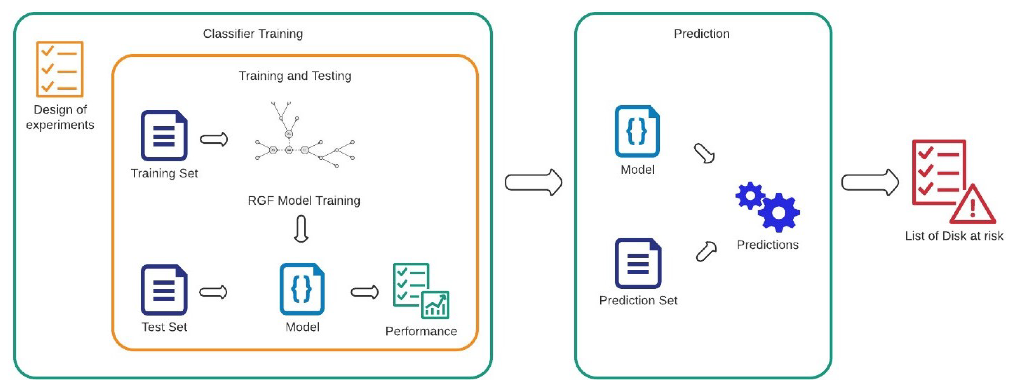
4.2.1. Training of Models

The considered dataset $S_d$ needs to be split into training, $S_L$, and test, $S_T$, sets. As there is a need to classify each hard disk according to its state of health, a binary classification distinguishing between “at-risk” $s_b$ and “not at risk” $s_h$ disks must be performed. The classification phase is performed by using the RGF model. The training algorithm requires a tuning of the hyperparameters.

The goal is to learn a single nonlinear function $h\left(\mathit{x}\right)$ on some input vectors $\mathit{x}\in S_L$ with labels Y, minimizing the argument of a loss function $L\left(h\right(X),Y)$. The algorithms used for learning can be RGF with $L_2$ regularization on leaf-only models (referred to as “RGF” in the following), or the RGF with Minimum-Penalty Regularization (“RGF_Opt”) or RGF with min-penalty regularization with Sum-to-zero Sibling constraints (“RGF_Sib”).

The number of leaves is a data-dependent hyperparameter, and its tuning affects the training time. The number of leaves can be chosen in the range of (1000, 10,000). The degree of regularization $\lambda$ can be adjusted choosing a value as small as needed $\{1,...{10}^{-20}\}$. A lower value of $\lambda$ reduces the importance of the regularization in the regularized loss functions. The hyperparameter mazimum depth $\gamma$ is a parameter used only with the two Minimum-Penalty Regularization models and indirectly tunes the importance of nodes because a smaller value ensures a lesser penalty for deeper nodes. In the two min-penalty regularizers, the $d_{\nu }$ represents the distance from the root of the generic node $\nu$, and the constant hyperparameter is elevated as ${\gamma }^{d_{\nu }}$. Thus, higher values of $\gamma$ penalizes deeper nodes. The last hyperparameter of interest is the Test Interval, i.e., the number of leaves added per each iteration. Besides the ones just listed, there are others hyperparameters whose configurations, if not defined, do not prevent model training but can help improving its efficiency and effectiveness. Their contribution will not be discussed in this paper, and the amplitudes exploited during the performance assessment have been set to their default value.

The hyperparameter tuning, together with the choice of the number of observation days, create a number of possible configurations that can rapidly reach a few thousands. A drastic reduction of the experiments number without losing significance can be made by means of a Design Of Experiments (DOE) using the Taguchi Orthogonal Array Designs [17]; in particular, each combination of factor levels exploited to carry out a specific experiment is referred to as plan configuration. Some of the considered parameters, such as the width of the observation window, lambda, the number of leaves, etc., can assume values within large intervals. The purpose of the design of experiments is to evaluate the effect of all parameters in some significant configurations for training purposes; this way, for each parameter, a suitable, limited number of values has been established according to both their typical interval of variation and authors’ knowledge and experience.

The choice of levels for each factor is limited to the number of configurations of the experiment plan used. The risk of overfitting is averted. Due to the limited number of possible combinations, it is necessary to execute the experiment plan within intervals that reasonably already give good performance. The optimal configuration is therefore identified between levels of factors that do not cause overfitting. It is also possible to make a comparison between the performances obtained in the optimal case and in all cases foreseen by the experiment plan. This further comparison allows the system to obtain the certainty of having achieved the best performance among all the tested combinations.

Usually, the goal is generally to minimize false negatives to avoid risk targets being incorrectly predicted, thus assuring a conservative behavior from an operating point of view. The accuracy index is often used in contexts of methodologies based on predictors to give a quantization of the goodness of the model. Accuracy is defined as

$$Accuracy=\frac{TruePositives+TrueNegatives}{TotalPopulation},$$

(2)

where True Positives and True Negatives are the number of disks well predicted as healthy or non-healthy, respectively. Vice-versa, the number or disk wrongly predicted are False Positives (in case of an healthy disk predicted as to be replaced) and False Negatives (for disks that need to be replaced and actually predicted as healthy). The accuracy is usually used to have a first feeling on the effectiveness of the predictor since it returns the fraction of correctly predicted test cases out of the totality of all test cases. Although this index shows correctly executed predictions, it does not measure the predictor’s sensitivity to the distinctions between positive and negative cases. The method proposed in this work uses Recall, False Positive Rate (FPR) and Positive Likelihood Ratio (LR+) to better evaluate the predictor’s performance.

The Recall index, defined as

$$Recall=\frac{TruePositives}{TruePositive+FalseNegatives}$$

(3)

is often preferred in this context; the higher the recall value, the better the reduction of false negatives.

As regards data-centers storage systems, characterized by tens of thousands of hard disks, a single percentage point of false positives corresponds, instead, to several hundred hard disks wrongly classified as “to be replaced” even if they are not. This way, in the considered application field, minimizing the false positive occurrences turns out to be as fundamental as maximizing the recall. The index associated with the risk of false positives is the False Positive Rate defined as:    

$$FPR=\frac{FalsePositives}{FalsePositive+TrueNegatives}.$$

(4)

The Taguchi DOE approach can be exploited to assess the factors’ impact on one performance index; to this aim, the Positive Likelihood Ratio ($LR+$), defined as

$$LR+=\frac{Recall}{FPR}$$

(5)

and capable of simultaneously taking into account Recall and FPR, has been exploited. Before carrying out the training stage of the RGF model, input data have to suitably shuffled in order to guarantee independence from the temporal distribution of the measures and prevent biases related to the dataset $S_d$. Both training and test experiments are required for each of the plan configurations; to this aim, the whole dataset $S_d$ is split according to a ratio of 70–30%, for training and testing, respectively.

Algorithm 1 Classifier Training.

1: procedureDataSetCollection(D) 2:     for each disk $d_i\in D$ do 3:         $S⟵$ Get SMART tuples daily of $d_i$ 4:     end for 5:     Return S 6: end procedure 7: procedurePre-processing(S) 8:     for each SMART tuple $S_i\in S$ do 9:         if $S_i$ is corrupted OR missed OR out-of-range then 10:            Remove $S_i$ from S 11:         end if 12:         Label($S_i$) according to Definition 1 13:         if $S_i$ is replaced in $[g_1;g_2+k]$ then 14:            Remove $S_i$ from S 15:         end if 16:     end for 17:     Return S 18: end procedure 19: procedureDesign of Experiment(S) 20:     T= TaguchiDesign($L_9$, replicates = 30) 21:     for each design $t_i\in T$ do 22:         $Shuffle\left(S\right)$ 23:         $S_L,S_T=Split(S,70-30\%)$ 24:         $Model=RgfTrain(t_i,S_L)$ 25:         $LR+=RgfTest(Model,S_T)$ 26:     end for 27:     Select configuration C using $EffectPlot(T,LR+)$ 28:     Return C 29: end procedure 30: procedureThreshold assessment($S,C$) 31:     $Shuffle\left(S\right)$ 32:     $S_L,S_T=Split\left(S\right)$ 33:     Get Definitive Model $Model=RgfTrain(C,S_L)$ 34:     Get Probabilities $P=RgfTest(Model,S_T)$ 35:     $RC⟵RocCurve(P,S_T)$ 36:     Select Threshold $T_c$ using $RC$ 37:     Return $T_c,Model$ 38: end procedure

The Regularized Greedy Forest is trained using the the training data set $S_{\mathrm{L}}$ and tested using the testing data set $S_{\mathrm{T}}$.

Authors suggest at least 30 runs for each plan configuration in order to simultaneously assure statistical significance and feasible execution times. For each plan configuration, the values of Accuracy, Recall and FPR, expressed in percentage terms, are calculated as the median of the Accuracy, Recall and FPR achieved in the various runs. The final index of LP+ is calculated as the ratio of the median Recall and FPR.

The RGF classifier returns a probability for each tuple of SMART measures of likelihood with respect to the two classes of healthy or broken. The last step for the user is the choice of a proper threshold beyond which discriminating whether the considered tuple identifies a Hard Disk that needs to be replaced or not. The choice of the optimal threshold turns out to be a trade-off between false and true positive rates. To drive the choice of the right threshold, the Receiver Operating Characteristic (ROC) curve has been exploited. The ROC curve, a graphic tool for the evaluation of FPR and TPR, helps the developer, in fact, to identify the best trade-off threshold, which the authors experienced close to the beginning of the curve knee.

4.2.2. Validation

The system configured and trained according to the above method can be put into production. It is useful to perform a further final validation and evaluate the trend of the probability with which each hard disk is classified as healthy or not.

Algorithm 2 Prediction.

1: procedurePrediction($T_c,D,Model$) 2:     for each disk $d_i\in D$ do 3:         $D_p$⟵ Get SMART tuples of $d_i$ 4:         $Prediction=RgfPrediction(D_p,Model,T_c)$ 5:         Return $(D_p,Prediction)$ 6:     end for 7:     Return the list of disks at risk with probabilities 8: end procedure

The tuples of SMART attributes collected daily are processed by the trained and tested RGF model. By reporting the evolution of probabilities versus time on a plot, samples corresponding to a change of the operating condition (from healthy to broken) can be identified a few days before the replacement of the hard disk.

5. Experimental Results

The proposed method has been validated on a case study at CERN; CERN has a computer center where a large volume of data generated by the complex accelerator system and experiments are stored and processed. The collected data are stored in a set of Magnetic, Solid State or Tape Hard Disks through a distributed file systems service called EOS and internally developed. There are currently roughly 65,000 magnetic drives, including 89 different models. Approximately 15,000 disk replacements occur annually due to different reasons; replacements due to bankruptcies are roughly a dozen per week. Data collected from August 2018 and October 2020 have been used for the case study experiments in Section 5.1. A remaining fraction of data collected in the months between November 2020 and January 2021 were reserved for validation in Section 5.2. An example of the algorithm implemented in R is available as supplementary material “R-Scripts” in order to encourage the reproducibility of the method.

5.1. Case Study

For the case study, the five models among those used at the CERN Data Center were examined. Selected models are those characterized by the higher cardinality in the CERN Data Center; this is a key issue since a large number of hard drives are necessary to grant a sufficient amount of information on broken disks to train the RGF model. The examined datasets are shown in

Table 1. The composition of the dataset.

Model	Healthy	Broken	Total
Ischia	11,962	81	12,043
Capri	11,238	160	11,398
Ventotene	9172	18	9190
Procida	7948	20	7968
Ponza	4695	378	5073

; it is worth noting that all considered datasets are unbalanced in terms of healthy versus replaced hard disks in favor of the healthy ones. For the sake of privacy, the vendors and models of the examined Hard Disks have been replaced with names of some Tyrrhenian islands.

Before collecting the data to train and test the RGF model, a study on the temporal distribution of the SMART measures has been carried out; as stated above, reasons why there may be gaps between the measures are manifold. Since the proposed method requires that for RGF training, tuples of hard disks classified according to Definition 1 are necessary, establishing after how many days of absence a hard disk can be considered as permanently replaced and its missing measures that are not attributable to transient conditions is a fundamental step. To this aim, the duration of gaps between the tuples greater than 1 day have been collected and organized as a histogram. The corresponding results are reported in Figure 4, where it can be noticed that the maximum number of occurrences is associated with a 5-day gap. On the contrary, the number of occurrences for gaps longer than 20 days rapidly decreases.

We decided on a conservative approach and chose to remove all the measures of the 30 days prior to the last available from the dataset. The measures of the last 30 days have however been used for the purpose of labeling hard drives. In particular, the SMART attributes considered to provide measure tuples are reported in

Table 2. Selected SMART Attributes [18].

SMART	Attribute Name	Description
01	Read Error Rate	Hardware read errors that occurred when reading data from a disk surface
03	Spin-Up Time	Average time of spindle spin up
04	Start/Stop Count	Number of spindle start/stop cycles
05	Reallocated Sectors Count	Quantity of remapped sectors
07	Seek Error Rate	Frequency of errors while positioning
09	Power-On Hours	Number of hours elapsed in the power-on state
10	Spin Retry Count	Number of retry attempts to spin up
12	Device Power Cycle Count	Number of power-on events
192	Power-off Retract Count	Number of power-off or emergency retract cycles
193	Load/Unload Cycle	Number of cycles into landing zone position
194	HDA temperature	Temperature of a hard disk assembly
197	Current Pending Sector Count	Number of unstable sectors (waiting for remapping)
198	Offline Uncorrectable Sector Count	Number of uncorrected errors
199	UltraDMA CRC Error Count	Number of CRC errors during UDMA mode

.

After extrapolating only the data relating to the hard disks shown in Table 1 from the entire dataset S, the dataset $S_d$ has been pre-processed to clean from corrupt, incomplete and error data according to what was stated in Section 4.1.3.

Once the dataset was cleaned, each hard disk’s serial (the drive’s unique identifier) was classified and labeled according to Definition 1; successively, the labeled dataset has been divided into train, $S_l$, and test, $S_t$, datasets. The training set of SMART measures of healthy disks has been randomly decimated in such a way as to assure the same cardinality of the broken drives for each disk model.

A Resolution III plan $L_9$ has been exploited for all five hard drive models, whose plan configurations are reported in

Table 3. The design of the experiment.

Experiment	Algorithm	Loss Function	Leaf	Days
1	RGF	LS	1000	6
2	RGF	Expo	5000	7
3	RGF	Log	10,000	8
4	RGF_Sib	LS	5000	8
5	RGF_Sib	Expo	10,000	6
6	RGF_Sib	Log	1000	7
7	RGF_Opt	LS	10,000	7
8	RGF_Opt	Expo	1000	8
9	RGF_Opt	Log	5000	6

.

Each configuration is characterized by at least one parameter level different from one another, thus assuring a complete and efficient investigation of the whole experimental space.

The main output of the Taguchi approach is the so-called effects diagram, i.e., the evolution of the performance index versus each parameter level; the effects diagram allows the developer to determine which level of each factor corresponds to a maximization (or minimization) of the chosen performance index. For the considered method, the goal is the maximization the $LR+$ index. As an example, the corresponding results of the DOE for the Ponza model is reported in Figure 5, in which, for each factor, the levels were coded with the numbers 1, 2 and 3. As regards the algorithms and the loss functions, the three coded levels are in the order: $RGF$, $RGF\_Opt$ and $RGF\_Sib$ for algorithms and $LS$, $Expo$ and $Log$ for the loss function. As for the levels of the number of leaves and the number of days of observation, the levels encode the values of 1000, 5000, 10,000 and 6, 7, 8, respectively. From the reported effects diagrams, it can be stated that for Ponza models, the proposed method gives better results using the RGF with $L_2$ regularization on leaf-only models (“RGF”) codified as the first level of the first factor. In a similar way, $Expo$, 10,000 and 6 $days$ levels are chosen for the Loss Function, maximum number of leaves and observation interval for training, respectively.

Similar behaviors have also been obtained for the other disk models; for the sake of brevity, they have not been reported. Choosing the levels associated with the maximum value in the effects diagrams for each parameter, the operating configuration capable of assuring the best prediction performance can be determined; the corresponding values are reported in

Table 4. Optimum Configuration.

Model	Algorithm	Loss Function	Leaf	Days
Ischia	RGF_Opt	Log	10,000	7
Capri	RGF	Log	1000	8
Ventotene	RGF_Opt	Expo	1000	8
Procida	RGF_Opt	LS	10,000	7
Ponza	RGF	Expo	10,000	6

for the different disk models.

Due to the discretization of the variation ranges, the DOE allows the developer to single out a sub-optimal operating configuration. This way, a manual tuning of the hyperparameters in a small neighborhood of the obtained configurations has been carried out in order to further improve the performance in the prediction stage; in particular, the performance index $LR+$ has increased for some points. The first draft of performances are reported in

Table 5. The results with a threshold at 50%.

Model	Recall	FPR	LR+
Ischia	95.2%	1.6%	59.5
Capri	92.7%	3.6%	25.8
Ventotene	95.0%	8.7%	113.1
Procida	97.6%	6.1%	15.9
Ponza	100%	5.1%	19.5

. Using the sub-optimal configuration following the DOE, quite good performance values were obtained, but it is necessary to further reduce the False Positive Rate for the system in order to support maintenance.

Therefore, it is necessary to increase the threshold beyond which a hard disk is considered close to failure. Finally, the optimal thresholds have been carried out by means of the ROC method (Figure 6). The associated final results are reported in

Table 6. The results.

Model	Threshold	Recall	FPR	LR+
Ischia	85%	98.4%	0.2%	659
Capri	67%	92.2%	0.8%	115
Ventotene	74%	95.8%	0.6%	160
Procida	62%	99.5%	0.4%	284
Ponza	88%	78.1%	0.9%	86

; the remarkable results in FPR reduction can be appreciated.

5.2. Validation

The performance of the model was evaluated on a small fraction of disks not used in the previous phases. From the validation set, the hard drives replaced due to failure have been extracted, according to the heuristic approach proposed in this paper. Thus, the predictor’s ability to recognize these hard drives at risk in the days preceding the replacement has been assessed.

The serial number of the replaced hard disks have been masked using the name of German cities and French rivers.

SMART data from the last 60 days prior to the replacement day were collected from these hard drives, and the predictor was evaluated on the tuples of each day. The most significant results are shown in Figure 7a,b for Ischia and Ventotene models, respectively. It can be noted that some hard disks showed a significant change in the range of a week before the replacement day, and other hard disks were to be considered at risk even tens of days before replacement.

6. Conclusions

In this paper, we have presented a method for predicting hard disk media failures and hence increasing the availability of large-scale storage services. The main contribution is a proper stage to automatically label (healthy/at-risk) the disks during the training and validation stage along with the tuning strategy to optimize the hyperparameters of the associated machine learning classifier. This way, the described classification model is fully automated and avoids any repeated human intervention or judgment from a storage deployment team. It is hence applicable in large data-centers faced with a heterogeneous population of storage devices and storage deployments. The presented method is based on a practical identification heuristics for failed disks and the application of supervised machine learning (Regularised Greedy Forest), exploiting the full set of available SMART metrics for failure predictions. We have described a data preparation algorithm that takes care of handling operational problems, such as gaps in SMART sensor collection. Our method allows us to reliably identify hard disks that have been replaced due to failures, in contrast to other frequent deployment operations, such as disk retirement or relocation, and operates without the requirement of keeping consistent replacement logs, e.g., by a data center operations team. The model trained with our method achieves a promising level of accuracy, in excess of 95%, and a False Positive Rate typically below 5%, even reaching below 1% in some cases. The additional information from our model allows storage service providers to reduce the risk of service unavailability, e.g., by proactive re-replication or via the determination of “at-risk” failure groups with multiple devices with an increased failure likelihood. This method has the disadvantage of the need to archive a continuous flow of data from the probe that collects data from the hard disks. In order to carry out adequate training and achieve satisfactory performance values, it is necessary to collect a set of measurements from tens of failed hard drives. In future works, there is the intention to extend this method also to solid state drives whose quantity in our case study is growing day by day and will soon be sufficient to validate the methodology. In future works, two main tasks will be carried out. The first task will be to validate the current methodology, especially the pre-processing phase described above, on larger datasets that we continue to collect and test with other machine learning classifiers. The second task will be to validate the methodology presented above on other contexts in which the dataset is very unbalanced and for which the False Positive Rate assumes an important equal (or greater) of false negatives, such as asynchronous electric motors and power supplies.

References

1. Toor, S.; Toebbicke, R.; Resines, M.Z.; Holmgren, S. Investigating an Open Source Cloud Storage Infrastructure for CERN-specific Data Analysis. In Proceedings of the 2012 IEEE Seventh International Conference on Networking, Architecture, and Storage, Xiamen, China, 28–30 June 2012; pp. 84–88. [Google Scholar]
2. Vishwanath, K.V.; Nagappan, N. Characterizing cloud computing hardware reliability. In Proceedings of the 1st ACM Symposium on Cloud Computing, Indianapolis, IN, USA, 10–11 June 2010; pp. 193–204. [Google Scholar]
3. Nachiappan, R.; Javadi, B.; Calheiros, R.N.; Matawie, K.M. Cloud storage reliability for big data applications: A state of the art survey. J. Netw. Comput. Appl. 2017, 97, 35–47. [Google Scholar] [CrossRef]
4. Wang, Y.; Ma, E.W.M.; Chow, T.W.S.; Tsui, K. A Two-Step Parametric Method for Failure Prediction in Hard Disk Drives. IEEE Trans. Ind. Inform. 2014, 10, 419–430. [Google Scholar] [CrossRef]
5. Seagate Technology, Inc. Get S.M.A.R.T. for Reliability; Seagate Technology, Inc.: Scotts Valley, CA, USA, 1999. [Google Scholar]
6. Hughes, G.F.; Murray, J.F.; Kreutz-Delgado, K.; Elkan, C. Improved disk-drive failure warnings. IEEE Trans. Reliab. 2002, 51, 350–357. [Google Scholar] [CrossRef] [Green Version]
7. Murray, J.F.; Hughes, G.F.; Kreutz-Delgado, K. Machine learning methods for predicting failures in hard drives: A multiple-instance application. J. Mach. Learn. Res. 2005, 6, 783–816. [Google Scholar]
8. Queiroz, L.P.; Rodrigues, F.C.M.; Gomes, J.P.P.; Brito, F.T.; Chaves, I.C.; Paula, M.R.P.; Salvador, M.R.; Machado, J.C. A fault detection method for hard disk drives based on mixture of Gaussians and nonparametric statistics. IEEE Trans. Ind. Inform. 2016, 13, 542–550. [Google Scholar] [CrossRef]
9. Ganguly, S.; Consul, A.; Khan, A.; Bussone, B.; Richards, J.; Miguel, A. A Practical Approach to Hard Disk Failure Prediction in Cloud Platforms: Big Data Model for Failure Management in Datacenters. In Proceedings of the 2016 IEEE Second International Conference on Big Data Computing Service and Applications (BigDataService), Oxford, UK, 29 March–1 April 2016; pp. 105–116. [Google Scholar] [CrossRef]
10. Xiao, J.; Xiong, Z.; Wu, S.; Yi, Y.; Jin, H.; Hu, K. Disk failure prediction in data centers via online learning. In Proceedings of the 47th International Conference on Parallel Processing, Eugene, OR, USA, 13–16 August 2018; pp. 1–10. [Google Scholar]
11. Rincón, C.A.C.; Pâris, J.; Vilalta, R.; Cheng, A.M.K.; Long, D.D.E. Disk failure prediction in heterogeneous environments. In Proceedings of the 2017 International Symposium on Performance Evaluation of Computer and Telecommunication Systems (SPECTS), Seattle, WA, USA, 9–12 July 2017; pp. 1–7. [Google Scholar]
12. Duellmann, D. Big data: Challenges and perspectives. Grid Cloud Comput. Concepts Pract. Appl. 2016, 192, 153. [Google Scholar]
13. Duellmann, D.; Portabales, A. Disk failures in the EOS setup at CERN—A first systematic look at 1 year of collected data. EPJ Web Conf. 2019, 214, 04046. [Google Scholar] [CrossRef] [Green Version]
14. Botezatu, M.M.; Giurgiu, I.; Bogojeska, J.; Wiesmann, D. Predicting disk replacement towards reliable data centers. In Proceedings of the 22nd ACM SIGKDD International Conference on Knowledge Discovery and Data Mining, San Francisco, CA, USA, 13–17 August 2016; pp. 39–48. [Google Scholar]
15. De santo, A.; Galli, A.; Gravina, M.; Moscato, V.; Sperli, G. Deep Learning for HDD health assessment: An application based on LSTM. IEEE Trans. Comput. 2020, 1. [Google Scholar] [CrossRef]
16. Johnson, R.; Zhang, T. Learning nonlinear functions using regularized greedy forest. IEEE Trans. Pattern Anal. Mach. Intell. 2013, 36, 942–954. [Google Scholar] [CrossRef] [PubMed] [Green Version]
17. Kacker, R.N.; Lagergren, E.S.; Filliben, J.J. Taguchi’s orthogonal arrays are classical designs of experiments. J. Res. Natl. Inst. Stand. Technol. 1991, 96, 577. [Google Scholar]
18. Hatfield, J. SMART Attribute Annex; Seagate Technology: Fremont, CA, USA, 2005. [Google Scholar]
Figure 1. Data Collection and pre-processing phases.
Applsci 11 08293 g001
Figure 2. DOE, modeling and prediction phases.
Applsci 11 08293 g002
Figure 3. Hard disks’ lifetimes in a decommissioned host at time t 3 .
Applsci 11 08293 g003
Figure 4. A histogram of the temporal gap between SMART tuples by drive.
Applsci 11 08293 g004
Figure 5. Ponza’s Effect Diagram.
Applsci 11 08293 g005
Figure 6. ROC Curves.
Applsci 11 08293 g006
Figure 7. Validation of the Ischia (a) and Ventotene (b) Hard Disk Models.
Applsci 11 08293 g007