Capturing Discriminative Information Using a Deep Architecture in Acoustic Scene Classification

Abstract

Acoustic scene classification contains frequently misclassified pairs of classes that share many common acoustic properties. Specific details can provide vital clues for distinguishing such pairs of classes. However, these details are generally not noticeable and are hard to generalize for different data distributions. In this study, we investigate various methods for capturing discriminative information and simultaneously improve the generalization ability. We adopt a max feature map method that replaces conventional non-linear activation functions in deep neural networks; therefore, we apply an element-wise comparison between the different filters of a convolution layer’s output. Two data augmentation methods and two deep architecture modules are further explored to reduce overfitting and sustain the system’s discriminative power. Various experiments are conducted using the “detection and classification of acoustic scenes and events 2020 task1-a” dataset to validate the proposed methods. Our results show that the proposed system consistently outperforms the baseline, where the proposed system demonstrates an accuracy of 70.4% compared to the baseline at 65.1%.

1. Introduction

The detection and classification of acoustic scenes and events (DCASE) community has been hosting multiple challenges that utilize sound event information generated in everyday environments and by physical events [1,2,3]. DCASE challenges provide datasets for various audio-related tasks and a platform to compare and analyze the proposed systems. Among the many types of tasks covered in DCASE challenges, acoustic scene classification (ASC) is a multi-class classification task that classifies an input recording into a predefined scene.

ASC systems have been developed utilizing various deep learning models [4,5,6,7]. In the process of developing an ASC system, the recent research literature has widely explored two major issues: generalization toward unknown devices and frequently misclassified scene pairs. Several ASC studies report that the model performance degrades significantly when testing with audio recordings that were recorded using unknown devices [8,9,10]. Another critical issue is the occurrence of frequently misclassified classes (e.g., shopping mall-airport, tram-metro) [11,12]. Many acoustic characteristics coincide in these pairs of classes. Specific details can provide decisive clues for accurate classification; however, focusing on such details requires a trade-off between accuracy and generalization. Furthermore, deep neural networks (DNNs) that use ReLU activation variants might perform worse on different data distributions, as reported in [13].

To investigate the aforementioned problems, we present a visualization of the baseline’s representation vectors (i.e., embeddings and codes) using a t-SNE algorithm [14] in Figure 1. Figure 1a shows that device information is successfully neglected and does not form noticeable clusters. However, we find that some scenes (e.g., airport and street_pedestrian) are widely scattered and thus evoke misclassification as illustrated in Figure 1b.

In this study, we explore several methods for classifying noisy but informative signals, which are crucial for avoiding class confusion and improving the generalization ability. First, we utilize a light convolutional neural network (LCNN) architecture [15] rather than a common CNN. The LCNN adopts a max feature map (MFM) operation instead of a non-linear activation function such as ReLU or tanh. The LCNN demonstrates state-of-the-art performance when spoofing detection for automatic speaker verification (i.e., audio spoofing detection) [16,17]. Second, data augmentation and attention-based deep architectural modules are explored to mitigate overfitting. Two data augmentation techniques, mix-up, and specAugment have also been investigated [18,19]. The convolutional block attention module (CBAM) and squeeze and excitation (SE) networks are additionally exploited to enhance the discriminative power while using a few additional parameters [20,21]. The main contributions of our work are:

• We use an element-wise comparison between different filters of a convolution layer’s output as the non-linear activation function, to emphasize the specific details of features to improve the performance on frequently misclassified pairs of classes that share common acoustic properties.
• We investigated two data augmentation methods, mix-up and specAugment, and two deep architecture modules, convolutional block attention module (CBAM) and squeeze and excitation (SE) networks, to reduce overfitting and sustain the system’s discriminative power for the most confused classes.

This paper is organized as follows. In Section 2, we briefly summarize the characteristics of ASC that motivate our works. Section 3 describes the proposed methods. Section 4 and Section 5 present experimental details and results. Finally, we provide conclusions in Section 6.

2. Characteristics of ASC

In this section, we present an analysis of the characteristics of the ASC task. Sound cues can occur either consistently or occasionally. For example, consistently occurring sound cues, such as a low degree of reverberation and the sound of the wind imply outdoor locations. Sound events such as birds chirps and dogs barks are also informative; however, their durations are short. These events usually occur in recordings labeled “parks’’. Therefore, important cues can have multiple characteristics. They may not be located in specific regions of the data; rather, they occur irregularly. Furthermore, the widely used ReLU activation function has a predetermined threshold that is learned from the training data and might not perform well on different data distributions in scenarios as reported in [13]. Considering the characteristics of the ASC task, filtering noisy and informative signals is important and the threshold must therefore be flexible when applying different data distributions.

To achieve the above conditions, we propose utilizing the MFM operation included in the LCNN architecture. As the MFM operation selects feature maps using an element-wise competitive relationship, specific information can be retained if the value is informative regardless of the value’s size; therefore, it has better generalization ability to different data distributions. However, focusing on specific details may also lead to overfitting; hence, we aim to adopt regularization methods in this study, while introducing few additional parameters and retaining the system’s discriminative power by applying state-of-the-art deep architecture modules from SE and CBAM.

3. Proposed Framework

3.1. Adopting the LCNN

The LCNN is a deep learning architecture that was initially designed for face recognition when the data contain noisy labels [15]. Its primary feature is a novel operation referred to as the max feature map (MFM), which replaces the non-linear activation function in the DNN. The MFM operation extends the concept of maxout activation [22] and adopts a competitive scheme between the filters of a given feature map.

The implementation of an MFM operation can be denoted as follows. Let a be a feature map derived using a convolution layer, $a\in {\mathbb{R}}^{K\times T\times F}$, where K, T, and F refer to the number of output channels, time-domain frames, and frequency bins, respectively. We split a into two feature maps, $a_1$ and $a_2$, where $a_1$, $a_2$ $\in {\mathbb{R}}^{\frac{K}{2}\times T\times F}$. The MFM applied feature map is obtained using $Max(a_1,a_2)$, element-wise. Figure 2b illustrates this MFM operation.

Specifically, our design of the LCNN is similar to that of [16], with some modifications. The architecture of [16] is a modified version of the original LCNN [15] that applies additional batch normalization after a max-pooling layer.

Table 1. The LCNN architecture. The numbers in the output shape column refer to the frame (time), frequency, and number of channels. MFM, MaxPool and FC indicate the max feature map, max pooling layer, and fully-connected layer, respectively.

Type	Kernel/Stride	Output
Conv_1	7 × 3/1 × 1	l × 124 × 64
MFM_1	-	l × 124 × 32
MaxPool_1	2 × 2/2 × 2	(l/2) × 62 × 32
Conv_2a	1 × 1/1 × 1	(l/2) × 62 × 64
MFM_2a	-	(l/2) × 62 × 32
BatchNorm_2a	-	(l/2) × 62 × 32
Conv_2	3 × 3/1 × 1	(l/2) × 62 × 96
MFM_2	-	(l/2) × 62 × 48
CBAM_2	-	(l/2) × 62 × 48
MaxPool_2	2 × 2/2 × 2	(l/4) × 31 × 48
BatchNorm_2	-	(l/4) × 31 × 48
Conv_3a	1 × 1/1 × 1	(l/4) × 31 × 96
MFM_3a	-	(l/4) × 31 × 48
BatchNorm_3a	-	(l/4) × 31 × 48
Conv_3	3 × 3/1 × 1	(l/4) × 31 × 128
MFM_3	-	(l/4) × 31 × 64
CBAM_3	-	(l/4) × 31 × 64
MaxPool_3	2 × 2/2 × 2	(l/8) × 16 × 64
Conv_4a	1 × 1/1 × 1	(l/8) × 16 × 128
MFM_4a	-	(l/8) × 16 × 64
BatchNorm_3a	-	(l/8) × 16 × 64
Conv_4	3 × 3/1 × 1	(l/8) × 16 × 64
MFM_4	-	(l/8) × 16 × 32
CBAM_4	-	(l/8) × 16 × 32
BatchNorm_4	-	(l/8) × 16 × 32
Conv_5a	1 × 1/1 × 1	(l/8) × 16 × 64
MFM_5a	-	(l/8) × 16 × 32
BatchNorm_5a	-	(l/8) × 16 × 32
Conv_5	3 × 3/1 × 1	(l/8) × 16 × 64
MFM_5	-	(l/8) × 16 × 32
CBAM_5	-	(l/8) × 16 × 32
MaxPool_5	2 × 2/2 × 2	(l/16) × 8 × 32
FC_1	-	160
MFM_FC1	-	80
FC_2	-	10

provides details about the proposed system architecture. Each block contains conv_a, MFM_a, BatchNorm, Conv, MFM, and CBAM. In total, four blocks are implemented. The number of blocks is determined based on the comparative experiments.

3.2. Regularization and Deep Architecture Modules

With limited labeled data and recent DNNs with many parameters, overfitting easily occurs in DNN-based ASC systems [3,12,18,19,23]. To reduce overfitting and enhance the model capacity, our design choices include data augmentation methods and deep architecture modules. For regularization purposes, we adopt two data augmentation methods: mix-up [18] and specAugment [19]. Let $x_i$ and $x_j$ be two audio recordings that belong to class $y_i$ and $y_j$, respectively, where y is represented by a one-hot vector. A mix-up operation creates an augmented audio recording with a corresponding soft-label using two different recordings. Formally, an augmented audio recording can be denoted as follows:

$$\begin{array}{c}\hfill x^{\prime }=\lambda x_i+(1-\lambda )x_j,\\ \hfill y^{\prime }=\lambda y_i+(1-\lambda )y_j,\end{array}$$

(1)

where $\lambda$ is a random value between 0 and 1, drawn from a beta distribution, $Beta(\alpha ,\alpha )$, and $\alpha \in (0,inf)$. Despite its simple implementation, the mix-up operation is widely adopted for the ASC task in the literature.

In addition, we adopt specAugment [19], which was first proposed for robust speech recognition and masks a certain region of a two-dimensional input feature (i.e., spectrogram, Mel-filterbank energy). Among the three methodologies proposed in [19], we adopt frequency masking and time masking. Let x, $x\in$ ${\mathbb{R}}^{T\times F}$ be a Mel-filterbank energy feature extracted from an input audio recording, where T and F are the number of frames and Mel-frequency bins, respectively, and t and f are indices for T and F, respectively. To apply time masking, we randomly select $t_{stt}$ and $t_{end}$, $t_{stt}\le t_{end}\le t_T$, where $stt$ and $end$ are indices for the start and end, and then, mask the input feature with 0. To apply frequency masking, we randomly select $f_{stt}$ and $f_{end}$, $f_{stt}\le f_{end}\le f_F$, and then, mask with 0. In this study, we sequentially apply specAugment and mix-up for better generalization.

To increase the model capacity while introducing a small number of additional parameters, we investigate two recent deep architecture modules: SE [20] and CBAM [21]. SE focuses on the relationship between the different channels of a given feature map. SE first squeezes the input feature map via a global average pooling layer to derive a channel descriptor, which includes the global spatial (time and frequency in ASC) context. Then, using a small number of additional parameters, SE recalibrates the channel-wise dependencies via an excitation step. Specifically, the excitation step adopts two fully-connected layers that are given a derived channel descriptor and output a recalibrated channel descriptor. SE transforms the given feature map by multiplying the recalibrated channel descriptor, where each value in the channel descriptor is broadcast to conduct element-wise multiplication with each feature map filter. We apply SE to the output of each residual block.

CBAM is a deep architecture module that sequentially applies channel attention and spatial attention. To derive a channel attention map, CBAM applies global max and average pooling operations to the spatial domain and then uses two fully-connected layers. Channel attention is applied using an element-wise multiplication of the input feature map and the channel attention map where the channel attention map value is broadcast to fit the spatial domain. To derive a spatial attention map, CBAM applies two global pooling operations to the channel domain and then adopts a convolution layer. Spatial attention is also applied using an element-wise multiplication of the feature map after channel attention and a derived spatial attention map; we apply the result of this multiplication to teach the residual block’s output.

4. Experiments

4.1. Dataset

We use the DCASE2020 task1-a dataset for all experiments [24]. This dataset includes 23,040 audio recordings with a 44.1 kHz sampling rate, 24-bit resolution, and 10 s duration. The dataset contains audio recordings from three real devices (A, B, and C) and six augmented devices (S1–S6). Unless explicitly mentioned, all performance results in this paper are reported using the official DCASE2020 fold 1 configuration, which assigns 13,965 recordings as the training set and 2970 recordings as the test set.

4.2. Experimental Configurations

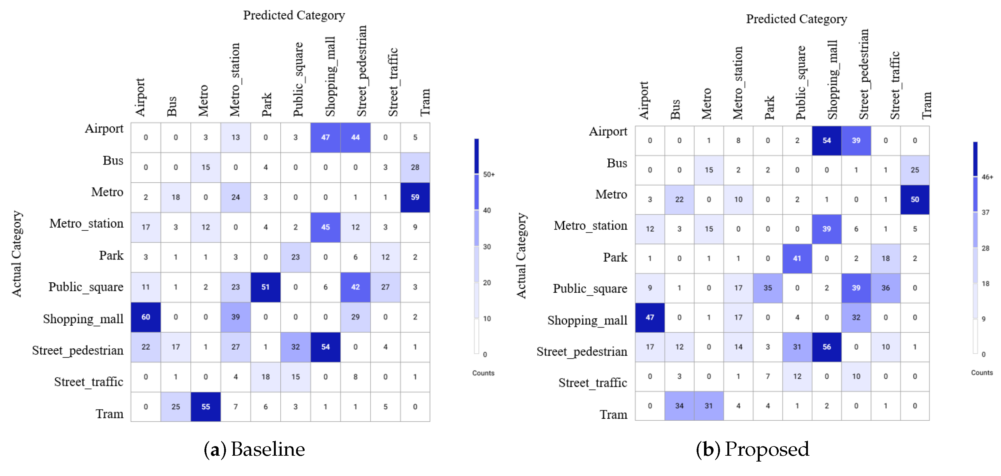
We use Mel-spectrograms with 128 Mel-filterbanks for all experiments where the number of FFT bins, window length, and shift size are set to 2048, 40 ms, and 20 ms, respectively. During the training phase, we randomly select 250 consecutive frames (5 s) instead of using the whole recording. In the test phase, we apply a test time augmentation method [25] that splits an audio recording into several overlapping sub-recordings, and the output layer’s mean is used to perform classification. This technique reportedly mitigates the overfitting described in previous works [11,26].

We use an SGD optimizer with a batch size of 24. The initial learning rate is set to 0.001 and scheduled with a warm restart of the stochastic gradient descent [27]. We train the DNN in an end-to-end fashion and employ support vector machine (SVM) classifiers to construct an ensemble system. Further technical details required to reproduce this study are provided in the author’s technical report for the DCASE 2020 challenge [28].

5. Result Analysis

Table 2. Baseline comparison with other systems. Classification accuracies reported using DCASE2020 fold1 configuration.

System	Acc (%)
DCASE2019 baseline [2]	46.5
DCASE2020 baseline [24]	51.4
Ours-baseline	65.3

compares this study’s baseline with the two official baselines from the DCASE community. The DCASE2019 baseline is fed with log Mel-spectrograms and uses convolution and fully-connected layers. Furthermore, the DCASE2020 baseline is given L3-Net embeddings [29] extracted from another DNN and uses fully-connected layers for classification. Our baseline uses mel-spectrograms as inputs, and it uses convolution, batch normalization [30], and Leaky ReLU [31] layers with residual connections [32]. We exploit SE module after each residual block (the model architecture, as well as the performance for each device and scene, are presented in [28]). The results show that our baseline outperforms the DCASE2020 baseline over 10% in terms of classification accuracy.

Table 3. Effect of LCNN, data augmentation, and deep architecture modules.

System	Config	Acc (%)
ResNet	-	65.1
ResNet(baseline)	mix-up	65.3
ResNet	SpecAug	66.7
ResNet	mix-up+SpecAug	67.3
LCNN	-	67.1
LCNN	mix-up	68.4
LCNN	SpecAug	69.2
LCNN	mix-up+SpecAug	69.4
LCNN	SE	68.0
LCNN	CBAM	68.3
LCNN	SE+CBAM	68.2
LCNN	mix-up+SpecAug+SE	69.8
LCNN (proposed)	mix-up+SpecAug+CBAM	70.4

describes the effectiveness of the proposed approaches when using the LCNN, SE, and CBAM. It also compares the effects of using the mix-up and/or specAugment data augmentation methods. First, ResNet and the LCNN achieve accuracies of 65.1% and 67.1%, respectively, without any data augmentation or deep architecture modules. To optimize the LCNN system, we also adjust the number of blocks, finding that the original LCNN with four blocks achieves the best performance. Second, we validate the effectiveness of data augmentation. The results show that mix-up and specAugment are both effective and using a combination of these two methods obtains optimal results. Third, we apply the deep architecture modules of SE and CBAM. Our analysis of the experimental results reveals that CBAM is slightly better than SE.

Figure 3 represents the confusion matrices for the entire test set and

Table 4. Comparison of errors when classifying frequently misclassified pairs of acoustic scenes between the baseline and the proposed system. Reduction refers to the number of misclassified pairs.

Class	Baseline	Proposed	Reduction
Metro-Tram	114	81	33
Shopping-Airport	107	101	6
Shopping-Metro_st	84	56	28
Shopping-Street_ped	83	88	−5
Public_square-Street_ped	74	70	4
Total	462	396	66

depicts the top five frequently misclassified pairs. There are several improvements for other misclassified pairs, but even among the top-5, we found that the total number of total misclassified pairs is reduced by 17% when compared to the baseline. The number of misclassification errors is reduced except for the pair of “shopping mall’’ and “street pedestrian’’. Interestingly, except for the pair of “shopping mall’’ and “street pedestrian’’, all other classes in each commonly misclassified pair belong to the same categories; those categories include indoor, outdoor, and public transport. Namely, Metro-Tram (public transport), Shopping-Airport (indoor), Shopping-Metro_st (indoor), Public_square-Street_ped (outdoor) have a common category in each pair, whereas shopping mall and street pedestrian are in the indoor and outdoor categories, respectively. This result shows that the proposed architecture can distinguish between the relatively similar classes when using detailed information.

Table 5. Comparison with recent studies using DCASE2020 1A development dataset.

System	Acc(%)	#Params
LCNN(Proposed)	70.4	0.85 M
Jung et al. [6]	70.3	13.2 M
Kim et al. [33]	71.6	4 M
Liu et al. [7]	70.2	3 M

describes the comparison results with the performance of the state-of-the-art systems and model complexity. It should be noted that comparisons are only conducted for a single system. Although we did not achieve the best performance, our system showed comparable results with a few parameters. As we do not exploit complex data preprocessing compared to other state-of-the-art systems, we will consider a further study with cutting-edge data preprocessing methods in the future.

6. Conclusions

In this research, we assumed that information that enables the classification of different scenes with similar characteristics might be specific and reside in small particular regions throughout the recording for the ASC task. In the case of a shopping mall and an airport, there is a common characteristic in that they are reverberant and there is a babble of voices due to being indoors, audio recordings in these locations include background noise that consists of people talking. Therefore, specific details could provide important cues to distinguish the two classes. Based on this hypothesis, we proposed a method designed to better capture this discriminative information. We applied two deep architecture modules, the LCNN and CBAM, and we also included two data augmentation methods, mix-up, and specAugment. The proposed method improved the system performance with less computation and additional parameters. We achieved an accuracy of 70.4% using the single best-performing proposed system, compared to 65.1% of the baseline.

References

1. Plumbley, M.D.; Kroos, C.; Bello, J.P.; Richard, G.; Ellis, D.P.; Mesaros, A. Proceedings of the Detection and Classification of Acoustic Scenes and Events 2018 Workshop (DCASE2018), Surrey, UK, 19–20 November 2018; Tampere University of Technology, Laboratory of Signal Processing: Tampere, Finland, 2018. [Google Scholar]
2. Mandel, M.; Salamon, J.; Ellis, D.P.W. Proceedings of the Detection and Classification of Acoustic Scenes and Events 2019 Workshop (DCASE2019), New York, NY, USA, 25–26 October 2019; New York University: New York, NY, USA, 2019. [Google Scholar]
3. McDonnell, M.D.; Gao, W. Acoustic scene classification using deep residual networks with late fusion of separated high and low frequency paths. In Proceedings of the ICASSP 2020-2020 IEEE International Conference on Acoustics, Speech and Signal Processing (ICASSP), Barcelona, Spain, 4–8 May 2020; pp. 141–145. [Google Scholar]
4. Pham, L.; Phan, H.; Nguyen, T.; Palaniappan, R.; Mertins, A.; McLoughlin, I. Robust acoustic scene classification using a multi-spectrogram encoder-decoder framework. Digit. Signal Process. 2021, 110, 102943. [Google Scholar] [CrossRef]
5. Jung, J.W.; Heo, H.S.; Shim, H.J.; Yu, H.J. Knowledge Distillation in Acoustic Scene Classification. IEEE Access 2020, 8, 166870–166879. [Google Scholar] [CrossRef]
6. Jung, J.W.; Shim, H.J.; Kim, J.H.; Yu, H.J. DCASENet: An integrated pretrained deep neural network for detecting and classifying acoustic scenes and events. In Proceedings of the ICASSP 2021-2021 IEEE International Conference on Acoustics, Speech and Signal Processing (ICASSP), Toronto, ON, Canada, 6–11 June 2021; pp. 621–625. [Google Scholar]
7. Liu, Y.; Zhou, X.; Long, Y. Acoustic Scene Classification with Various Deep Classifiers. In Proceedings of the DCASE2020 Challenge, Virtually, 2–4 November 2020. Technical Report. [Google Scholar]
8. Gharib, S.; Drossos, K.; Cakir, E.; Serdyuk, D.; Virtanen, T. Unsupervised adversarial domain adaptation for acoustic scene classification. arXiv 2018, arXiv:1808.05777. [Google Scholar]
9. Primus, P.; Eitelsebner, D. Acoustic Scene Classification with Mismatched Recording Devices. In Proceedings of the DCASE2019 Challenge, New York, NY, USA, 25–26 October 2019. Technical Report. [Google Scholar]
10. Kosmider, M. Calibrating neural networks for secondary recording devices. In Proceedings of the Detection and Classification of Acoustic Scenes and Events Workshop (DCASE), New York, NY, USA, 25–26 October 2019; pp. 25–26. [Google Scholar]
11. Heo, H.S.; Jung, J.W.; Shim, H.J.; Yu, H.J. Acoustic Scene Classification Using Teacher-Student Learning with Soft-Labels. arXiv 2019, arXiv:1904.10135. [Google Scholar]
12. Jung, J.W.; Heo, H.; Shim, H.J.; Yu, H.J. Distilling the Knowledge of Specialist Deep Neural Networks in Acoustic Scene Classification. In Proceedings of the Detection and Classification of Acoustic Scenes and Events 2019 Workshop (DCASE2019), New York, NY, USA, 25–26 October 2019; pp. 114–118. [Google Scholar]
13. Wu, X.; He, R.; Sun, Z. A Lightened CNN for Deep Face Representation. arXiv 2015, arXiv:1511.02683. [Google Scholar]
14. Maaten, L.V.D.; Hinton, G. Visualizing data using t-SNE. J. Mach. Learn. Res. 2008, 9, 2579–2605. [Google Scholar]
15. Wu, X.; He, R.; Sun, Z.; Tan, T. A light cnn for deep face representation with noisy labels. IEEE Trans. Inf. Forensics Secur. 2018, 13, 2884–2896. [Google Scholar] [CrossRef] [Green Version]
16. Lavrentyeva, G.; Novoselov, S.; Tseren, A.; Volkova, M.; Gorlanov, A.; Kozlov, A. STC antispoofing systems for the ASVSpoof2019 challenge. arXiv 2019, arXiv:1904.05576. [Google Scholar]
17. Lai, C.I.; Chen, N.; Villalba, J.; Dehak, N. ASSERT: Anti-Spoofing with squeeze-excitation and residual networks. arXiv 2019, arXiv:1904.01120. [Google Scholar]
18. Zhang, H.; Cisse, M.; Dauphin, Y.N.; Lopez-Paz, D. mixup: Beyond empirical risk minimization. arXiv 2017, arXiv:1710.09412. [Google Scholar]
19. Park, D.S.; Chan, W.; Zhang, Y.; Chiu, C.C.; Zoph, B.; Cubuk, E.D.; Le, Q.V. SpecAugment: A Simple Data Augmentation Method for Automatic Speech Recognition. arXiv 2019, arXiv:1904.08779. [Google Scholar]
20. Hu, J.; Shen, L.; Sun, G. Squeeze-and-excitation networks. In Proceedings of the IEEE Conference on Computer Vision and Pattern Recognition, Salt Lake City, UT, USA, 18–22 June 2018; pp. 7132–7141. [Google Scholar]
21. Woo, S.; Park, J.; Lee, J.Y.; So Kweon, I. Cbam: Convolutional block attention module. In Proceedings of the European Conference on Computer Vision (ECCV), Munich, Germany, 8–14 September 2018; pp. 3–19. [Google Scholar]
22. Goodfellow, I.J.; Warde-Farley, D.; Mirza, M.; Courville, A.; Bengio, Y. Maxout networks. arXiv 2013, arXiv:1302.4389. [Google Scholar]
23. Mun, S.; Park, S.; Han, D.K.; Ko, H. Generative adversarial network based acoustic scene training set augmentation and selection using SVM hyper-plane. In Proceedings of the Detection and Classification of Acoustic Scenes and Events 2017, Munich, Germany, 16 November 2017; pp. 93–97. [Google Scholar]
24. Heittola, T.; Mesaros, A.; Virtanen, T. Acoustic scene classification in DCASE 2020 Challenge: Generalization across devices and low complexity solutions. In Proceedings of the Detection and Classification of Acoustic Scenes and Events 2020 Workshop (DCASE2020), Virtually, 2–4 November 2020. [Google Scholar]
25. Nagrani, A.; Chung, J.S.; Xie, W.; Zisserman, A. Voxceleb: Large-scale speaker verification in the wild. Comput. Speech Lang. 2020, 60, 101027. [Google Scholar] [CrossRef]
26. Jung, J.W.; Heo, H.S.; Shim, H.J.; Yu, H.J. DNN based multi-level feature ensemble for acoustic scene classification. In Proceedings of the Detection and Classification of Acoustic Scenes and Events 2018 Workshop (DCASE2018), Surrey, UK, 19–20 November 2018; pp. 113–117. [Google Scholar]
27. Loshchilov, I.; Hutter, F. Sgdr: Stochastic gradient descent with warm restarts. arXiv 2016, arXiv:1608.03983. [Google Scholar]
28. Shim, H.J.; Kim, J.H.; Jung, J.W.; Yu, H.J. Audio Tagging and Deep Architectures for Acoustic Scene Classification: Uos Submission for the DCASE 2020 Challenge. In Proceedings of the DCASE2020 Challenge, Virtually, 2–4 November 2020. Technical Report. [Google Scholar]
29. Cramer, J.; Wu, H.H.; Salamon, J.; Bello, J.P. Look, Listen and Learn More: Design Choices for Deep Audio Embeddings. In Proceedings of the ICASSP 2019-2019 IEEE International Conference on Acoustics, Speech and Signal Processing (ICASSP), Brighton, UK, 12–17 May 2019; pp. 3852–3856. [Google Scholar]
30. Ioffe, S.; Szegedy, C. Batch Normalization: Accelerating Deep Network Training by Reducing Internal Covariate Shift. In Proceedings of the International Conference on Machine Learning, Lille, France, 6–11 July 2015; pp. 448–456. [Google Scholar]
31. Maas, A.L.; Hannun, A.Y.; Ng, A.Y. Rectifier nonlinearities improve neural network acoustic models. Proc. icml 2013, 30, 3. [Google Scholar]
32. He, K.; Zhang, X.; Ren, S.; Sun, J. Deep residual learning for image recognition. In Proceedings of the IEEE Conference on Computer Vision and Pattern Recognition, Las Vegas, NV, USA, 27–30 June 2016; pp. 770–778. [Google Scholar]
33. Yang, D.; Wang, H.; Zou, Y. Unsupervised Multi-Target Domain Adaptation for Acoustic Scene Classification. arXiv 2021, arXiv:2105.10340. [Google Scholar]
Figure 1. t-SNE embedding visualization results. (a,b) illustrate the expressiveness of the baseline classifying devices and scenes, respectively. Color dots represent the classes.
Applsci 11 08361 g001
Figure 2. Comparison of ReLU activation function (a) and MFM (b). Orange, green, and white indicate negative, positive, and zero values, respectively. ReLU removes all negative values, while MFM considers the element-wise maximum.
Applsci 11 08361 g002
Figure 3. Confusion matrices for comparing frequently misclassified pairs of classes. The numbers in the box describe the mismatch between actual and predicted classes. The darker colors indicate more confusion.
Applsci 11 08361 g003