1. Introduction
The supply of energy and drinking water is a fundamental aspect of the sustainable development of cities and societies, but it is limited by various factors with complicated relationships. Climate change has restricted the ability to supply drinking water, and concerns about greenhouse gas emissions have catalyzed a worldwide interest in improving energy efficiency [
1,
2]. In addition, population growth increases water and energy demands in various sectors, including the household sector [
3]. Due to water–energy interactions, there is potential for synergy between the two sectors. Therefore, the nexus between them and the importance of integrated water and energy planning are important research topics [
4,
5].
Water distribution networks (WDNs), which transmit water to consumers after physical and chemical treatment, are vital parts of water supply systems. The role of WDNs is amplified when there is a demand for higher water pressure, as this leads to the implementation of domestic pumps that consume a significant amount of energy. Various studies have examined the design of WDNs through different approaches, such as cost minimizing [
6], contamination control [
7], energy recovery [
8], and flexible designs using multi-objective optimization [
9,
10]. Several cost-related factors (e.g., leaks, pipe breaks, water network repair, and the energy required to pump water into the network) are generally considered by all water companies. Analyses of such factors have revealed the significant role of network pressure on the operation of WDNs [
11,
12]. Pressure is an adjustable parameter that, if manipulated correctly, can reduce the maintenance costs of water companies.
Using local field data, Ghorbanian et al. [
13] proposed a probabilistic approach that considers uncertain demands and pipe roughness to determine the effects of pressure on burst frequency. The Monte Carlo method was used to implement this probabilistic approach in the water network of Hamilton, Ontario, Canada. Due to the significant effect of pressure reduction on burst frequency, they proposed to re-evaluate pressure standards for WDNs.
Chang et al. [
14,
15] proposed a head out flow relationship (HOR) modeling approach which takes into account the residential environment of consumers and various water-supply methods. The robustness of this method is assessed by selecting two demonstration blocks and evaluating the available flow rate supplies under abnormal conditions. This method provides a reliable pressure-driven analysis by applying a rational and objective HOR selection procedure.
Water leakage in WDNs, the relationship between water leakage and pressure, and the methods for detecting leaks have been widely researched [
16]. Because leakage plays a vital role in water loss and non-revenue water, water companies have tried to reduce leakage by replacing pipes, implementing leakage detection strategies, and reducing pressure in WDNs [
17].
Pressure reducing valves (PRVs) automatically reduce high inlet pressure to a steady and low level of downstream pressure [
18]. The utilization of PRVs has become a common method for pressure management in the WDNs. There are two major categories of applying management commands and adjusting these valves: mechanical control and electronic control [
17].
In mechanical control, adjustment of PRV is generally manual. These valves work even in changing flow rate or varying inlet pressure and for many years, have been used to reduce service pressure to an appropriate level. The setting of these valves can be adjusted to meet the demand alterations of the system, but they cannot be adjusted continuously in real time. Therefore, pressure management in this mechanical control method is on a daily or monthly basis [
19]. In recent years, because of the advancements of electronic technologies and control algorithms, mechanical control and conventional PRVs have become obsolete [
20]. The beforementioned advancements have led to the widespread utilization of electronic actuators, which are capable of providing better performance and are considered to be an intelligent pressure management method of the WDN in many studies [
21]. There are three main categories of electronic control PRV: time-modulated, flow-modulated, and remote node-based modulation.
In time-modulated mode, time changes are the basis for applying the pressure adjustment pattern by the operator. In this mode, the flow rate changes are not taken into account. The goal of pressure management in this mode is to supply the anticipated value for upstream pressure [
19].
Flow-modulated mode uses the flow through the node for adjusting pressure. In this mode, the flow–pressure relationship adjustment is used to provide the desired amount of flow supplied to the node throughout the pressure management period [
22].
In remote node-based modulation mode, one of the network nodes, generally the critical node, is considered as the control node. The pressure is managed in a way that the desired pressure in this control node is provided [
23].
Different methods have been employed to specify the best locations for installing PRVs in WDNs. Such methods include probabilistic approaches and deterministic optimization algorithms [
24]. For almost all the techniques used for analyzing pressure management, modeling the WDN is the first step. This step is conducted using various software packages, such as EPANET. Thornton et al. have also developed a method to evaluate the effects of pressure management in a WDN without the need for WDN modeling [
25].
Many articles have realized economic analyses of the operating and maintenance costs associated with WDNs. For example, Kanakoudis and Tolikas [
26] proposed a model for calculating the optimum replacement time of pipes in a water network, based on the costs of repairing pipe failures and leaks. They concluded that the optimum replacement time for the city of Athena is 69 years after installation. Their techno-economic model considers many kinds of costs related to the repair and replacement of the trouble-inducing parts of a WDN.
Mann and Frey [
27] presented a framework that assesses water pipe degradation over time, which increases the operating and maintenance costs of water utility companies throughout the life cycle of pipes. They proposed that the cost-effectiveness of any WDN-related investment could be determined by calculating a risk score for all pipes based on the likelihood of pipe failure.
Creaco and Walski [
28] presented an economic analysis that assesses the consequences of reducing pressure using PRVs or real-time control (RTC) on leakage and burst frequency. They concluded that as long as the operating and maintenance costs are low, there is no need to use PRVs or RTC. When the costs increase, the first option should be to introduce PRVs, then RTC.
Energy consumption in water supply systems has led many researchers to look for more integrated approaches to water and energy. In one study, energy consumption in WDNs was evaluated through a life-cycle analysis of water network in three stages (fabrication, use, and disposal), and it was concluded that pipe replacements with a frequency of 50 years result in the lowest amount of energy consumption [
29]. In addition, many articles have investigated the water–energy nexus for WDNs, specifically on the energy consumed by pumping stations for water transmission and distribution [
30,
31,
32]. The main aim of these studies was to respond to demand through pump scheduling [
33].
Hashemi et al. [
34] optimized the performance of a variable-speed pump using an ant-colony algorithm. Using this system, they increased the flexibility of the pumping station, regarding the water demand changes during a day and obtained the pumping schedule that optimized energy costs. Because of the importance of demand variation during daytime hours for pump scheduling, Giustolisi et al. [
35] proposed different scenarios for predicting demand variation to optimize the performance of pumps. Furthermore, Abdallah and Kapelan [
36] proposed an optimization method for the energy consumption of fixed speed and variable speed pumps regarding the nonlinear behavior of water flow.
Colombo et al. [
37] presented an economic approach based on energy costs of leakage in WDNs, using EPANET, to investigate the importance of energy costs when the pipes leak. Shao et al. [
38] also studied the scheduling of pumps and PRVs in WDNs to illustrate that pressure management reduces leakage and energy consumption by 33.4% and 25.4%, respectively.
The relationship between water network pressure and the energy consumed by domestic WPBSs to supply water and maintain pressure in a building pipeline remains to be assessed. WPBSs are one of the greatest energy-consuming components in buildings, and the pressure provided by water companies significantly affects the amount of energy that they consume. In this paper, the pressure supplied for each consumer was calculated using EPANET, which models water distribution systems based on the elevation and base demand of each node. The supplied pressure fluctuation was vital when calculating energy consumption. Therefore, the head driven simulation method (HDSM) was used when considering the explicit relationship between the pressure and the nodal outflow. The relationships of leakage and burst frequency with pressure were implemented in the model to calculate changes in operation and maintenance costs. After determining energy consumption by WPBSs, the objective function was defined. The model was used to calculate the daily and hourly optimized pressures and optimized total costs for the city of Baharestan. To evaluate the impact of input variables uncertainties on the daily optimized pressure and cost, a sensitivity analysis was conducted.
2. Materials and Methods
2.1. WDN Simulation
The present hydraulic analysis of WDN aims to calculate indefinite parameters, such as the flow rate, the velocity, and the pressure of nodes, using input data related to these parameters. Both the energy equation and the continuity equation must be considered when analyzing WDN from a hydraulic perspective. According to the continuity equation, the mass flow rate in a pipe must remain constant at a steady-state condition. In addition, the energy equation determines the amount of energy head loss on the two sides of a pipe as a function composed of characteristics related to the flowing fluid, the specifications of the pipe, and the features of the flow (flow rate or velocity). Moreover, the Hazen–Williams, Darcy–Weisbach, and Manning relations are often used to determine the energy head loss in a pipe.
Some of the equations used to analyze WDNs are nonlinear and iteration processes are used to solve them. The most common procedure is the gradient method. This procedure is the basis of the analyses carried out by many software programs in this field, including EPANET. With this method, there is no need to make an initial estimation of the flow rate in the pipes or the head of the nodes because the improved values of the flow rate and heads are directly used in each iteration. Although more equations need to be solved when using this method, its computational robustness is much higher in comparison to other methods [
39].
Many software packages have been developed for the hydraulic analysis of WDNs. EPANET 2.0 is the most well-known and commonly used and it is used in this study also because of its open-source design and its extensive set of developed lateral tools. For example, EPANET can connect to the programming environment of technical computing software, while it can also exploit both the demand-driven simulation method (DDSM) and the HDSM in the hydraulic analysis of networks.
In the DDSM, it is assumed that the demands are fixed and known in advance, regardless of nodal pressure variations. However, this assumption is only acceptable under normal conditions and when the existing pressure meets the minimum pressure required by the consumer. It cannot satisfy systems with pressure lower than the required value at some nodes [
40].
The relationship between the actual supplied flow rate and the pressure in each node is taken into account in the HDSM. Research in this field, in the last three decades, has proven the dependency of the output flow rate on the pressure of the nodes [
41,
42,
43,
44]. Due to the importance of the pressure of each node for computing the consumed energy in domestic WPBSs, this study uses the HDSM to properly account for pressure alterations and evaluate the hydraulic parameters of nodal heads and velocity in pipes more realistically than DDSM. To conduct a pressure-based hydraulic analysis of the networks, the available discharge of a node should not be considered constant (
). The mentioned value must be computed by Equation (1) based on the existing pressure of the node (
) [
44].
In this formula, is the demand or required discharge at node j, is the available discharge at node j, is the available head at node j, is the minimum required head (for heads greater than , demand or required discharges are supplied completely, and in fact this is the minimum design head), is the minimum head (for heads lower than this, the available discharge is zero), is the threshold head (for values greater than this, the discharge does not change with head and remains constant), n is the head exponent, is the volumetric portion of the available release, and is the head-dependent portion of the available discharge.
Assuming a half-inch and fully open faucet, the Equation (1) can be rewritten by applying the values suggested by Shirzad and Tabesh [
45]. In this regard, the following numbers can be assumed:
,
,
,
, and we can conclude that:
To conduct the HDSM analysis, EPANET is connected to a technical computing programming environment to modify different parameters [
46,
47,
48]. In this study, the elevation of the reservoir was altered in order to analyze the effects of the average pressure of WDN (
) on operating and maintenance costs and the cost of energy consumed by domestic WPBSs. The results of this phase are the hourly pressure and available discharge of nodes during a day, in addition to the water pressure at different points of the network, used in the following analyses.
2.2. Water Leakage Simulation
One of the main results of altering the average pressure of the WDN is reducing the leakage. Water leakage is the main reason for real water loss, and reducing it presents a potential for water companies to reduce their costs and save water, especially in cases of potable water scarcity. Numerous methods are proposed to investigate the effects of pressure variation on leakage [
49]. In addition, the calibration of leakage in WDNs using pressure driven analysis to minimize the differences between field measurements and simulation results [
50], and a physically based approach to support leakage management plans [
51] has been the subject of some recent papers. The fixed and variable area discharges (FAVAD) equation is amongst the most well-known methods [
52] and provides useful insights into the behavior of real networks [
53].
where
is the water leakage after pressure reduction (m
3)
, is the water leakage before pressure reduction (m
3),
is the pressure before reduction (mH
2O),
is the pressure after reduction (mH
2O), and
is the leakage exponent, which depends on the type of failures and the pipe material. According to experimental studies, the value of
is estimated between 0.5 and 2.5 [
54] and can be calculated with an experimental study on the studied network.
Figure 1 illustrates the relationship between the pressure and leakage for different values of
.
2.3. Burst Frequency Simulation
The reduction of burst frequency can significantly reduce the operating and maintenance costs. The costs of repairing bursts includes pipe and couplings used for fixing, personnel, equipment, and machinery that incline water companies to reduce the average pressure of WDN. Burst frequency generally depends on the pipe age, pipe material, external load, and climate conditions. Different models are developed to investigate this dependency [
13]. Lambert et al. developed the following equation [
55]:
In this formula, BF0 is the burst frequency before pressure management, is the burst frequency after pressure management, is the non-pressure dependent burst frequency, H1 is the operating pressure after pressure management, is the operating pressure before pressure management, and is the burst exponent calculated experimentally, according to the studied network.
2.4. Energy Consumption Simulation for Domestic Water Pressure Booster Systems
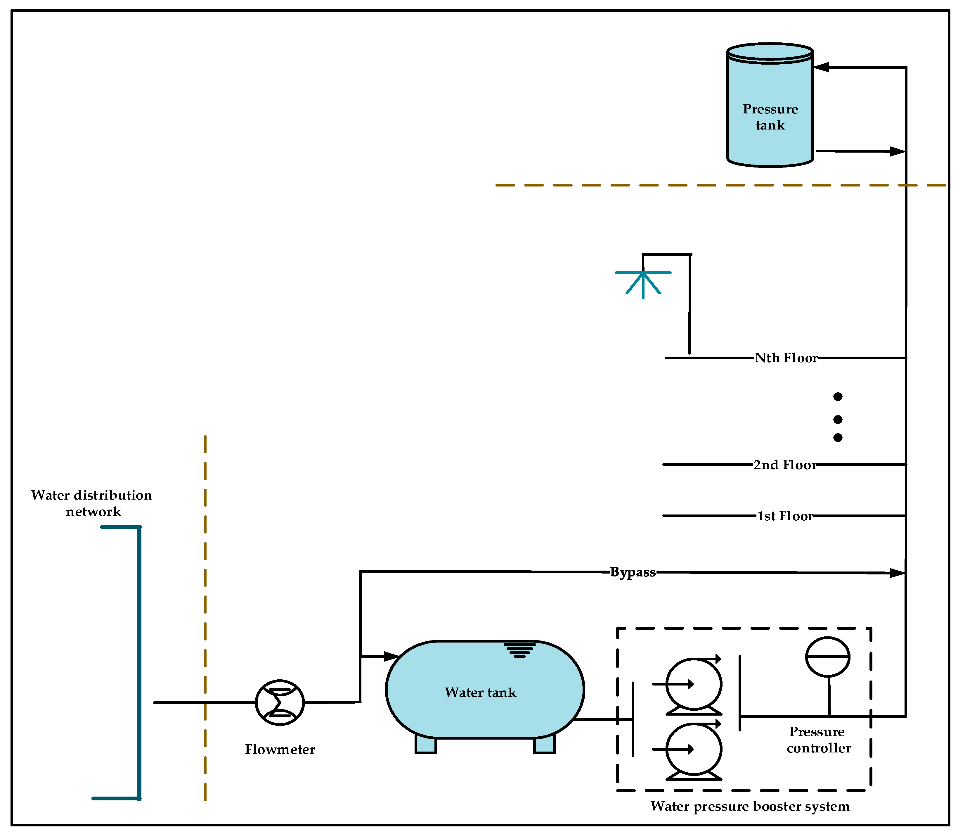
WPBSs are used wherever there is a need to increase pressure and are responsible for supplying water and maintaining water pressure in the pipelines of a building [
56]. WPBSs are widely installed in houses and apartments around the world to increase water pressure and provide the flow required by consumers (which the water company is not able to provide) on different floors throughout the day. Different designs for installing WPBSs have been proposed for domestic water supply systems, based on different local rules and standards.
Figure 2 presents the design of a typical domestic water supply system proposed by booster pump producer companies [
57].
In most designs, the water storage tank is located on the ground floor. Water can be stored in these tanks during off-peak hours, during which the water provided by water companies exceeds the level of consumption. The stored water can then be used during peak hours to meet the flow requirements of consumers using WPBSs. A WPBS increases the pressure of the water stored in the tank through a conduit and includes one or more pumps that are designed and selected according to the height of the building, a booster pump controller, and a pressure sensor affixed to the exit side of the booster pump and connected to the control device. The controller switches off any number of pumps when they reach the predetermined upper-pressure limit and switches on when the lower pressure limit is reached. The pressure tank can be installed on the roof to satisfy the demands imposed on the system. Without the pressure tank, the booster would restart upon the slightest call for flow—for example, due to a small leak in the piping system.
A typical energy-saving strategy is to install a bypass connection to use the pressure provided by the water company for the domestic water supply system that reduces the need to start the WPBS. The higher the supply of pressured water from water companies is, the lower the energy consumption of the WPBS will be.
The power required for the pump to lift an amount of liquid at a particular height is called hydraulic power and is calculated by Equation (5).
In this equation, P is the power consumption, ρ is the water density, g is the acceleration of the gravity, Q is the water discharge, η is the pump efficiency, and h is the pumping head and it is calculated according to the Equation (6).
In this formula,
is the head supplied to the faucet by the pump,
is the faucet elevation relative to the pump,
is the piping friction losses, and
is the suction pressure. Suction pressure can be regarded as the water pressure supplied by the water company, which equals
and its calculation is shown in
Section 2.1.
The efficiency of the pump η can be calculated using Equation (7).
When the pumping head h is negative, the pressure supplied by the water company is enough for the building’s consumers. In this case, there is no need for the WPBS, and no additional energy is consumed.
The energy efficiency varies according to the production or installation conditions [
58]. Many researchers have focused on energy efficiency enhancement opportunities. Several strategies, such as controlling the speed of the pumping system using variable frequency drives [
59], installing parallel pumping systems [
60], increasing the diameter of the piping system [
61], and selecting an appropriate pumping system by minimizing total horsepower [
59], have been proposed.
Building designers select the WPBS that will meet the total flow requirements of the consumers, while , , and have the maximum available values according to the building’s piping system and has the minimum value. In this situation, designers select the WPBS that will maximize the system’s efficiency. Any changes to the parameters will affect the optimum operating point and will reduce the efficiency of the system. Installing parallel pumps can reduce this problem in some buildings.
2.5. Optimization Method
Water companies are able to alter the pressure of the whole WDN of a city or a specific zone by installing PRV or pumping stations, which reduce or increase the average pressure of the affected zone. Decreasing will reduce the operating and maintenance costs of the WDN and will also decrease for each node, leading to an increase in the operating costs of WPBS. On the other hand, increasing Have will increase the operating and maintenance costs of the WDN and will also increase for each node, leading to a decrease in the operating costs of WPBS. These conflicting interests between water companies and water consumers call for an integrated water and energy approach to facilitate optimal decisions regarding the WDN average pressure in any zone of the city based on local conditions. To do this, the costs of the water sector and the energy sector related to altering the average pressure must be analyzed.
According to
Section 2.2, the cost of energy consumed by WPBS can be calculated using the following equation:
In this formula,
is the operating cost of the WPBS and
is the price of energy. In addition, the operating and maintenance cost of a WDN, which is affected by altering
, can be calculated using the following equation:
In this formula,
is the operating and maintenance cost of the WDN,
is the cost of repairing pipe burst, and
is the price of water. Finally, the optimum pressure point for
is calculated by the following equation:
In this objective function, j is the number of nodes of the WDN. is the decision variable, which in practice can be changed by installing PRV. The mentioned constraint limits the available pressure of each node that the water company provides. and denote the minimum and maximum allowable pressure heads at the consumption nodes, respectively. Since the water demand and energy price vary throughout a day, the optimization equation calculates hourly water and energy costs over 24 h.
3. Case Study
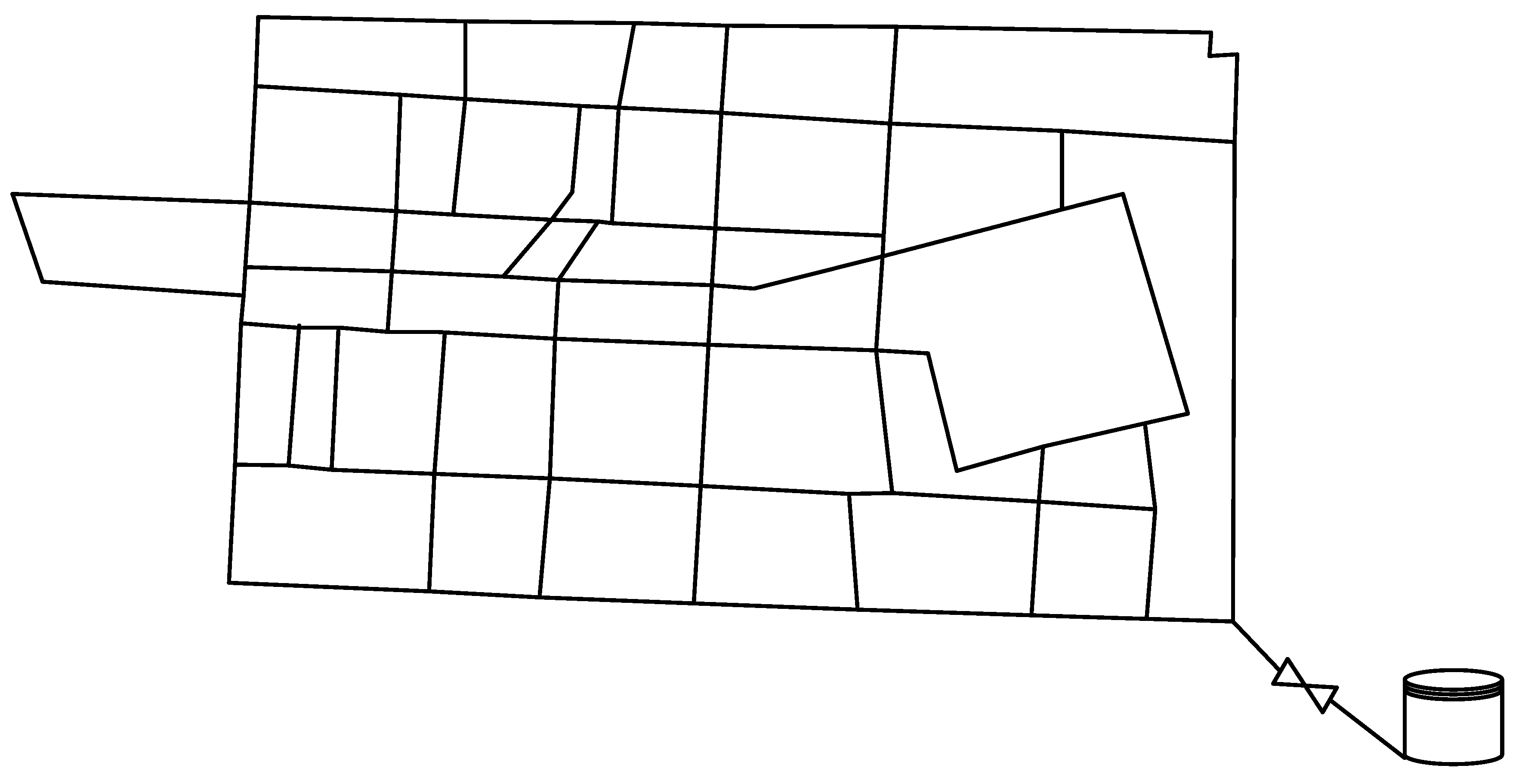
The network of Baharestan city, located in the Isfahan province of Iran, was investigated to illustrate the potential of the developed model to establish a water–energy nexus based on local factors. This network consists of 71 nodes, 107 pipes, 1 reservoir, and 1 PRV for altering the average pressure of the network. The characteristics of the nodes and pipes are presented in
Table 1 and
Table 2, respectively.
To calibrate the pipe roughness coefficient and nodal demand of the hydraulic model, the genetic algorithm was applied based on the following steps [
62]:
Preparation of hydraulic parameters of the existing water network (information of nodes and network pipes).
Implementing genetic algorithm for determining the parameters with uncertainty.
Conducting the optimization process for calibration by calculating the mean absolute percentage error (MAPE) using Equation (11).
In this formula, m is the number of data, and and are the measured and simulated value of considered parameters at point i.
- 4.
Comparing the empirical and calculated results at each iteration.
- 5.
Calculating the objective function and finally obtaining the optimal solution in which the defined conditions for calibration is satisfied.
This process was performed using two consumption scenarios (normal and fire flow). To calculate the considered variables (Hazen–Williams roughness coefficient and nodal demand), pressure head measurements at 20 nodes for Baharestan water network were used for EPANET calibration. The MAPE factor was used to evaluate the results. Based on the results, the Hazen–Williams coefficient was estimated to be 130. The schematic of the network is presented in
Figure 3.
The data needed to run the water section of the model were gathered (
Table 3). The values of some parameters (e.g., leakage in the basic situation, burst frequency in the basic situation, leakage exponent, burst exponent, and the base demand of each node and related information) were gathered from data of previous years. These data and the data used for calibration were gathered through a long-term monitoring of flowmeters, water pressure loggers, and basic operating and hydraulic information of the entire WDN.
The supplied water for 79023 inhabitants in the Baharestan city is distributed through the network to each house. The total length of pipelines is about 511 km and the total number of subscribers is 23,254 (75.2% are residential). The per capita water consumption was 278 L per day in 2020. Based on the location of each subscriber, its basic demand is attributed to the closest node in the EPANET software.
The data relating to the water pipe bursts were collected from 2016 to 2020. These data include the number of pipe bursts, and the average time and cost for repairing bursts for main, sub-main, and branch pipes. The water consumption data of five years (2016–2020), which were collected using 23,254 flowmeters, were used to calculate water loss. In addition, the data of inflow to the network (flow from reservoir node) were gathered at the same time. Pressure monitoring was conducted using 20 water pressure loggers which are distributed in the WDN. The collected data were used to calibrate the model and calculate parameters in the FAVAD and burst frequency equations.
Considering the basic state in which L0 and BF0 were measured for this situation, the average and standard deviation of daily water pressure and water flow for each node were 45 ± 17 mH2O and 5.4 ± 4.2 L/s, respectively. The lowest and highest water pressure were 5.6 mH2O and 77.7 mH2O related to node11 (at 7 p.m.) and node 18 (at 4 a.m.), respectively. Moreover, the lowest and highest water flows were 0.25 L/s and 21.17 L/s related to nodes 5, 41, 59, 61, 67 (at 4 a.m.), and node 14 (at 7 p.m.), respectively.
The model calculates the optimum average pressure of the network based on hourly intervals. The consumption coefficient for each hour was obtained, according to
Figure 4 [
63]. Fluctuations in demand throughout a day significantly affect
for each node and, in turn, the power consumed by the WPBSs.
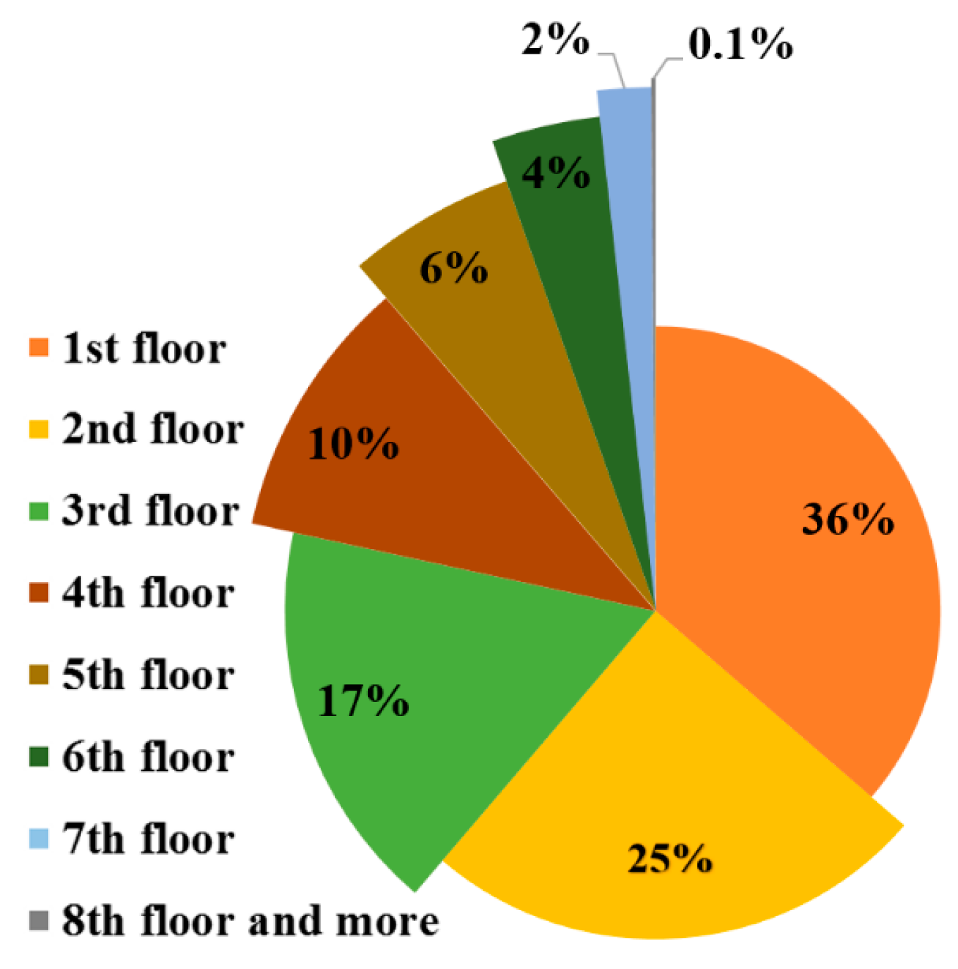
Several types of information were considered by the model when calculating the amount of energy consumed by the WPBSs. This information included the number of buildings, the corresponding floor numbers, and the number of people living on each floor.
Table 4 represents the values of the parameters related to running the energy section of the proposed model.
Figure 5 illustrates the share of people that live on different floors of the buildings in Baharestan city. To collect the required data for energy sector, Iran’s population and housing census data that were collected by Statistical Centre of Iran were used [
64]. Moreover, the WPBSs data were collected by field survey.
4. Results and Discussion
4.1. Daily Pressure Optimization
In order to manage the pressure for achieving daily optimum results, the mechanical control method was used in this section. Because there is no need to consider continuous alterations of pressure in this mode and the optimum results are required on daily basis, the mechanical control method was applied to PRV.
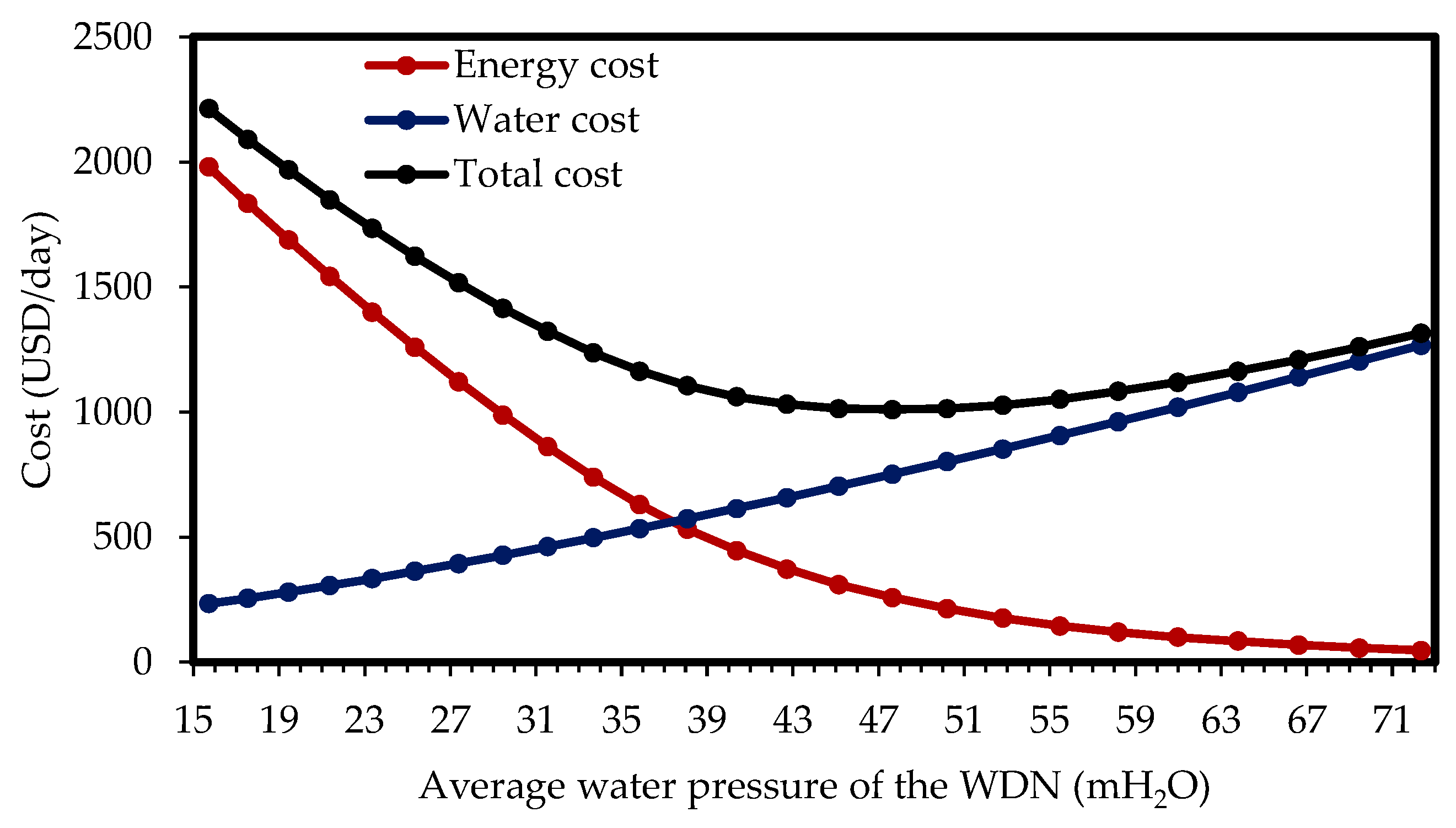
The results of the attempt to find an optimum water network pressure value are presented in
Figure 6. According to this figure, as the average water pressure of the network increases, the energy consumed by the WPBSs decreases, while leakage and burst frequencies increase. According to the model, the optimum average daily water pressure of the WDN in the city of Baharestan is 47.6 mH
2O. By adopting this pressure, the daily energy-consumption cost of the WPBS, combined with the operation and maintenance costs of the WDN, would total USD 1009. If the pressure adopted were lower, the operating and maintenance costs would decrease, while the energy consumed by the WPBSs would significantly increase. This shows the importance of using an integrated approach towards water and energy regarding the average pressure of the water network.
The determined optimum pressure level is highly dependent on local conditions. The degradation of water pipes results in a reduction of the optimum pressure of a WDN. Managing water pressure becomes increasingly important as pipes age. In addition, over time, existing slums will be replaced by multi-story buildings, which will increase the optimum average pressure. Clearly, the complicated impact of any change in local conditions on water and energy price on the optimum pressure requires policymakers to employ a dynamic approach to the challenge.
The sensitivity analysis was used in this study to assess the influence of input variables uncertainties on the daily optimized pressure and daily optimized cost. Water and energy price, leakage exponent, WPBSs efficiency, the height of buildings, and leakage were the selected parameters to be analyzed. The range of each parameter was defined based on price policy, historical data, and physical attributes of the water distribution network and WPBSs. Once the parameters were set, the model was run, and the optimized cost and optimized average water pressure of the WDN were calculated.
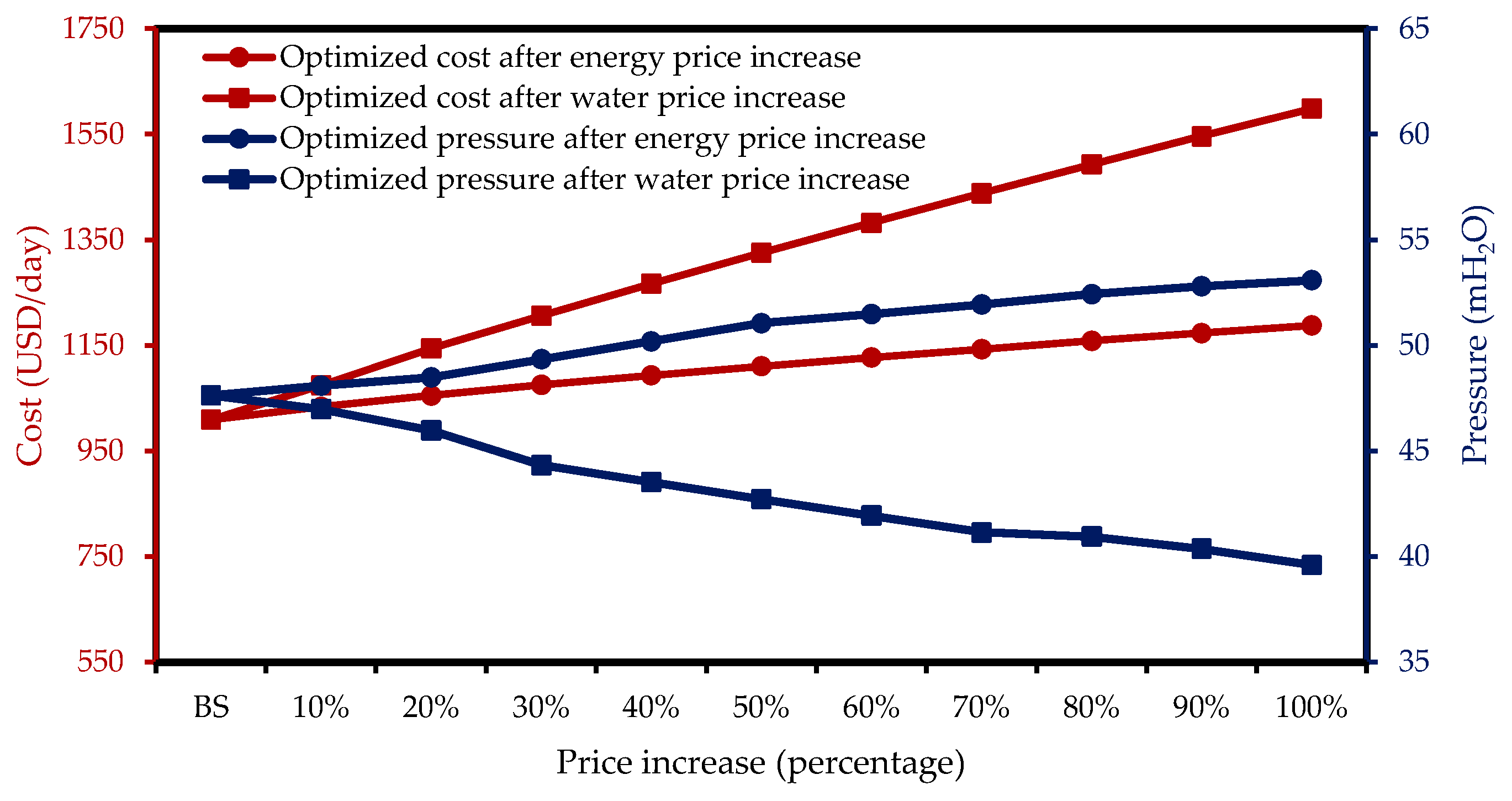
Figure 7 depicts the sensitivity of optimized cost and pressure to the changes in energy and water prices. Water and energy prices are determined by policymakers at the macro level and are generally dependent on economic, social, and political conditions. These two factors were imposed into the developed model. Considering the implantation of price adjustment policies to cut the water and electricity subsidies, it is likely that water and electricity prices will rise in the years to come. The increase in water and energy prices will decrease and increase optimized pressure, respectively. Moreover, as it is shown in the figure, the sensitivity of the optimized cost to the increase of energy is higher in comparison to the water price increase.
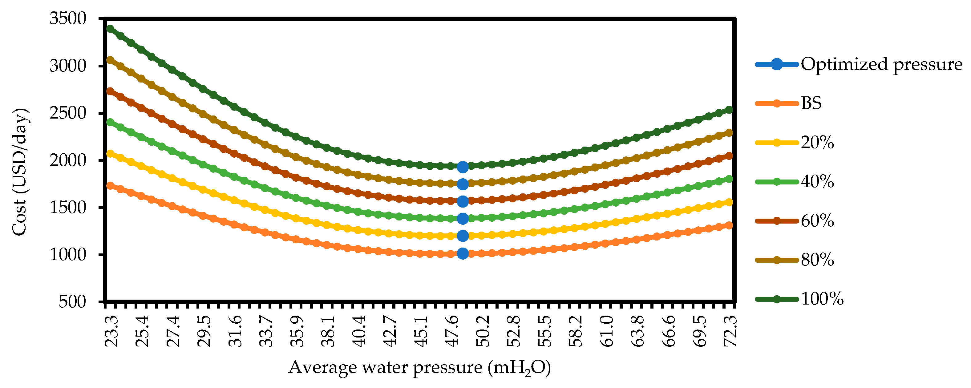
As it is illustrated in
Figure 8, with a simultaneous increase of water and energy prices, the minimum price will be in the first optimized pressure and does not change. In addition, it can be expressed that 50% and 100% simultaneous increase in water and energy prices will result in a 46% and 92% increase in optimized cost, respectively.
In the FAVAD equation, the leakage exponent has a remarkable impact on determining leakage amount considering pressure alterations and is particularly calculated empirically. The influence of this parameter generally is not taken into account in the evaluations of pressure management impact. The value of this parameter is reported between 0.5 and 2.5 in different studies. As it is described in
Table 3, the value of this parameter was considered 1.4 in the present study.
Figure 9A shows the investigation of the sensitivity of optimized results on this parameter. It was deduced that the sensitivity of optimized pressure to the alterations of this parameter is low, but the remarkable point is the sensitivity of optimized cost. The sensitivity of optimized cost to this parameter was more than any other five parameters assessed in this study. This shows the importance of precise calculation of this parameter using empirical data.
WPBS efficiency is a parameter that policymakers can use to decrease costs by providing necessary education and investments. Different operating circumstances will result in booster pumps to get out of their designed performance conditions. This will lead to a considerable decrease in the efficiency of this system. Therefore, the appropriate and comprehensive design of WPBSs will likely have a major impact on the system’s efficiency improvement.
Figure 9B shows the sensitivity of optimized results on WPBSs efficiency. An increase in WPBSs efficiency can lead to a decrease in optimized pressure, and therefore in water section costs, and as a result, the optimized cost will decrease. If the WPBSs’ efficiency increases by 20%, optimized pressure and cost will decrease by 17% and 16%, respectively.
Considering the limitations and price of land in recent years, investors and policymakers have focused on increasing the number of high buildings. The increase in the number of building floors means an increase in
and
, which results in an increase in energy consumption for supplying water for higher floors.
Figure 9C illustrates the impact of this phenomenon on optimized cost and pressure. The horizontal axis shows the percent of families that will go from a floor to a higher floor and is expressed with the F parameter (e.g., when F = 5%, 5% of the families living on floor 1 will go to floor 2, 5% of the families living in floor 2 will go to floor 3 and …). According to the results, when F is equal to 50%, the value of optimized cost and pressure will increase by 30% and 31%, respectively.
Aging and exhaustion of pipes can lead to leakage in both pipes and pipes connections, resulting in physical water loss and an increase in maintenance costs. Establishing the necessary infrastructure for replacing exhausted pipes imposes enormous amounts of costs on water supply companies. If these companies cannot fund these costs, they will decrease the water pressure, therefore ignoring costs imposed on the energy sector.
Figure 9D shows the sensitivity of optimized pressure and cost regarding physical water loss. Decreasing the physical water loss will enable us to lower the costs of the energy sector by increasing optimized pressure. If physical water loss reaches 4%, the optimized cost will decrease by 42%, which is an indicator of this parameter impact. Moreover, increasing the water pressure will increase the satisfaction of water supply companies’ subscribers. In contrast, ignoring real water loss and the absence of investment in this field would necessitate a decrease in water pressure of WDN. As a result, energy costs would increase, and the optimized cost would increase in advance. If the physical water loss reaches 40%, the optimized cost will increase by 14% and optimized pressure will drop 14%.
4.2. Hourly-Based Pressure Optimization
Because of the hourly water consumption fluctuations, an hourly time step analysis should be conducted to obtain more precise results. The pressure of the WDN changes by the alterations in the nodes’ consumption, and, therefore, investigating the optimum value of pressure in each hour based on the method developed in this study is necessary.
To apply pressure management on an hourly basis, the electronic control method, particularly the remote node-based modulation mode, is used. To use the remote node-based modulation, a node is required to be selected as the control node. In the present research, the critical node of the network with the minimum pressure was considered to be the control node. The control node sends the adjustment settings required for supplying the necessary minimum pressure in this node to the PRV. The reason for utilizing the remote node-based modulation was the topography of the case study. Because of the structure of the studied WDN, by supplying minimum pressure for the critical node, the minimum required pressure for all other nodes will be satisfied.
In the hourly mode of the network analysis, the optimization model was used for acquiring the optimum point in the interval of each hour.
Figure 10 provides the results of this investigation. According to this figure, the total cost is sensitive to the pressure of the network during the peak hours of water consumption. Moreover, during such peak periods, it is crucial to increase the pressure of the water network to reduce the energy consumed by WPBSs. Decreasing the pressure during non-peak hours reduces the total cost of the system. While this increases the system’s energy cost, the reduction in costs related to leakage is more than the extra energy cost. Finally, the impact of change in energy price at 8, 16, and 23 o’clock on optimum water pressure can be observed in
Figure 10. The peak and non-peak hours of water and energy consumption cause dramatic increases and decreases in the total cost during specific hours of the day.
Changing the pressure of WDNs on an hourly basis would significantly reduce the total daily cost. The results of the present study show that choosing the optimized pressure for each hour would result in a total daily cost of USD 598, which corresponds to a cost reduction of approximately 41%.


 ,
, 


