Abstract
Fire incidents are responsible for severe damage and thousands of deaths every year all over the world. Extreme temperatures, low visibility, toxic gases, and unknown locations of victims create difficulties and delays in rescue operations, escalating the risk of injury or death. It is time-critical to detect the victims trapped inside the burning sites for facilitating the rescue operations. This research work presents an audio-based automated system for victim detection in fire emergencies, investigating two machine learning (ML) methods: support vector machines (SVM) and long short-term memory (LSTM). The performance of these two ML techniques has been evaluated based on a variety of performance metrics. Our analyses show that both ML methods provide superior scream detection performance, with SVM slightly overperforming LSTM. Because of its lower complexity, SVM is a better candidate for real-time implementation in our autonomous embedded system vehicle (AESV).
1. Introduction
Structure fires are a common type of incident all over the world. A National Fire Protection Association (NFPA) report says that a fire department in the United States responds to a fire somewhere in the nation every 24 s [1]. Structure fires include fires in eating and drinking places, other entertainment venues, houses of worship, and other places where people congregate, including offices, factories, and various other locations. These fire incidents are responsible for severe damages, thousands of deaths, and injuries. According to the U.S. Fire Administration, the fire departments responded to 1,291,500 fire incidents in 2019. These fires caused USD 14.8 billion of damage, an increase of 74.5% from 2010 and 3704 deaths, 24.1% more than the number of deaths in 2010 [2]. Sadly, the trend in death is going up every year. Evacuating victims from the fire scene is a highly challenging task. The firefighters need to deal with extreme temperatures and low visibility, making it even more challenging to look for victims. Moreover, harmful pollutants such as carbon dioxide and carbon monoxide from burning make the air unsafe for breathing.
As the first responders at a burning site, the firefighters’ main task is to evacuate victims from the site to safety. The danger level associated with this task is extremely high. Data shows that hundreds of firefighters have lost their lives on duty [3]. Therefore, it is imperative to guide the firefighters with appropriate information that will help them effectively carry out the evacuation process considering the safety of both the victims and firefighters. Autonomous data collection during fire emergencies also saves valuable time by using intelligent firefighting techniques shown in [4,5]. Researchers continually improve the firefighting technique with the latest technologies where Artificial Intelligence (AI) comes into play [6,7,8]. Other research is ongoing on firefighting robots [4,9] and on improving the quality of sensors and firefighting equipment [10,11]. The research work in [12] deals with the design of an autonomous embedded system vehicle (AESV) equipped with various sensors, including LiDAR, GPS, and Infrared (IR) camera, which can navigate autonomously into the burning sites, collect sensory data, and then transmit this information to the firefighters in the base station. The research work in [13] presented a deep learning model that can identify victims from IR images in burning sites. However, IR images cannot identify victims trapped inside a confined place. Additionally, a victim’s presence cannot be determined from IR images if a particular portion of the body structure is not visible. Since human nature is to scream and shout for help in such emergencies, these audio sources can be used alongside victim detection approach using IR images, which can play a vital role in detecting the victim in fire emergencies. The work in [14] developed a sound identification model for firefighting mobile robots. However, the work did not take the high noise level associated with a burning site into consideration.
In this work, a design approach has been developed to increase the efficiency of firefighters’ role in a rescue operation by detecting victims in burning sites autonomously through the detection of screams using machine learning (ML) techniques. We aim to efficiently develop a scream detection model in burning sites to work on a computational platform such as the AESV unit. We have developed a custom dataset considering the high noise level in a burning site. We present the performance analysis of two ML architectures with dominant audio features for the robust detection of screams in a fire scenario. The detection model with the highest performance metric will be deployed on the single-board computing platform NVIDIA Jetson Nano [15], the core of the AESV, for real-time implementation. The proposed design in this work provides the firefighters with guidance before they get into the burning structure to develop an effective rescue plan and thereby spend less time in a hazardous environment.
Figure 1 shows the overview scope of the presented work and the parameters considered for audio feature extraction and ML classification. The design approach is to train and test the ML techniques of the support vector machine (SVM) and the long short-term memory as classifiers of screams and other possible noises heard during a fire. The audio features consist of a temporal (zero-crossing rate and root-mean-square energy) and spectral (mel-frequency cepstral coefficients and spectral centroid) values that will help to train ML models in the detection of scream vocal signatures. The autonomous unit (AESV) has a microphone to capture all encountered audio sounds and is programmed to transmit binary indication of scream/no-scream results to the base station computer integrated to a fire truck. The paper’s discussion considers the audio pre-processing and feature extraction for the development and test of the ML classifiers.
Figure 1.
Overview of the feature extraction parameters and ML techniques used to classify different audio sounds on an embedded autonomous system.
2. Background
This section discusses the background of autonomous vehicle design and related research work in the field of scream detection.
2.1. AESV Background
Firefighting techniques are changing over time with the advancement of different sensors for detecting fire and environmental conditions and with the use of artificial intelligence (AI) for smart rescue planning [16,17]. However, despite the extensive advancement of firefighting, several issues remain to be addressed.
As the first responders in fire emergencies, firefighters are subject to health and safety risks in their job. Rescuing victims from the burning sites becomes quite difficult due to the extreme temperatures, low visibility, the roar of flames, and the presence of harmful air pollutants such as carbon monoxide (CO) and carbon dioxide (CO2) [18]. These factors increase the risk of cardiac problems among firefighters. Smart firefighting concepts involving various sensors, communication means, and other fire protection and alarm systems pave the way for more intelligent and safer ways to fight fires. An initial development concept of an autonomous embedded system vehicle (AESV) design enabling firefighters to monitor and analyze environmental conditions remotely and produce a 2D-LiDAR map of individual rooms is described in [12].
Figure 2 refers to the outlook of AESV. The AESV design is based on the integration of the sensors and cameras using different embedded system boards. The sensor peripherals process the collected data through a Teensy 3.6 board to transmits the NVIDIA Jetson Nano board. The Teensy board also controls the pulse width modulation (PWM) signals for the motor controller and manages the autonomous vehicle. The Jetson Nano is the central board that supports camera information and runs the Robotic Operating System (ROS) [19] for data telemetry and navigation. The AESV initial design considerations also include multi-AESV units that would need to coordinate the autonomous navigation for data collection, intracommunication between the units, communication to a centralized server, and back-and-forward functionalities. ROS has become the backbone of the AESV design since it manages data collection from each sensor, transmits the data and images, and captures and orchestrates the vehicle’s navigation. The audio-based addition for the AESV is a machine learning detection model and the ROS communication of the detection decisions are relayed back to the server. Therefore, developing and implementing a machine learning model that can be effective under these design parameters is essential.
Figure 2.
Autonomous embedded system vehicle (AESV).
Part of the functionality of the AESV design is to use computer vision with machine learning for high-temperature environments. The thick smoke caused by burning makes it extremely difficult for firefighters to look for victims with bare eyes. An effort to create a machine learning model that consists of a convolutional neural network (CNN) architecture trained to recognize victims from thermal IR images is presented in [13]. The thermal images were collected via an infrared (IR) camera mounted on the AESV. The CNN-based model did an excellent task of detecting and classifying objects into “human”, “pet”, and “no victims”, with an average accuracy of 94.6%. Despite this superior performance, the model had a few limitations. Fire spreads rapidly in burning sites, resulting in difficult situations such as roofs collapsing and power outages. In industrial areas, fire can cause massive explosions due to explosive materials such as gases and chemicals. All these can damage the structure, and victims are likely to be trapped in confined places. The thermal camera attached to the AESV cannot see through thick objects such as walls or wood. Therefore, the model cannot identify victims trapped inside closed places, leaving out victims in danger.
The AESV is designed so that it can move spontaneously in the burning sites, avoiding obstacles. The vehicle is equipped with sensors, a navigation system, and an infrared (IR) camera. However, the vehicle’s size is small, measuring approximately four to six inches in height. The height limitation is another drawback for the previously discussed model since the IR camera can only get the right image when it is at a certain distance from the object. The model can successfully detect victims only when images of victims are captured from a range of distances. Hence, if the vehicle moves close to the victim, it will not capture the required image proportion for the trained model to recognize. The distance factor can raise the false detection rate by not identifying a victim when it only contains close images of the victim’s foot or other body parts. This critical drawback results in not identifying the victims in such situations, thereby leading to the loss of precious lives.
In an attempt to overcome the stated challenges and improve firefighters’ performance in locating and rescuing victims trapped in burning sites while considering the safety of firefighters, this research work describes the necessary audio pre-processing, ML classification techniques, and analysis to detect the presence of victims from recognizing screams in fire emergency with AESV. Figure 2 shows a AESV unit that supports the Jetson Nano and peripheral cameras and sensors.
2.2. Scream Detection Architectures
A scream is a distinctive audio signal that serves the dual purpose of sharpening our focus in the face of a threat and warning others. Research is ongoing on the effect of screams for text-independent speaker recognition systems [20]. Many research works have been conducted on scream detection for surveillance applications in both indoor and outdoor noisy environments [21,22,23,24,25,26,27,28,29,30,31,32].
Support vector machines (SVM) have been largely used for the detection of screams. The authors in [30] focused on detecting screams using SVM as a classifier for real-time scream detection in a home environment. Their model exhibits a false acceptance rate (FAR) of 7.66%. In [33], a robust scream-sound detection system is presented for a surveillance application using a sound-event partitioning (SEP) method and SVM as a classifier. They reported equal error rates (EER) of 7.24% in detection at a signal-to-noise (SNR) ratio of −5 dB. A two-stage supervised learning-based method with tunable decision parameters for each stage has been proposed in [32] to detect screams and cries in urban environments. This proposed model achieved a detection rate of 93.16% and a FAR of 4.76% at a SNR of 20 dB. SVM has been used in previous research on audio event detection for surveillance applications where scream is a target class. The paper in [34] proposes a low power SVM classifier for audio classification. The performance and power consumption of various acoustic features and SVM kernels have been compared. Results show that the CPU utilization of polynomial SVMs decreases by 28 times without reducing classification accuracy. Authors in [35] discussed a classification approach of speech and non-speech sound where non-speech sounds are further classified into laughs, screams, sneezes, and snores. Their classification techniques included using multivariate adaptive regression splines (MARS) and SVM, and they reported highest classification accuracy of 89.91% with SVM. Research work in [26] proposes a one-class SVM for classifying nine audio events (human screams, gunshots, glass breaks, explosions, door slams, dog barks, and phone rings). Their result shows highest classification accuracy of 92.33%.
In recent years, neural networks have become popular for audio event detection. A deep neural network (DNN) model is proposed in [25] for the automatic scream and shouted speech detection within the framework of surveillance systems in the subway to detect emergencies in the early stage. The paper implemented a deep belief network (DBN) followed by DNN to classify the audio sources into four classes: ‘Scream’, ‘Shout’, ‘Conversation’, and ‘Noise’. Despite challenges such as a boisterous environment, the model performed well in scream and shout detection with an error rate of 6.2%. The work in [23] focuses on abnormal event detection in indoor activities for an automatic intelligent surveillance system (ISS) by optimizing the Adaboost algorithm. Their proposed algorithm demonstrated improved performance of the detector compared with the conventional Adaboost-based detector. In addition to that, their proposed method was shown to be significantly faster and sufficiently accurate with a minimal false alarm rate compared with the Gaussian mixture model (GMM)-based method. The paper in [36] proposes a region-based convolutional recurrent neural network (R-CRNN) for audio event detection (AED) inspired by Faster-RCNN. The evaluation task was completed on the DCASE’17 dataset for AED with an error rate of 0.18 and an F1-score of 95.5%. In [37], the authors introduce a rare sound event detection system using a combination of 1D convolutional neural network and recurrent neural network (RNN) with long short-term memory units (LSTM). A promising result was reported based on the evaluation of DCASE’17 challenge with an error rate of 0.13 and an F1-Score of 93.1. Research work in [38] has used the LSTM network for enhancing audio surveillance and reported a classification accuracy of 90.7%. A DNN-based transfer learning for acoustic scene classification where scream is a class has been proposed in [39]. The research work in [40] documented a preliminary study on scream detection using a Deep Boltzmann machine (DBM) network.
Authors in [24] describe a real-time audio-based video surveillance system that automatically detects anomalous audio events in a public square, such as screams or gunshots, and localizes the position of the acoustic source in such a way that a video camera is steered towards the acoustic source. They implemented two GMM classifiers running in parallel to discriminate between scream and gunshot from noise. GMM is an unsupervised classification method. The result shows a precision of 93% at a false rejection rate of 5% when the SNR is 10 dB. Research work in [22,26] has also used GMM for the classification of a scream under noisy conditions.
2.3. Scream Detection Features
Research work in [20] presents an analysis of discriminant features of a scream from neutral speech. They found that fundamental frequency and energy distribution are two primary features of scream, stating that scream has almost double the fundamental frequency and higher energy distribution at frame level than neutral speech. However, these prosodic features are susceptible to noise and unsuitable for scream detection under high-noise conditions [27].
MFCCs are widely used in the field of scream detection [23,25,26,29,30,31,32,34,35,40]. Dimension of MFCCs varies with the application. For example, 60 MFCC coefficients have been used as features in [33] for deep neural network architecture, whereas only the first 12 coefficients have been used in [21] for improved one-class SVM classifier. Research work in [39] reports that low-frequency components of MFCC play significant roles in the classification of non-speech human sounds. The first and second derivatives of MFCCs known as delta and delta-delta have been utilized in the research work in [30,40]. In [33], a robust scream detection method has been proposed using concatenated MFCCs and gammatone frequency cepstral coefficients (GFCCs) as features.
Spectral features such as spectral entropy [35], spectral centroid [22,32,35], and spectral roll-off [22,29,32] have been found to be effective for scream detection. Research work in [27] describes a low-cost noise-robust scream detection system by using band-limited spectral entropy as a feature. They presented a comparative analysis of a conventional scream detection technique with MFCCs and their proposed technique and reported that their proposed method outperforms the conventional technique in detecting screams with equal error rates of 0.3% and 0.8% under noisy conditions at 0 and −5 dB, respectively.
The temporal feature zero crossing rate (ZCR) is also widely used in scream detection for discriminant performance [21,22,29,32]. In [30], the authors used the continuity of log-energy combined with MFCCs to detect screams from non-scream audio. Short-term energy has been used in [22,34]. The papers in [21,34] used LPCC as features along with MFCCs and other features.
Research work in [41] investigated a spectro-temporal feature representing roughness as another discriminant feature of a scream. Roughness refers to fluctuations in amplitude modulation. The authors presented experimental results on a spectro-temporal region covering 30–150 Hz, which indicates roughness for screams. They showed that this range is irrelevant for human speech.
3. Methodology
In this section, the development of the ML model for scream detection in burning sites is discussed. Figure 3 shows the architectural building blocks of the framework for preparing the model. We discuss below the creation procedure of the custom dataset used in this application. Raw audio files from the custom dataset goes through an audio pre-processing block, followed by an audio feature extraction block to extract necessary features. The feature data will then be split into three sets: ‘Training’, ‘Validation’, and ‘Testing’ set. Lastly, training and testing are performed on the ML classifier to produce classification. To build an efficient model to classify scream in AESV, we evaluated SVM and LSTM networks as ML classifiers.
Figure 3.
Architectural building blocks for the proposed ML model.
3.1. Custom Dataset
Due to the unavailability of a dataset focused on audio events appearing in burning sites, we have developed our own custom dataset by collecting audio samples from multiple audio-based datasets. We have considered five types of audio event that may appear in fire scenario. These are the five classes for our dataset labeled as ‘scream’, ‘glass breaking’, ‘background’, ‘alarms’, and ‘conversations’, where ‘scream’ is our class of interest for this specific application. The ‘scream’ category contains both male and female screams. Audio samples of scream and glass breaking have been collected from MIVIA audio events dataset [42]. MIVIA also has another surveillance application: gunshots; however, we discarded this event in our custom dataset due to less relevance with burning site noises. Audio samples from background have been collected from CHiME [43]. This event includes audio recordings of human speakers, television, and household appliances in a domestic environment. Alarm samples have been collected from open access ‘freesound’ [44] online dataset, which contains audio recordings of fire alarms, emergency alarms, siren and smoke detector alarms. Alarms and screams both have high pitch and intensity or loudness; therefore, we included alarms as a class so that the model learns to differentiate between these two audio events. Lastly, we have collected human conversation (in telephone, hallway, office and canteen) audio samples from CHiME and ‘Sound Privacy’ dataset [45]. The intention behind adding this class was to prevent the ML model operating in the AESV from mistaking normal conversation from either the firefighters or people outside of the building for people still trapped inside. These collected samples are clean files with no added background noise. Table 1 lists the number of collected audio files for each category and their source. These audio files have different durations ranging from 1 s to 3 s.

Table 1.
Custom Dataset Summary.
To mimic the actual fire scene, we have added complex background noise (burning sounds, fire sounds, siren, telephone ringing) with the clean dataset to create a noise-added dataset. These noise files have been added to the clean signal files at nine different signal-to-noise ratio (SNR) levels (−10 dB, −5 dB, 0 dB, 5 dB, 10 dB, 15 dB, 20 dB, 25 dB, 30 dB). Here, SNR corresponds to the ratio between the power of clean file versus the power of the noise file. Higher value of SNR corresponds to cleaner audio signal and lower SNR corresponds to noisier audio signal. The approach of varying SNR levels also covers the aspect of audio events occurring at various distances. Audio file with higher SNR appears as the source that is closer to the recording device, whereas audio file with lower SNR appears as the source that is farther from the recording device. We included different SNR conditions to develop a model that is robust to noise.
To create the noise-added file, we first randomly chose a background noise file and chopped it equal to the length of the clean file. Then, the power is calculated for both clean and noise file. From this power values, scale factor in signal is calculated for the desired SNR (in dB) level using Equation (1).
Here, and refers to power of clean and noise signals, respectively. The noise is then superimposed to the clean file using Equation (2).
Noise added signal = Clean signal + k. Noise signal
All the files from the clean dataset have been added with background noise with nine levels of SNR. The noise addition was done in MATLAB. Table 1 shows the final counts of noise added samples for each class.
Figure 4 shows the spectrograms of three audio samples from the ‘scream’ class in our custom dataset. The left spectrogram corresponds to a clean scream file (SNR 30 dB). The middle and right spectrograms represent the noise-added scream file at SNR of 5 dB and −10 dB, respectively. As can be seen from Figure 4, the spectral information is corrupted noticeably at 5 dB and even more so at −10 dB, especially at higher frequencies, making the scream detection task challenging under low SNR conditions.
Figure 4.
Spectrogram of scream at different SNR (30 dB, 5 dB, −10 dB).
3.2. Data Visualization with t-SNE Analysis
The t-distributed stochastic neighbor embedding (t-SNE) is an unsupervised, non-linear technique mainly used for high-dimensional data visualization [46]. The t-SNE algorithm optimizes a similarity measure between instances in the high and low dimensional space. Our input data is high dimensional data having sixteen dimensions. To visualize how the data samples are clustered in the custom dataset, we applied t-SNE to our dataset. To generate this plot, we selected two components for 2-dimensional plotting, the perplexity of 50 and a learning rate of 100.
Figure 5 refers to the t-SNE plot using parameter settings mentioned above. Five different clusters can be seen in the plot. These clusters refer to the five classes of our dataset. The classes are labeled as ‘scream’ as zero, ‘glass breaking’ as one, ‘background’ as two, ‘alarms’ as three, and ‘conversation’ as four. The clusters are separated from each other, apart from the edge samples. For instance, some of the ‘glass-breaking’ samples overlap with ‘scream’ samples shown in red color. In high-noise or low SNR conditions, high levels of noise make the scream and glass breaking signals sound somewhat similar. Similar observations can be made for ‘scream’ and ‘alarm’ audio samples. Interestingly, the ‘scream’ audio samples do not overlap with conversation and ‘background’ samples.
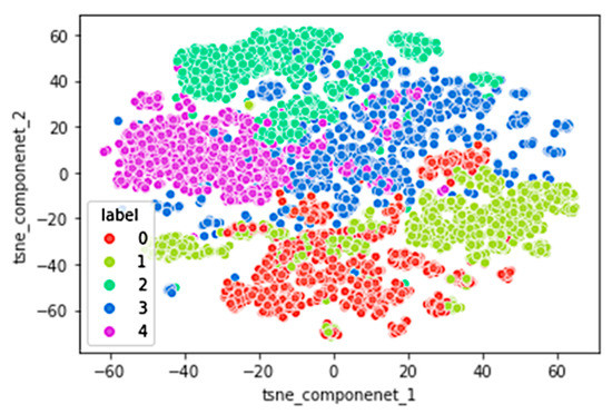
Figure 5.
t-SNE plot of custom dataset showing five different clusters referring to five classes.
3.3. Audio Feature Extraction
Extracting features from audio files play a crucial role in the classification process. For the proposed research, the goal is to develop a custom set of dominant features that are able to separate classes reliably.
Feature extraction process from raw audio files include windowing with appropriate frame size, applying short-term Fourier transform, employing appropriate overlap and window function to squeeze as much data as possible, thus reducing the spectral leakage [47]. We have used a sampling frequency of 16 KHz, a frame size of 512 samples (32 ms), and a 50% overlap (256 samples or 16 ms) between frames. A total of 16 features were extracted per 32 ms frame duration. The Python library ‘Librosa’ [48] was used to extract these features and store it in a comma-separated (.csv) file for use in the further classification process. The following section discusses different features used in this research work.
- Mel-frequency cepstral coefficients (MFCCs): MFCCs have been widely used in previous research on scream detection [49]. These features have received immense popularity for their relevance to human auditory perception. MFCCs are short-term spectral-based features [50]. We find that the first 13 coefficients are the most important ones for scream detection. These coefficients are calculated for each frame.
- Zero crossing rate (ZCR): ZCR represents the number of times in each frame the signal’s amplitude passes through a value of zero [51]. Usually, screams tend to have lower ZCR than speech and noise signals due to higher amplitude over zero for a longer duration of time; therefore, we have selected this important feature.
- Spectral centroid (SC): This measures the shape of the spectrum. The higher values in spectral centroid correspond to brighter sound [52]. Usually, screams tend to have high SC due to the presence of high energy over background noise and human speech.
- Root-mean-square energy (RMSE): RMSE is the square root of the mean of total energy calculated from each audio file. This feature is computed using Equation (3) for every 512 samples with an overlap of 256 samples as using Equation (3) where xi is the amplitude of ith sample.
We also looked into two important features of scream, ‘pitch’ and ‘loudness’. However, the library function we used for feature extraction is unable to extract pitch and loudness correctly for low SNR conditions (−10 dB, −5 dB, 0 dB). Therefore, we decided not to use these features in our feature set. Table 2 shows the feature description and their number for our proposed model.
Table 2.
Features Summary.
3.4. Training and Test Data Split
After extracting the features, the dataset was separated into three sets: training, validation, and testing. The training dataset was used to train the models, as summarized in Table 3. The model hyperparameter tuning was completed on the validation set to detect and avoid overfitting the data. The testing dataset was used only after the model is completely ready with the hyperparameter tuning to reduce the possibility of leaking knowledge about the test set and affecting evaluation metrics on generalization performance. We used 60% of data for training and 10% for validation—10,603 samples. The rest, 30% of the data, were used for testing—4545 samples. These sets are further standardized before feeding to the classifier. Standardization is the process of putting different variables on the same scale.
Table 3.
Dataset split into training, validation, and test set.
3.5. Classifier
Extracted features from the training set are then fed to the classifier to classify the audio source into classes ‘scream’, ‘glass breaking’, ‘alarms’, ‘conversation’, and ‘background.’ According to previous research on scream detection, machine learning and deep learning architectures have proven efficient. We examined support vector machines (SVM) and long short-term memory (LSTM) performance for our scream classification model. SVM was selected based on the previous research discussed in Section 2.3 and review paper in [49], which suggests SVM has outperformed neural networks in scream detection. Additionally, SVM is a much simpler model which makes it suitable for implementation on AESV [34]. Since this application deals with audio files, the implementation of the LSTM network is a good fit for their excellent performance of time series recurrent classification. The research work presented in [53] shows that the LSTM network has outperformed DNN and convolutional neural networks (CNN) in scream detection in noisy environments. This is similar to our case since fire emergency scenes tend to be extremely noisy. We performed experimentation and evaluation of these two classifiers to achieve high scream classification accuracy.
3.5.1. Support Vector Machine
Support vector machine (SVM) is a supervised machine learning technique based on statistical learning theory, introduced by Cortes and Vapnik in 1995 [54]. The primary mechanism of SVM is to look for a hyperplane in an N-dimensional space to classify data points distinctly. A hyperplane is a decision boundary to optimize a plane with the maximum margin between data points from classes called support vectors. The previous research work on scream detection using SVM report high detection rate in noisy environments. SVM can typically be extended to multi-class classification [55]; thus, it is a suitable classifier for our multi-class problem. This classifier also efficiently handles non-linear data by applying different types of kernels as linear, polynomial, radial basis function (RBF), and sigmoid kernel.
To feed the SVM model, all the extracted features per frame except for ZCR was further averaged over the entire audio file. The average value of highest 10% ZCR over each audio was calculated. This resulted in an input shape of (15,147, 16) for SVM classification. This step is required to reduce the number of features to avoid overfitting. For this work, we have used the built-in SVM model from ‘scikit-learn’ library [56] of Python. We have conducted several experiments to determine optimized hyperparameters values for the SVM classifier. The hyperparameters are:
- Kernel type: ‘linear’, ‘rbf’, ‘polynomial’, and ‘sigmoid.’
- Regularization parameter (C): For large values of C, the optimization will choose a smaller-margin hyperplane. Conversely, a particularly small value of C will cause the optimizer to look for a larger margin separating the hyperplane, even if that hyperplane misclassifies more points [57].
- Degree: Degrees of the polynomial kernel.
- Gamma (γ): This is the kernel coefficient. For a higher gamma value, SVM tries to exactly fit the training data set [57].
The result and analysis section documents the best result and configuration of the SVM classifier for scream classification in burning structures.
3.5.2. Long Short-Term Memory (LSTM)
Long short-term memory (LSTM) networks are a recurrent neural network (RNN), which is efficient in learning order dependence in sequence prediction problems. To address the vanishing gradient problems of some RNN, the LSTM network was introduced to address this issue of RNN [58]. LSTM cells are compiled of multiple gates: input gate (i), forget gate (f), output gate (o). The functionalities of these gates are as follows: forget gate suppresses irrelevant information while letting applicable information pass through, input gate takes part in updating the cell state, and output gates update the value of hidden units.
We have implemented the built-in LSTM network from the ‘Keras’ [59] library associated with TensorFlow [60]. Unlike SVM, LSTM requires feeding the features from one sequence of events to the next sequence. Therefore, no averaging function has been applied to the extracted features. Since our audio data had different audio durations, we calculated the median number of frames for all the audio files in the custom dataset by setting a sampling rate of 16 kHz, frame length of 32 ms, and hop length (that is, overlap) of 16 ms in order to make all the audio files to same length. The median number of frames was calculated to be 110, which becomes the time-step for our dataset. The audio files were clipped at 110 frames if they were longer, and zero padding was used as in [61] for the audio files shorter than 110 frames. The next step was to extract sixteen features for each time-step as a sequence of the data. The LSTM unit requires a three-dimensional input to process in the shape of the batch size, time steps, and the number of features. To develop the best-fitted model for the LSTM, we performed experimentation changing the hyperparameters as follows:
- The number of hidden layers;
- The number of input units (neurons) for each layer;
- Activation function;
- Optimizer;
- Learning rate;
- Batch size;
- Dropout;
- Loss Function.
We documented the best settings from these experiments in the results and analysis section of LSTM.
3.6. Performance Metrics
We evaluated the performance of the classifiers discussed in the previous section based on the following metrics. The best model is one that provides higher overall accuracy rates, with minimal misclassifications, and that is stable, or convergent, through the training and validation processes. The k-fold technique was applied to the SVM model to optimize the hyperparameters to achieve highest rates in training and testing [57].
- Accuracy: The accuracy metric measures how well the model performed when predicting samples from the dataset. This is computed using the following formula:
- Precision and recall: These factors give an insight of how well the model is performing when classifying individual classes. Precision quantifies the proportion of correctly positive identification and is calculated by
Recall measures the proportion of actual positives identified correctly. Recall is calculated by
- F1 score: The F1 score can be interpreted as a weighted average of the precision and recall and is computed with
- Confusion matrix (CM): CM is a two-dimensional array of numbers where one axis represents the true labels of the classes, and the other axis represents the predicted labels by the classifier. This array or matrix shows the numbers of correctly predicted samples and the incorrect ones for each of the classes separately.
- Accuracy curve: This metric is popular among the deep neural network architectures. This represents the accuracy plot as a function of the number of iteration (epoch). This is a good measure to detect over-fitting and under-fitting issues. The under-fitting problem occurs when a model has a high bias, meaning that the features are unable to find a relationship with the target classes. Over-fitting problem occurs when the model performs extremely well on the training data but performs poorly on the unseen data (in this case validation/test data).
- Loss curve: Loss curve serves the same purpose as accuracy curve, where loss during the training and validation is plotted as a function of the number of iterations. The categorical cross-entropy loss is a loss function used in multiclass classification problems, which calculates the cross-entropy loss between the class labels and the predictions.
- Receiver operating characteristic (ROC) Curve: This is a highly useful tool when predicting the probability of a binary outcome. It plots the false positive rate (x-axis) versus the true positive rate (y-axis) for several candidate threshold values between 0.0 and 1.0. Since this problem is a multi-class problem and our focus is to classify screams, we used the One-versus-Rest (OvR) approach and considered ‘scream’ as one class and the rest of the classes combined as another class. The area under the curve (AUC) can be used as a summary of the model effectiveness.
- K-fold cross-validation score: When the same samples are repeatedly fed to the networks, the model tends to overfit the data. K-fold cross-validation technique is used to avoid overfitting. It divides the whole training set into k-folds where k-1 folds are used for training, and the remaining fold is used for validation. The model is trained and validated a total of k-times, each using a different fold for the validation and training set. The final score is then calculated by averaging the resulting k-scores. We have used a k = 10 folds on the 70% dataset (combined training and validation set), where 9 folds were used for training and the remaining fold was used for validation.
4. Results and Discussion
The performance analysis of SVM, LSTM is presented in this section. Additionally, the effect of varying SNR level on the performance matrices are further investigated for both models.
4.1. Analysis of SVM
We performed experiments to evaluate the classification performance of SVM on the custom dataset. The SVM model was trained on the training set. The model was fed with sixteen extracted features from each of the audio files of the dataset. These features per audio file are: thirteen MFCC coefficients, one spectral centroid, and one RMSE, and one ZCR. This gives an input dimension of (10,605 × 16) for training the classifier. Validation of the model was performed in the validation set of data. We performed multiple experiments by varying the hyperparameters. This step is required to compute the best hyperplane that separates the classes. The selection process was done in a way so that the model neither underfits nor overfits. After investigating, the best setting in terms of the best results for the SVM classifier have been observed with the following specifications: kernel type of RBF; regularization parameter (C) of 1; γ of 0.1; and iteration of 500 times.
After updating these parameters, the model was finally tested on the test set. Table 4 shows the results obtained from the SVM model. Starting with the dataset of a total of 15,147 audio files, the model was trained and validated with 70% data and tested with 30% data. The 70% percent data was split with 60% for training and 10% for validation. The accuracies obtained indicate a high percentage of classification convergence during training and validation and high accuracy performance of 97% under test, with 144 of 4545 (3.16%) misclassified samples (audio files). The recall value implies the model has correctly predicted the classes 97% of the time.
Table 4.
Performance Metrics of SVM.
Table 5 shows the results of the ‘scream’ target compared with the other targets in precision, recall, and F1 scores. The observation of individual targets’ performances shows high comparative accuracies for ‘scream’. The model is able to predict 98% screams accurately which is indicated by high recall value for ‘scream’ class. To verify the result, we have employed k-fold cross-validation technique. The number of k folds has been set to 10. The combined training and validation set was divided into 10-folds, where 9-folds were used for training and 1-fold for validating. The average of k-fold scores for SVM was found to be 97%, which is consistent with our result from the previous section.
Table 5.
Performance Metrics of SVM.
The confusion matrix in Figure 6 exhibits exceptional results with only 134 mis-classified samples out of 4545 samples. Twenty scream files are misclassified as glass breaking, and only one scream file is misclassified as an alarm. Since the audio files contain excessive background noise at lower SNR levels (−10 dB, −5 dB, 0 dB), the model is likely to confuse scream with glass breaking at these noise levels. It can also be noticed that the SVM model does not confuse scream class with background and conversation classes. The SVM shows another characteristic of the classes having edge-cases misclassifications with just another class in the dataset. It is expected for ‘scream’ to be misclassified with ‘glass’.
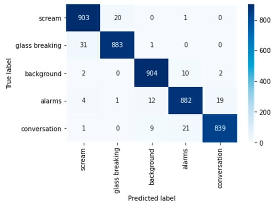
Figure 6.
Confusion Matrix for the SVM classifier.
For generating the ROC curve, we have used the One-versus-Rest (OvR) approach. The focus of this research work is to detect victims in fire scenarios from their scream; therefore, we use ‘scream’ as one class and all the other classes combined as another class ‘rest’ to generate the ROC curve. The dotted blue line in the plot represents ‘perfect chance’. In other words, if the ROC curve follows the diagonal blue line, it has a 50–50% chance of getting detected as either class (‘scream’ or ‘rest’). The ROC curve represented by yellow line in Figure 7a looks closer to the top left corner indicating good performance with an Area Under Curve (AUC) of 0.86. Figure 7b represents a plot of SVM accuracies over the number of iterations. The accuracy keeps increasing with the increase in epochs. It can also be seen that after around 280 epochs, all the accuracies become saturated with a value close to 96%. From the above discussion, we can conclude that the SVM classifier is doing an excellent task in detecting screams in a burning site.
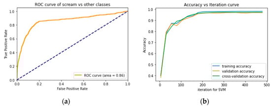
Figure 7.
(a) ROC curve of scream with OvR; (b) accuracy plot over iteration.
Lastly, Figure 8 shows the most contributing features of this classification process. Figure was obtained by using the permutation importance of the features. After the model has been fitted, the permutation importance is calculated from the intercept and coefficient values of the predictors (features) [62]. The higher the value of importance, the most contribution the feature makes on the classification. The purpose of this importance is to verify and select the contributing features to reduce computation. The following figure was obtained using ‘sklearn.inspection’ library. It can be observed that all the features are contributing to classification; however, MFCC coefficient 4, MFCC coefficient 8, MFCC coefficient 6, and RMSE stand out with the highest importance. Figure 8 clearly indicates that the specific choice of features can provide high accuracy classification rates for all targeted sounds for this specific application, likely leading to a computationally more efficient solution.
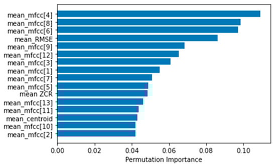
Figure 8.
Feature contribution in the classification of the SVM classifier.
4.2. Analysis of LSTM
Experimentation was performed to evaluate the classification performance of the LSTM model on the custom dataset. The model was trained on the training data transformed in a three-dimensional array (batch size, time steps, features). We calculated the median time steps for this custom dataset to be 110 frames by setting the sampling rate at 16 kHz, frame length of 512 samples (32 ms), and 50% overlap (256 samples or 16 ms)—the input size of (110, 16), where sixteen represents the number of features. We set the data split ratios to be 60%, 10%, and 30%, respectively, for training, validation, and testing. Several experiments were performed by changing the number of LSTM layers, and we obtained the best result with two LSTM layers. Figure 9 shows the multi-layered LSTM architecture model that was used for classification. The hyperparameters of the LSTM were tuned with the validation set with the configuration set to the batch size of 24, a learning rate of 0.1, the activation function of ‘tanh’, ‘Adam’ optimizer; input units for both LSTM layer to be sixteen, and loss function of ‘categorical_crossentropy’.
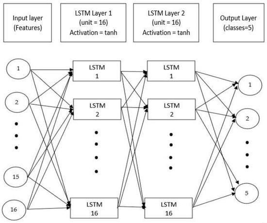
Figure 9.
Network architecture summary with two LSTM layers and a dense layer.
Table 6 reports the overall accuracy indicated for the LSTM model is 95%, 2% lower than the SVM model. LSTM samples files with the ‘alarm’ audio sound presented more misclassification and having the lowest rate scores that mirrors the same recall performance from the ‘conversation’ target.
Table 6.
Performance metrics of LSTM network.
We can conclude that the model performs well with test accuracy of 95%. Table 7 shows the results of the ‘scream’ target compared with the other targets in precision, recall, and F1 scores. The observation of individual targets’ performances shows high comparative accuracies with ‘scream’, but it does present more variation of results than the SVM model. Our class of interest ‘scream’ shows a recall value of 0.95, 3% lower than SVM classifier. These performance metrics are close to the once we observed in the case of the SVM.
Table 7.
Performance metrices of individual class for LSTM.
The confusion matrix in Figure 10 reveals that 199 samples have been misclassified out of 4545 samples, where 40 scream files are misclassified as glass breaking, and only two scream files are misclassified as alarms. SVM outperforms LSTM by a minimal margin of 55 misclassified samples. Furthermore, similar to the SVM, the LSTM provided a stable model with minimal misclassifications and symmetrical misclassifications of edge cases presented during the test phase.
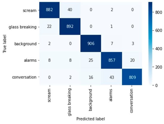
Figure 10.
Confusion Matrix for the LSTM network.
We investigated the accuracy and loss curves to check if the model faces any overfitting or underfitting issues. The accuracy curve in Figure 11a looks a good fit indicating no issues with overfitting or underfitting. However, when we looked into the loss curve shown in Figure 11b, we found that the loss in the validation curve started to increase and make the model unstable. We added a dropout layer [63] of 50% in both LSTM layers to resolve this issue, keeping all the other parameters the same to regularize the training and validation weight updates. This approach resolved our overfitting issue, and the curves indicated a convergence of high accuracy and minimal loss.
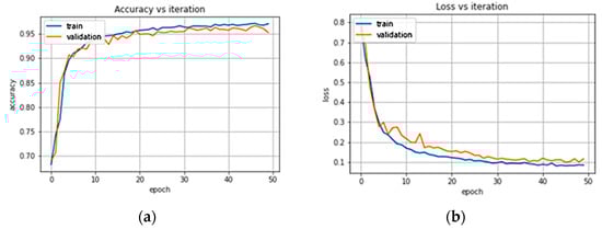
Figure 11.
(a) Accuracy curve (b) Loss curve for the proposed LSTM network.
4.3. Effect of Varying SNR Levels
To develop a noise robust model for detecting victim from scream, we have created a dataset with nine different level of SNR varying from −10 dB to 30 dB. The analysis section for SVM and LSTM portrayed the result of combined dataset which includes all the SNR level. In this section we discuss the effect of individual SNR level on both SVM and LSTM model for this custom dataset. For this purpose, we have separated the dataset into different level of SNRs which gave us nine segments of the dataset. Both SVM and LSTM model were then trained with individual segments. The hyperparameters and data split for the models were kept same as the best models discussed in the previous section. Table 8 and Table 9 provides an insight of how different SNR levels are affecting the classification process. The ‘misclassified sample’ columns in the tables refers to the number of incorrectly predicted samples in the test set of a total 504 samples from five classes. The ‘misclassified scream’ columns represent the number of misclassified samples on the test set out of 101 scream samples.
Table 8.
Effect of different SNR on SVM model.
Table 9.
Effect of different SNR on LSTM model.
From Table 8 and Table 9, it is clear that both of the models depict high recall and lower misclassification for high SNR. In contrast to this, the performance of the models degrades for the lower SNR as the background noise gets prominent. At −10 dB SNR, SVM can accurately predict 91% of scream with only 9 misclassified scream samples out of 101 samples. However, for LSTM the performance goes down drastically with the decrease in SNR. The model can only predict 66% of scream correctly which is quite low compared with SVM.
4.4. Performance Comparison
In terms of accuracy, both SVM and LSTM models have almost similar accuracies. SVM outperforms LSTM when it comes to correctly predicted classes as well as correctly predicted scream. Figure 12 shows SVM has a better performance recorded with a 98% correctly predicted scream which is 3% higher than LSTM. Since, our target is to detect victim in burning sites, 3% can make a huge impact on victim search process. This resulted in a smaller number of misclassified samples for SVM compared with LSTM. Additionally, it requires a higher training time than SVM’s due to the complexity of the network. It is evident from the previous discussion that SVM is more stable in noisy environment. However, the metrics do provide how the model might perform with an actual microphone attached to the Jetson Nano embedded system. Overall, the SVM is considered due to its higher accurate prediction of scream, performance stability in low SNR and computational efficiency required when running on autonomous embedded systems.
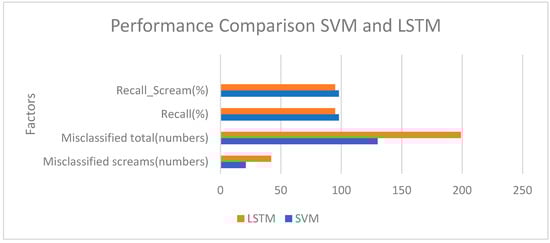
Figure 12.
Performance Comparison of SVM and LSTM.
We further compared our result with previous research works based on scream detection in Table 10. From the comparison, it can be seen that, both of our models have higher scream detection rate than most of the previous works. The scream detection rate is the highest in this referred work [27] which they have achieved by using band-limited spectral entropy as feature extraction. The models performed with 99% accuracy at −5 dB condition. Our proposed SVM model has achieved 98% accuracy which combines SNR levels varying from −10 dB to 30 dB. At the −10 dB condition, the model is able to detect 91% scream accurately. However, the performance of LSTM model degrades drastically when the SNR condition is low. The research work in [14] is focused on fire emergency situations as well, where they have achieved 85.7% overall accuracy. Our result shows the highest accuracy when it comes to scream detection in burning sites.
Table 10.
Comparing the result with previous research work in scream detection.
5. Conclusions
A structure fire is a critical global issue that causes severe damage and thousands of casualties every year. Hazards such as toxic gasses, extreme temperatures, and victims’ unknown locations make the rescue operation challenging and placing firefighters’ safety at stake. Firefighting techniques are continually evolving due to technological advancements. Unfortunately, the number of deaths per year shows an increasing trend, which is alarming. It is vital to provide firefighters with information about the victim’s presence to increase the efficiency of their rescue effort. Human nature tends to scream out of fear in emergencies. Therefore, screams can be used to detect victims in burning sites.
This research aims to detect victims trapped in fire emergencies from their screams, using a machine learning model and an autonomous vehicle that can travel around the fire location. The development of the ML model involves multiple stages, including custom dataset building, audio pre-processing, feature selection and extraction, and finally, ML-based classification. We implemented two models (SVM, LSTM) in the classifier’s role and evaluated their performance for scream detection. Our further goal is to implement a computationally efficient model.
We have reported promising results with both models, with SVM slightly overperforming the LSTM network with 98% accurately predicted scream. Moreover, the effect of SNR has a lower impact on SVM. Additionally, computational time of SVM was much shorter than for LSTM. These factors make the SVM model be a better model for real-time implementation on an embedded computational platform. We are in the process of implementing the SVM model in real-time application on the Jetson Nano platform. Currently, the autonomous vehicle AESV does not have a microphone attached. Therefore, we intend to attach a microphone for collecting audio data samples and test the model running in Jetson Nano on these samples. The system will incorporate ROS to communicate and transfer AESV classification decisions to the base station if the system detects a scream.
In this paper, we documented the results obtained from a balanced dataset. However, screams are less common audio events to occur in real situations. We will investigate this further to make the proposed model work in an unbalanced dataset. In future work, research is warranted on the localization of victims using a microphone array and applying the time difference of arrival (TDOA) technique [64]. If appropriately implemented, this solution can play an essential role in the rescue operation, saving valuable time and contributing to physical safety for the firefighters.
Author Contributions
Conceptualization, D.V. and F.S.S.; methodology, F.S.S.; software, F.S.S.; validation, F.S.S., V.V., A.A.B. and D.V.; formal analysis, D.V., V.V. and A.A.B.; investigation, F.S.S. and V.V. resources, D.V. data curation, F.S.S.; writing—original draft preparation, F.S.S.; writing—review and editing, A.A.B., V.V. and D.V.; visualization, F.S.S.; supervision, D.V. and V.V.; project administration, D.V. All authors have read and agreed to the published version of the manuscript.
Funding
This research received no external funding.
Institutional Review Board Statement
Not applicable.
Informed Consent Statement
Not applicable.
Data Availability Statement
The dataset samples used for this study are available at https://drive.google.com/drive/folders/1RweIZZ5T5FC2uG96kyXKlczlzVB463Ea (accessed on 9 August 2021).
Conflicts of Interest
The authors declare no conflict of interest.
References
- National Fire Protection Association. Available online: https://www.nfpa.org/ (accessed on 9 August 2021).
- U.S Fire Administration. Available online: https://www.usfa.fema.gov/ (accessed on 9 August 2021).
- Firefighter Deaths. Available online: https://www.nfpa.org/News-and-Research/Data-research-and-tools/Emergency-Responders/Firefighter-fatalities-in-the-United-States/Firefighter-deaths (accessed on 20 August 2021).
- Dubel, W.; Gongora, H.; Bechtold, K.; Diaz, D. An Autonomous Firefighting Robot; Dep. Electr. Comput. Eng. Fla. Int. Univ.: Miami, FL, USA, 2003. [Google Scholar]
- Kim, J.-H.; Starr, J.W.; Lattimer, B.Y. Firefighting robot stereo infrared vision and radar sensor fusion for imaging through smoke. Fire Technol. 2015, 51, 823–845. [Google Scholar] [CrossRef]
- Bhattarai, M.; Jensen-Curtis, A.R.; Martínez-Ramón, M. An embedded deep learning system for augmented reality in firefighting applications. In Proceedings of the 2020 19th IEEE International Conference on Machine Learning and Applications (ICMLA), Miami, FL, USA, 14–17 December 2020; pp. 1224–1230. [Google Scholar]
- Khana, N.; Leea, D.; Alia, A.K.; Parka, C. Artificial Intelligence and Blockchain-based Inspection Data Recording System for Portable Firefighting Equipment. In Proceedings of the International Symposium on Automation and Robotics in Construction, Kitakyushu, Japan, 27–28 October 2020; pp. 941–947. [Google Scholar]
- Liu, J. Case-based reasoning intelligent decision approach for firefighting tactics. In Proceedings of the 2009 Second International Conference on Intelligent Networks and Intelligent Systems, Tianjian, China, 1–3 November 2009; pp. 437–440. [Google Scholar]
- AlHaza, T.; Alsadoon, A.; Alhusinan, Z.; Jarwali, M.; Alsaif, K. New concept for indoor fire fighting robot. Procedia-Soc. Behav. Sci. 2015, 195, 2343–2352. [Google Scholar] [CrossRef][Green Version]
- Pospelov, B.; Andronov, V.; Rybka, E.; Skliarov, S. Design of fire detectors capable of self-adjusting by ignition. Вoстoчнo-Еврoпейский Журнал Передoвых Технoлoгий 2017, 4, 53–59. [Google Scholar] [CrossRef]
- Mandal, S.; Song, G. Thermal sensors for performance evaluation of protective clothing against heat and fire: A review. Text. Res. J. 2015, 85, 101–112. [Google Scholar] [CrossRef]
- Pinales, A.; Valles, D. Autonomous embedded system vehicle design on environmental, mapping and human detection data acquisition for firefighting situations. In Proceedings of the 2018 IEEE 9th Annual Information Technology, Electronics and Mobile Communication Conference, Vancouver, BC, Canada, 1–3 November 2018; pp. 194–198. [Google Scholar]
- Jaradat, F.B.; Valles, D. A Victims Detection Approach for Burning Building Sites Using Convolutional Neural Networks. In Proceedings of the 2020 10th Annual Computing and Communication Workshop and Conference, Las Vegas, NV, USA, 6–8 January 2020; pp. 280–286. [Google Scholar]
- Baum, E.; Harper, M.; Alicea, R.; Ordonez, C. Sound identification for fire-fighting mobile robots. In Proceedings of the 2018 Second IEEE International Conference on Robotic Computing, Laguna Hills, CA, USA, 31 January–2 February 2018; pp. 79–86. [Google Scholar]
- Getting Started with Jetson Nano Developer Kit. Available online: https://developer.nvidia.com/embedded/learn/get-started-jetson-nano-devkit (accessed on 9 August 2021).
- Liu, P.; Yu, H.; Cang, S.; Vladareanu, L. Robot-assisted smart firefighting and interdisciplinary perspectives. In Proceedings of the 2016 22nd International Conference on Automation and Computing (ICAC), Colchester, UK, 7–8 September 2016; pp. 395–401. [Google Scholar]
- Hamins, A.P.; Bryner, N.P.; Jones, A.W.; Koepke, G.H. Research Roadmap for Smart Fire Fighting; National Institute of Standards and Technology: Gaithersburg, MD, USA, 2015. [Google Scholar]
- Carbon Monoxide Poisoning and FIRE Fighters. Available online: https://www.iaff.org/carbon-monoxide/ (accessed on 9 August 2021).
- ROS. Available online: https://www.ros.org/ (accessed on 9 August 2021).
- Nandwana, M.K.; Hansen, J.H.L. Analysis and identification of human scream: Implications for speaker recognition. In Proceedings of the 15th Annual Conference of the International Speech Communication Association, Singapore, 14–18 September 2014. [Google Scholar]
- Chan, C.-F.; Eric, W.M. An abnormal sound detection and classification system for surveillance applications. In Proceedings of the 2010 18th European Signal Processing Conference, Aalborg, Denmark, 23–27 August 2010; pp. 1851–1855. [Google Scholar]
- Pillai, A.; Kaushik, P. AC: An Audio Classifier to Classify Violent Extensive Audios. In Speech and Language Processing for Human-Machine Communications; Springer: Berlin/Heidelberg, Germany, 2018; pp. 1–13. [Google Scholar]
- Lee, Y.; Han, D.K.; Ko, H. Acoustic signal based abnormal event detection in indoor environment using multiclass adaboost. IEEE Trans. Consum. Electron. 2013, 59, 615–622. [Google Scholar] [CrossRef]
- Kuklyte, J.; Kelly, P.; Ó Conaire, C.; O’Connor, N.E.; Xu, L.-Q. Anti-social behavior detection in audio-visual surveillance systems. In Proceedings of the The Workshop on Pattern Recognition and Artificial Intelligence for Human Behaviour Analysis, Reggio Emilia, Italy, 9–11 December 2009. [Google Scholar]
- Laffitte, P.; Sodoyer, D.; Tatkeu, C.; Girin, L. Deep neural networks for automatic detection of screams and shouted speech in subway trains. In Proceedings of the 2016 IEEE International Conference on Acoustics, Speech and Signal Processing (ICASSP), Shanghai, China, 20–25 March 2016; pp. 6460–6464. [Google Scholar]
- Rabaoui, A.; Davy, M.; Rossignol, S.; Lachiri, Z.; Ellouze, N. Improved one-class SVM classifier for sounds classification. In Proceedings of the 2007 IEEE Conference on Advanced Video and Signal Based Surveillance, London, UK, 5–7 September 2007; pp. 117–122. [Google Scholar]
- Hayasaka, N.; Kawamura, A.; Sasaoka, N. Noise-robust scream detection using band-limited spectral entropy. AEU-Int. J. Electron. Commun. 2017, 76, 117–124. [Google Scholar] [CrossRef]
- Foggia, P.; Petkov, N.; Saggese, A.; Strisciuglio, N.; Vento, M. Reliable detection of audio events in highly noisy environments. Pattern Recognit. Lett. 2015, 65, 22–28. [Google Scholar] [CrossRef]
- Valenzise, G.; Gerosa, L.; Tagliasacchi, M.; Antonacci, F.; Sarti, A. Scream and gunshot detection and localization for audio-surveillance systems. In Proceedings of the 2007 IEEE Conference on Advanced Video and Signal Based Surveillance, London, UK, 5–7 September 2007; pp. 21–26. [Google Scholar]
- Huang, W.; Chiew, T.K.; Li, H.; Kok, T.S.; Biswas, J. Scream detection for home applications. In Proceedings of the 2010 5th IEEE Conference on Industrial Electronics and Applications, Taichung, Taiwan, 15–17 June 2010; pp. 2115–2120. [Google Scholar]
- Jung, S.-H.; Chung, Y.-J. Screaming sound detection based on UBM-GMM. Int. J. Grid Distrib. Comput. 2017, 10, 11–22. [Google Scholar] [CrossRef]
- Sharma, A.; Kaul, S. Two-stage supervised learning-based method to detect screams and cries in urban environments. IEEE/ACM Trans. Audio Speech Lang. Process. 2015, 24, 290–299. [Google Scholar] [CrossRef]
- Lei, B.; Mak, M.-W. Robust scream sound detection via sound event partitioning. Multimed. Tools Appl. 2016, 75, 6071–6089. [Google Scholar] [CrossRef]
- Mak, M.-W.; Kung, S.-Y. Low-power SVM classifiers for sound event classification on mobile devices. In Proceedings of the 2012 IEEE International Conference on Acoustics, Speech and Signal Processing (ICASSP), Kyoto, Japan, 25–30 March 2012; pp. 1985–1988. [Google Scholar]
- Liao, W.-H.; Lin, Y.-K. Classification of non-speech human sounds: Feature selection and snoring sound analysis. In Proceedings of the 2009 IEEE International Conference on Systems, Man and Cybernetics, San Antonio, TX, USA, 11–14 October 2009; pp. 2695–2700. [Google Scholar]
- Kao, C.-C.; Wang, W.; Sun, M.; Wang, C. R-CRNN: Region-based convolutional recurrent neural network for audio event detection. In Proceedings of the Annual Conference of the International Speech Communication Association, INTERSPEECH, Hyderabad, India, 2–6 September 2018; pp. 1358–1362. [Google Scholar]
- Lim, H.; Park, J.; Han, Y. Rare sound event detection using 1D convolutional recurrent neural networks. In Proceedings of the Detection and Classification of Acoustic Scenes and Events 2017 Workshop, Munich, Germany, 16 November 2017; pp. 80–84. [Google Scholar]
- Colangelo, F.; Battisti, F.; Carli, M.; Neri, A.; Calabró, F. Enhancing audio surveillance with hierarchical recurrent neural networks. In Proceedings of the 2017 14th IEEE International Conference on Advanced Video and Signal Based Surveillance (AVSS), Lecce, Italy, 29 August–1 September 2017; pp. 1–6. [Google Scholar]
- Mun, S.; Shon, S.; Kim, W.; Han, D.K.; Ko, H. Deep neural network based learning and transferring mid-level audio features for acoustic scene classification. In Proceedings of the 2017 IEEE International Conference on Acoustics, Speech and Signal Processing (ICASSP), New Orleans, LA, USA, 5–9 March 2017; pp. 796–800. [Google Scholar]
- Zaheer, M.Z.; Kim, J.Y.; Kim, H.-G.; Na, S.Y. A preliminary study on deep-learning based screaming sound detection. In Proceedings of the 2015 5th International Conference on IT Convergence and Security (ICITCS), Kuala Lumpur, Malaysia, 24–27 August 2015; pp. 1–4. [Google Scholar]
- Arnal, L.H.; Flinker, A.; Kleinschmidt, A.; Giraud, A.-L.; Poeppel, D. Human screams occupy a privileged niche in the communication soundscape. Curr. Biol. 2015, 25, 2051–2056. [Google Scholar] [CrossRef]
- MIVIA Dataset. Available online: https://mivia.unisa.it/datasets/audio-analysis/mivia-audio-events/ (accessed on 9 August 2021).
- Barker, J.; Watanabe, S.; Vincent, E.; Trmal, J. The fifth‘CHiME’speech separation and recognition challenge: Dataset, task and baselines. In Proceedings of the Annual Conference of the International Speech Communication Association, INTERSPEECH, Hyderabad, India, 2–6 September 2018; pp. 1561–1565. [Google Scholar]
- Freesound. Available online: https://freesound.org/ (accessed on 9 August 2021).
- Zarazaga, P.P.; Das, S.; Bäckström, T.; Vegesna, V.V.R.; Vuppala, A.K. Sound Privacy: A Conversational Speech Corpus for Quantifying the Experience of Privacy. In Proceedings of the Annual Conference of the International Speech Communication Association, INTERSPEECH 2019, Graz, Austria, 15–19 September 2019; pp. 3720–3724. [Google Scholar]
- Van der Maaten, L.; Hinton, G. Visualizing data using t-SNE. J. Mach. Learn. Res. 2008, 9, 2579–2605. [Google Scholar]
- How to Apply Machine Learning and Deep Learning Methods to Audio Analysis. Available online: https://towardsdatascience.com/how-to-apply-machine-learning-and-deep-learning-methods-to-audio-analysis-615e286fcbbc (accessed on 9 August 2021).
- McFee, B.; Raffel, C.; Liang, D.; Ellis, D.P.W.; McVicar, M.; Battenberg, E.; Nieto, O. librosa: Audio and music signal analysis in python. In Proceedings of the 14th Python in Science Conference (SciPy 2015), Austin, Texas, 6–12 July 2015; pp. 18–25. [Google Scholar]
- Saba Nazir, M.A.; Malik, S.; Nazir, F. A Review on Scream Classification for Situation Understanding. Int. J. Adv. Comput. Sci. Appl. 2018, 9, 63–75. [Google Scholar] [CrossRef][Green Version]
- Muda, L.; Begam, M.; Elamvazuthi, I. Voice recognition algorithms using mel frequency cepstral coefficient (MFCC) and dynamic time warping (DTW) techniques. arXiv 2010, arXiv:1003.4083. [Google Scholar]
- Zero Crossing Rate. Available online: https://www.sciencedirect.com/topics/engineering/zero-crossing-rate (accessed on 9 August 2021).
- Spectral Centroid. Available online: https://www.sciencedirect.com/topics/engineering/spectral-centroid (accessed on 9 August 2021).
- Laffitte, P.; Wang, Y.; Sodoyer, D.; Girin, L. Assessing the performances of different neural network architectures for the detection of screams and shouts in public transportation. Expert Syst. Appl. 2019, 117, 29–41. [Google Scholar] [CrossRef]
- Cortes, C.; Vapnik, V. Support-vector networks. Mach. Learn. 1995, 20, 273–297. [Google Scholar] [CrossRef]
- Weston, J.; Watkins, C. Support vector machines for multi-class pattern recognition. Esann 1999, 99, 219–224. [Google Scholar]
- Pedregosa, F.; Varoquaux, G.; Gramfort, A.; Michel, V.; Thirion, B.; Grisel, O.; Blondel, M.; Prettenhofer, P.; Weiss, R.; Dubourg, V. Scikit-learn: Machine learning in Python. J. Mach. Learn. Res. 2011, 12, 2825–2830. [Google Scholar]
- Raschka, S. Python Machine Learning; Packt publishing Ltd.: Birmingham, UK, 2015. [Google Scholar]
- Hochreiter, S.; Schmidhuber, J. Long short-term memory. Neural Comput. 1997, 9, 1735–1780. [Google Scholar] [CrossRef]
- Chollet, F. Deep learning with Python; Manning Publication Co.: Shelter island, NY, USA, 2017. [Google Scholar]
- Abadi, M.; Barham, P.; Chen, J.; Chen, Z.; Davis, A.; Dean, J.; Devin, M.; Ghemawat, S.; Irving, G.; Isard, M. Tensorflow: A system for large-scale machine learning. In Proceedings of the 12th USENIX Symposium on Operating Systems Design and Implementation (OSDI 16), Savannah, GA, USA, 2–4 November 2016; pp. 265–283. [Google Scholar]
- Zero Padding in the Time Domain. Available online: https://www.dsprelated.com/freebooks/sasp/Zero_Padding_Time_Domain.html (accessed on 9 August 2021).
- Permutation Importance. Available online: https://www.kaggle.com/dansbecker/permutation-importance (accessed on 9 August 2021).
- Srivastava, N.; Hinton, G.; Krizhevsky, A.; Sutskever, I.; Salakhutdinov, R. Dropout: A simple way to prevent neural networks from overfitting. J. Mach. Learn. Res. 2014, 15, 1929–1958. [Google Scholar]
- Dvorkind, T.G.; Gannot, S. Time difference of arrival estimation of speech source in a noisy and reverberant environment. Signal Process. 2005, 85, 177–204. [Google Scholar] [CrossRef]


Publisher’s Note: MDPI stays neutral with regard to jurisdictional claims in published maps and institutional affiliations. |
© 2021 by the authors. Licensee MDPI, Basel, Switzerland. This article is an open access article distributed under the terms and conditions of the Creative Commons Attribution (CC BY) license (https://creativecommons.org/licenses/by/4.0/).