A Method of Enhancing Rapidly-Exploring Random Tree Robot Path Planning Using Midpoint Interpolation

Abstract

It is difficult to guarantee optimality using the sampling-based rapidly-exploring random tree (RRT) method. To solve the problem, this paper proposes the post triangular processing of the midpoint interpolation method to minimize the planning time and shorten the path length of the sampling-based algorithm. The proposed method makes a path that is closer to the optimal path and somewhat solves the sharp path problem through the interpolation process. Experiments were conducted to verify the performance of the proposed method. Applying the method proposed in this paper to the RRT algorithm increases the efficiency of optimization by minimizing the planning time.

1. Introduction

Recent path planning research for the robot has encompassed a wide range of topics [1,2]. Path planning is an important capability for autonomous mobile robots. A robot must be able to identify a path from its current position to its destination in order to move successfully. A mobile robot must be able to discover an optimal or sub-optimal collision-free path in the environment from the starting position to the destination [3].

Path planning is the formulation of a route for a mobile robot to proceed from a starting point to a destination point in Euclidean space as efficiently as possible while avoiding both static and dynamic obstacles and maintaining optimality, clearance, and completeness [4]. An optimal path is one with the ideal path length, a clear path is one without obstacles for the mobile robot to collide with, and a complete path is one in which the robot can move from the start point to the destination point without colliding with obstacles.

Furthermore, it is indeed possible for the robot to be able to optimize its path by determining the quickest and safest path to its destination point in order to save time and energy. However, an algorithm that generates the optimal path increases the computation, and an algorithm that quickly generates a path does not guarantee the optimal path [5].

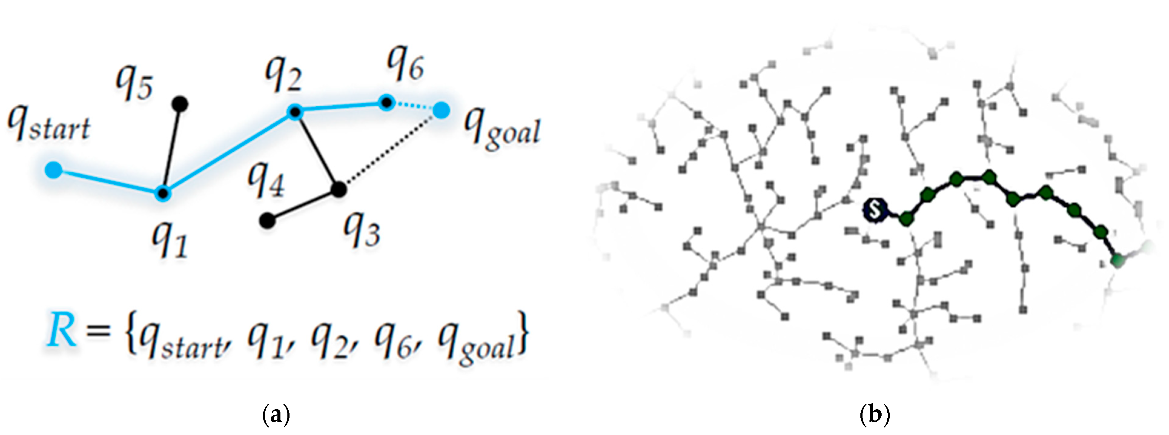
It is difficult to ensure optimality with the sampling-based rapidly-exploring random tree (RRT) algorithm [6]. As shown in Figure 1a, the RRT algorithm is a path planning algorithm that involves repeatedly adding a randomly sampled position as a child node in a tree with the starting point as the root node until the destination point is reached. The tree extends out in the shape of a stochastic fractal, as shown in Figure 1b, and has an algorithm used to locate the destination point.

Figure 1. Overview of the rapidly-exploring random tree (RRT) algorithm: (a) planned path R from starting point q_start through waypoints q₁, q₂, q₆ to destination q_goal (q_i is a point on the path); (b) process of finding destination point by stochastic fractal shape from the root node (S) as a starting point.

The RRT algorithm and other sampling-based algorithms [7,8] offer the benefit of planning a path in a shorter time with less computing than traditional path planning algorithms like the visibility graph- [9], cell decomposition- [10], and potential field-based algorithms [11]. On the other hand, it does not ensure optimality and has the drawback of having probabilistically assured completeness. The latter is also known as probabilistic completeness [12], which implies that completeness is assured when the number of random samples is infinite but not always when the number of random samples is limited. The goal of this research is to enhance the RRT algorithm, which ensures completeness and performs better than the related algorithms.

To solve these problems, the main idea of the proposed post triangular processing of midpoint interpolation method is effective in path planning algorithms that do not guarantee optimality, such as the RRT algorithm that has a locally piecewise linear shape and can be used as a post-processing method after a path has been planned using one of these algorithms. It may also be used for different route planning methods since it is a post-processing technique that has no impact on calculation time.

The sampling-based path planning algorithm’s primary strength is the fast planning speed based on the small amount of computation compared to the traditional path planning algorithms [7].

Performance verification using simulation in various environments and mathematical modeling were used to validate the performance of the proposed method in this paper. The case in which the proposed algorithm is applied to the sampling-based path planning method and the case in which it is not applied are compared through simulation. Here, the planning time and path length of the first complete path to reach a destination point from a starting point are evaluated.

This paper is organized as follows: Section 2 reviews some related works. Section 3 introduces the proposed post triangular processing of the midpoint interpolation method. Various experimental environments are constructed for path planning in Section 4 to examine the effectiveness and improvements of the proposed method. Finally, the conclusions are presented in Section 5.

2. Related Works

In this section, we introduce the previous works about the RRT algorithm in Section 2.1 and the Triangular Rewiring Method for the RRT Algorithm in Section 2.2, respectively.

2.1. RRT

This section shows the pseudocode of the RRT algorithm used in the experiment of this paper that was designed based on [6] in which the RRT algorithm was proposed. In 1998, LaValle proposed the RRT algorithm, which is a representative sampling-based path planning algorithm [6]. It is designed to have many degrees of freedom and is useful for planning a path under non-holonomic constraints.

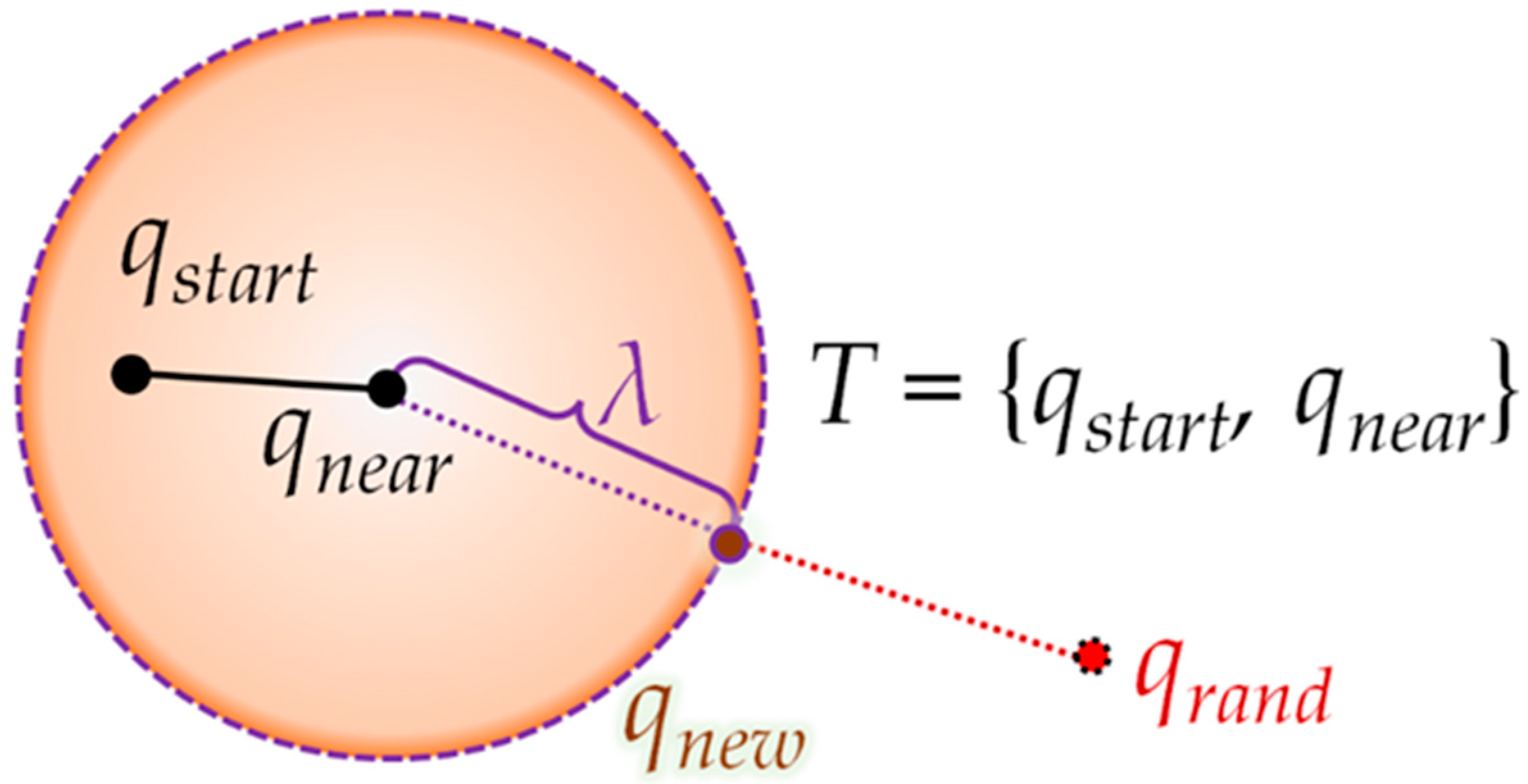
As shown in Figure 2, when a random sample is generated in the configuration space, the node nearest to the position of the random sample is identified among the nodes constituting the tree with the starting point as the root node. A new node is generated at the random sample position and inserted into the tree if the random sample position is nearer than the step length. The process of tree extension is repeated until the destination point is reached. The RRT algorithm implemented for the proposed method and comparison experiment is Algorithm 1.

Algorithm 1 Pseudocode of RRT Algorithm
Input:
qstart ← start point
qgoal ← goal point
λ ← step length
C ← position set of all (measured) boundary points in all (known) obstacles
N ← number of random samples
Output:
R ← result of path R
Initialize:
T ← Null tree<node, edge>
ProcedureRRT
Begin
1	T ← Insert root node<qstart> to T
2	Whilen ← 0 To N Do
3	Generate n-th random sample
4	qrand ← position of n-th random sample
5	qnear ← position of the nearest node in T from qrand
6	If not isInside(qnear, qrand, λ) Then
7	qnew ← intersection point between line segment connecting qrand and qnear,     and circle with radius λ centered at qnear
8	Else qnew ← qrand
9	If not isTrapped(qnew, qnear, C) Then
10	T ← Insert node<qnew> and edge<qnew, qnear> to T
11	If isInside(qnew, qgoal, λ) Then
12	T ← Insert node<qgoal> and edge<qnew, qgoal> to T
13	P ← path from last inserted node{qgoal} to root node{qstart} in T
14	If [length of R] > [length of P] Then  R ← P
15	T ← Delete node<qgoal> and edge<qnew, qgoal> from T
End

Figure 2. Process of the RRT algorithm: When creating the new node q_new at a position separated by step length λ in direction of random sample position (q_rand) based on q_near node (position) closest to random sample position (q_rand) in tree T with starting point q_start as the root node.

In order to overcome the limitations on optimality and convergence time [6], RRT-Connect can find a connected path more quickly by setting the start point and the destination point as the root of a separate tree, and further expanding the two trees alternately [7]. Rapidly-exploring Random Tree Star (RRT*) [13] was developed to overcome the limitation that the path generated from RRT does not guarantee convergence to the optimal path. Informed-RRT* that can find a connected path quickly by enhancing the sampling probability inside the elliptical region with the start point and the destination point as the respective focal points [14]. The RRT*-Connect algorithm combines the advantages of RRT-Connect and RRT* [15]. RRT*-Smart [16], Quick-RRT*[17], and the proposed algorithm in [8] can show closer optimality by finding and connecting linearly connectable ancestor nodes to random samples through triangular inequality in the process of adding random samples.

2.2. Triangular Rewiring Method for the RRT Algorithm

This section shows the principle and pseudocode of the Triangular Rewiring Method for the RRT algorithm.

The triangular rewiring method is used to rewire the component based on the triangular inequality concept [8]. The triangular inequality-based RRT algorithm is a rewiring of the RRT method that is based on the concept of triangular inequality between nodes in path planning; thus, it is closer to the optimum than the RRT.

The triangular rewiring method not only can find a better initial solution but also can converge to a better solution rapidly.

The pseudocode for the triangular rewiring method is shown in Algorithm 2. This iterative process continues until no q_ancestor exists (when no parent node exists for the previous q_ancestor, i.e., when q_ancestor is q_start) or an obstacle exists between q_child and q_ancestor. The method for triangular rewiring is as follows: the node with the position q_parent and the edge connecting the q_child and q_ancestor nodes are deleted. After the edge is deleted, the q_ancestor node is updated with the q_parent node, and the parent node of the q_ancestor is updated with the q_ancestor node. The existing q_parent node is then deleted. Then, the Trapped method is used to check if it collides with an obstacle between the q_child node and the updated q_parent node. Then, in tree T, the last created q_parent is inserted as the parent node of q_child.

Algorithm 2 Pseudocode of Triangular Rewiring Method for RRT Algorithm
Input:
qchild ← Position {qnew/qnewA/qnewB}
qparent ← Position qnear
T ← Tree {Tmerged/Ta/Tb}
C ← Position Set C
Output:
{Tmerged/Ta/Tb} ← Result of T
Begintriangular RewiringProcedure
1	qancestor ← Position of Parent Node of qparent in T
2	If NotisTrapped(qancestor, qchild, C) then
3	T ← Delete Node<qparent>, Edge<qparent, qchild> and Edge<qparent, qancestor> from T
4	qparent ← qancestor
5	qancestor ← Position of Parent Node of qancestor in T
6	While Not qancestor = Null do
7	If Not isTrapped(qancestor, qchild, C) then
8	T ← Delete Node<qparent> and Edge<qparent, qancestor> from T
9	qparent ← qancestor
10	qancestor ← Position of Parent Node of qancestor in T
11	Else
12	Break
13	T ← Insert Edge<qparent, qchild> to T
14	Else
15	T ← Insert Node<qchild> and Edge<qchild, qparent> to T
Endtriangular RewiringProcedure

3. Proposed Post Triangular Processing of the Midpoint Interpolation Method

The proposed post triangular processing of the midpoint interpolation method can be applied to path planning algorithms that do not guarantee optimality, such as the RRT algorithm, and rewiring and midpoint interpolation based on the triangular inequality principle.

The assumptions of the proposed method are as follows:

• The destination point may change gradually over time, but there is only one start point and one destination point for each tree.
• If the mobile robot cannot perform the omnidirectional motion, local planning or kinodynamic planning is performed separately on the path planning result.

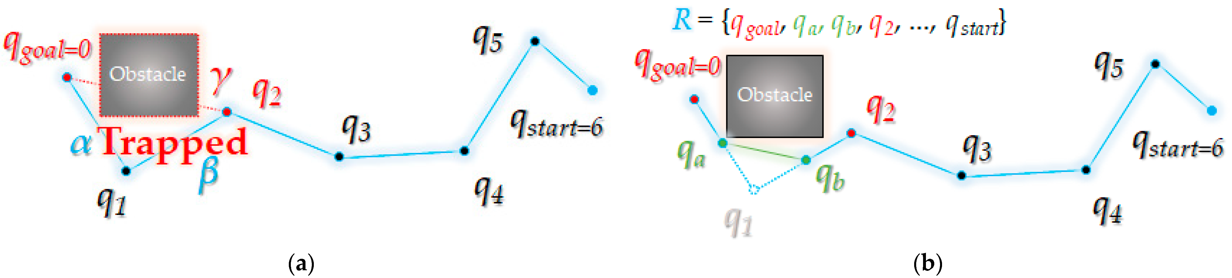
The basic principle is that the node serving as a waypoint in the planned path checks whether an obstacle collides with its own grandparent node, and if it is free from obstacle collision, the grandparent node rewires to the parent node. If it is not free from obstacle collision, as shown in Figure 3, the locally piecewise linear path created between the node, its parent node, and its grandparent node is made a more optimal path through the interpolation process. In this process, a new node is interpolated into the path and deviates from the piecewise linear path, so it has the advantage of being able to somewhat solve the sharp path problem (the problem facing a mobile robot that has kinematic constraints because the slope is not smooth).

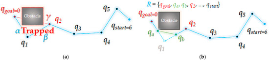
Figure 3. Summary of post triangular processing of the midpoint interpolation method: (a) line segment γ with node q₀ and its grandparent node q₂ in tree R is not free from obstacle collision; (b) Parent node q₁ of q₀ is deleted, and q_a between q₀ and q₁, and q_b between q₁ and q₂ are inserted as waypoints of a new path between q₀ and q₂.

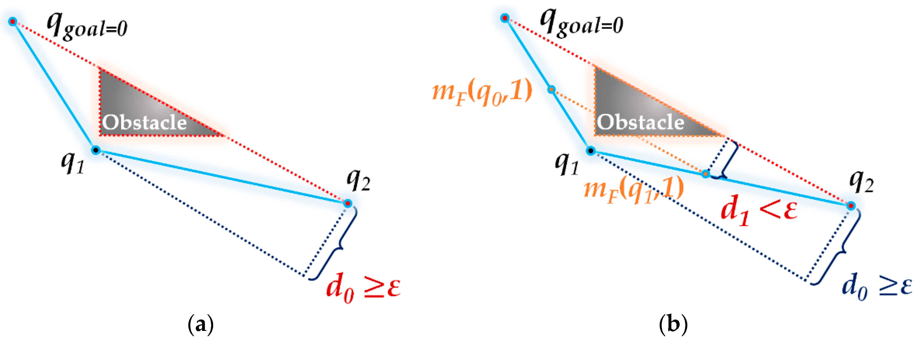
This post triangular processing of the midpoint interpolation method was designed based on the polygon approximation algorithm [18,19], so, as shown in Figure 4, the path is calculated through a constant value called ε (the threshold of minimum clearance) (ε > 0). It determines how closely the obstacle is approximated or, in other words, how close to the optimal path it is. Here, in Figure 4, d follows Equation (1):

$$d_n\left(q_i\right)=\{\begin{array}{cc}\hfill \left(d_{n-1}\left(q_i\right)\right)/2,& n>0\\ \hfill \left(2\sqrt{s\left(s-\alpha \right)\left(s-\beta \right)\left(s-\gamma \right)}\right)/\gamma ,& n=0\end{array}\left(s=\left(\alpha +\beta +\gamma \right)/2\right)$$

(1)

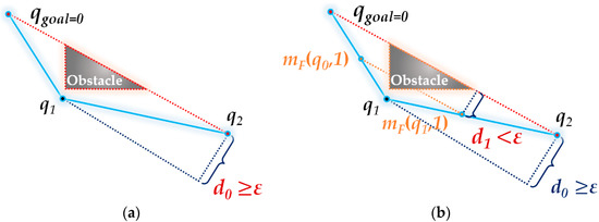
Figure 4. Interpolation function of post triangular processing of the midpoint interpolation method: (a) height d₀ of the triangle formed by waypoints q₀, q₁, and q₂ of the path is greater than ε (interpolation continuation); (b) height d₁ of the triangle formed by midpoints m_F(q₀,1) and q₁ of q₀ and q₁ and midpoint m_F(q₀,1) is the midpoint of q₀ and q₁, also m_F(q₁,1) is the midpoint of q₁ and q_2.

Here, ξ() is a function that receives the node as a variable and returns the parent node of that node. The n-squared (n ≥ 0) of the ξ() function can be expressed as ${\xi }^n\left(q_i\right):=\stackrel{n}{\overbrace{(\xi \circ \xi \circ \dots \circ \xi )}}(q_i)$, and if n is 0,${\xi }^0\left(q_i\right):=q_i$ holds.

For the waypoint q_i, the value of d decreases by 1/2 as interpolation proceeds (n). The initial value d₀ is the height of the triangle formed by the three line segments α, β, and γ (γ < α + β), and the value of d_n becomes (d_n−1)/2. Based on q_i, let α be the line segment from itself to the parent node, β be the line segment from the parent node to the grandparent node, and γ be the line segment from itself to the grandparent node. This d value serves as a measure to confirm the clearance of the obstacle compared to ε. This is because the smaller the d, the closer the path is to the obstacle.

Equation (1) converges to 0 when n becomes infinitely large in d_n, so epsilon receives only a value greater than 0 (positive number) from the user. ε is always greater than d_n when n is infinitely large. i.e., d is always smaller than epsilon at some point when n becomes infinitely large. This can be expressed as Equations (2) and (3) as follows:

$$\underset{n\to \infty }{\lim }{d}_n\left(q_i\right)=\underset{n\to \infty }{\lim }\frac{d_{n-1}\left(q_i\right)}{2}=\underset{n\to \infty }{\lim }\frac{d_0\left(q_i\right)}{2^n}=\underset{n\to \infty }{\lim }\frac{ℂ}{2^n}=0,$$

(2)

$$\therefore \underset{n\to \infty }{\lim }{d}_n\left(q_i\right)=0,\epsilon >0\to \epsilon >\underset{n\to \infty }{\lim }{d}_n\left(q_i\right).$$

(3)

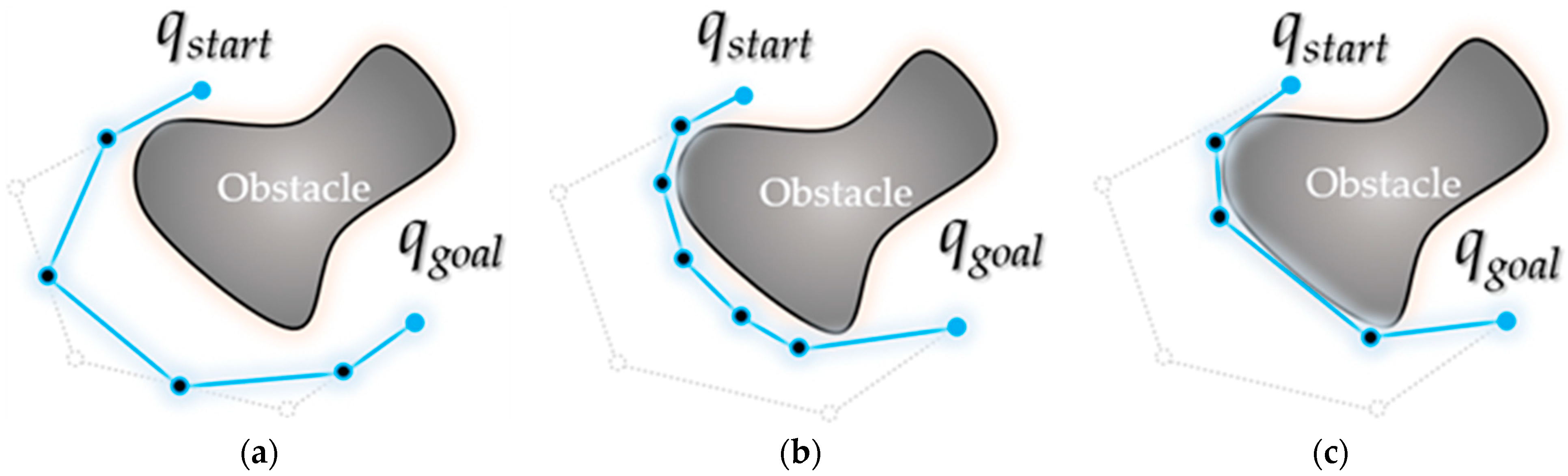
However, since optimality and clearance are opposite attributes, the closer ε is to 0 as shown in Figure 5, the more similar the path or path length is to the visibility graph, but it is not a smooth path [20]. The farther away it is from 0 (within a significant value where the path is modified), the farther it is from the optimum, but a smooth (kinetic) path is made, so ε should be set to a suitable value according to the environment.

Figure 5. Variations according to ε values in post triangular processing of midpoint interpolation method (ε value of (a) > ε value of (b) > ε value of (c)): (a) When ε value is set relatively large; (b) When ε value is set relatively medium (smooth path); (c) When ε value is set relatively small (closer to the optimal path).

The following Algorithm 3 shows the pseudocode of the proposed post triangular processing of the midpoint interpolation method. It is mainly composed of the post triangular function (Algorithm 4) and interpolation function (Algorithm 5).

Algorithm 3 Pseudocode of Proposed Post Triangular Processing of Midpoint Interpolation Method
Input:
R ← path from {RRT/ …}
C ← position set of all (measured) boundary points in all (known) obstacles
ε ← threshold value of minimum clearance
Output:
R ← modified path R
Initialize:
fmodify ← true
ProcedurepostTriProcOfMidInterpolation
Begin
1	WhilefmodifyDo
2	fmodify ← false   // is the path modified
3	t ← 0   // index of the currently focused point
4	qchild ← first point in R
5	qparent ← next point of qchild in R
6	While not [qparent is the last point in R] Do
7	qancestor ← next point of qparent in R
8	If not isTrapped(qchild, qancestor, C) Then
10	R ← postTriangular(R, ε, t, fmodify)
11	Else
12	R ← interpolation(R, C, ε, t, fmodify)
13	qchild ← t-th point in R
14	qparent ← next point of qchild in R
End

The input values of the post triangular processing of the midpoint interpolation method consist of the path R planned through a path planning algorithm, such as the RRT algorithm, the obstacle area information C, and the threshold value ε of the minimum clearance.

The f_modify is a variable that determines whether the input path R has been modified by this method, and if the path is modified even once, the entire process is repeated. If the path modification does not occur in the process of repeating, the algorithm is terminated. t refers to the index of the currently focused waypoint of R. That is, if t is 0, it is the starting point, which is the first point of R.

In R, when the first focusing point is q_child, the next point of that point q_child is q_parent, and the next point of that point q_parent is q_ancestor. It is determined whether the distance between q_child and q_ancestor is free from obstacle collision (isTrapped() function). If it is free from collision, it is called postTriangular(); otherwise, it is called interpolation(). postTriangular() connects q_child and q_ancestor as in the triangular rewiring method [8], and the q_parent between them is deleted from the path. interpolation() finds (interpolates) the points between q_child and q_parent and between q_parent and q_ancestor that are free from obstacle collision when connected and rewires q_child, q_ancestor, and those two points are found. If R and t are updated due to postTriangular() or interpolation(), q_child (the t-th waypoint of R), q_parent, and q_ancestor are updated accordingly. If q_parent is the last point in R, f_modify is checked. Otherwise, the above process is repeated for the updated q_child and q_ancestor.

Here, path modification by postTriangular() deletes the waypoints and makes a more optimal path but has the effect of sharpening the path shape, and path modification by interpolation() creates a new waypoint between the waypoints. Adding/inserting has the effect of making a more optimal path while also smoothing the path shape. Of course, due to the effect of making a more optimal path, path modification by postTriangular() is more efficient than that by interpolation().

Algorithm 4 Pseudocode of Proposed Post Triangular Function
Input:
R ← path R from postTriProcOfMidInterpolation
t ← point index t from postTriProcOfMidInterpolation
fmodify ← boolean fmodify from postTriProcOfMidInterpolation
Output:
R ← modified path R
fmodify ← result of boolean fmodify  //return by reference
Procedure postTriangular From postTriProcOfMidInterpolation
Begin
1	qchild ← t-th point in R
2	qparent ← next point of qchild in R
3	qancestor ← next point of qparent in R
4	R ← Delete path<qchild, qparent> and path<qparent, qancestor> from R
5	R ← Insert path<qchild, qancestor> to R
6	fmodify ← true
End

The input values of postTriangular() of the post triangular processing of the midpoint interpolation method consist of the path R, the focusing point index t, and the path modification f_modify from the post triangular processing of midpoint interpolation method.

Rewiring is performed on the t-th waypoint q_child of R, the next point q_parent, and the next point q_ancestor of that point again. First, the path between q_child and q_parent and the path between q_parent and q_ancestor are deleted. Then the path is inserted between q_child and q_ancestor. Finally, f_modify returns “true” because the path has been modified. Here, Path <A, B> means a partial path from Waypoint A to Waypoint B in the complete path.

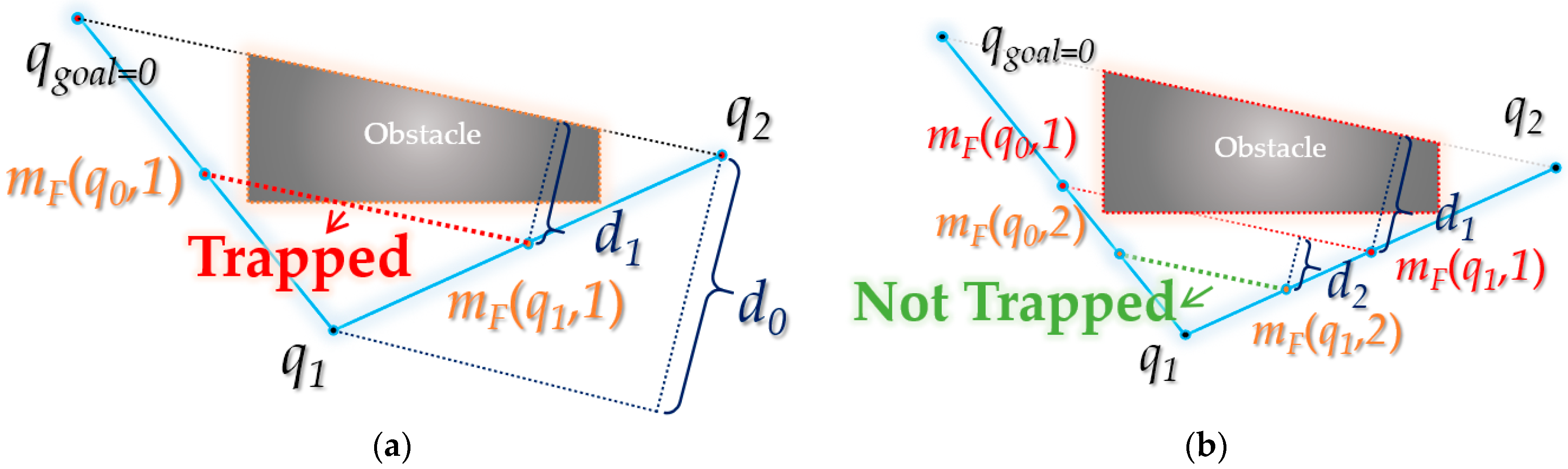
The goal of the proposed post triangular processing of midpoint interpolation method is to find an interpolation point (m_F(q₀), m_F(q₁)) free from obstacle collisions between waypoints (q₀~q₁, q₁~q₂) while descending in the direction of the midpoint (q₁), as shown in Figure 6 in the interpolation process.

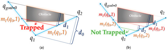
Figure 6. Details of post triangular processing of the midpoint interpolation method: (a) midpoint m_F(q₀,1) of waypoint q₀, q₁ of path and midpoint m_F(q₁,1) of q₁, q₂ are not free from obstacle collision; (b) midpoint m_F(q₀,2) of interpolation point m_F(q₀,1), q₁ and midpoint m_F(q₁,2) between q₁, interpolation point m_F(q₁,1) is free from obstacle collision.

However, the interpolation point m_F follows Equation (4):

$$m_F\left(q_i,k\right)=\{\begin{array}{cc}(\frac{m_F\left(q_i,k-1\right).x+\zeta \left(q_i\right).x}{2},\frac{m_F\left(q_i,k-1\right).y+\zeta \left(q_i\right).y}{2}),\hfill & k>0\hfill \\ \hfill q_i,& k=0\hfill \end{array}$$

(4)

When the k-th interpolation point of the interpolation point q_i is m_F(q_i,k), the 0-th interpolation point becomes itself q_i, and the first interpolation point is the midpoint of q_i and the point ξ(q_i) next to q_i, and the second interpolation point becomes the midpoint of m_F (q_i,1) and ξ(q_i). That is, m_F(q_i,k) (k > 0) becomes the midpoint between m_F(q_i,k − 1) and ξ(q_i). The following Algorithm 5 shows the pseudocode of interpolation() of the proposed post triangular processing of the midpoint interpolation method.

Algorithm 5 Pseudocode of Proposed Interpolation Function
Input:
R ← path R from postTriProcOfMidInterpolation
C ← position set C from postTriProcOfMidInterpolation
ε ← threshold value ε from postTriProcOfMidInterpolation
t ← point index t from postTriProcOfMidInterpolation
fmodify ← boolean fmodify from postTriProcOfMidInterpolation
Output:
R ← modified path R
t ← updated point index t   // return by reference
fmodify ← result of boolean fmodify   // return by reference
Initialize:
qchild ← t-th point in R
qparent ← next point of qchild in R
qancestor ← next point of qparent in R
ProcedureinterpolationFrompostTriProcOfMidInterpolation
Begin
1	d ← altitude of the triangle consisting of qchild, qparent, and qancestor with base <qchild, qancestor>
2	ma ← midpoint between qchild and qparent
3	mb ← midpoint between qparent and qancestor
4	While true Do
5	If d >= ε Then
6	If not isTrapped(ma, mb, C) Then
7	R ← Delete path<qchild, qparent> and path<qparent, qancestor> from R
8	R ← Insert path<qchild, ma>, path<ma, mb>, and path<mb, qancestor> to R
9	fmodify ← true
10	Break
11	Else
12	d ← d / 2
13	ma ← midpoint between ma and qparent
14	mb ← midpoint between mb and qparent
15	Else
16	t ← t + 1
17	Break
End

The input values of interpolation() of the post triangular processing of midpoint interpolation method consist of the path R, the obstacle area information C, the focusing point index t, and the path modification f_modify from the post triangular processing of the midpoint interpolation method.

From the t-th waypoint q_child of R, the next point q_parent, and the next point q_ancestor of that point, the height d of the triangle is obtained, m_a is the midpoint of q_child and q_parent, and m_b is the midpoint of q_parent and q_ancestor. If the path between m_a and m_b is free from obstacle collision (isTrapped()), the path between q_child and q_parent is deleted, and the path between q_child and m_a, the path between m_a and m_b, and the path between m_b and q_ancestor are inserted. Moreover, since the path is modified, f_modify returns “true,” and the method terminates. If the line segment between m_a and m_b is not free from obstacles, the value of d decreases by 1/2, m_a is updated to the midpoint of m_a and q_parent, and m_b is updated to the midpoint of m_b and q_parent. It is then determined whether m_a and m_b are free from obstacles again. This repeated process proceeds until a case is found in which m_a and m_b are free from obstacles or d becomes smaller than ε. If d becomes smaller than ε, the value of t is increased by 1 and the method is terminated.

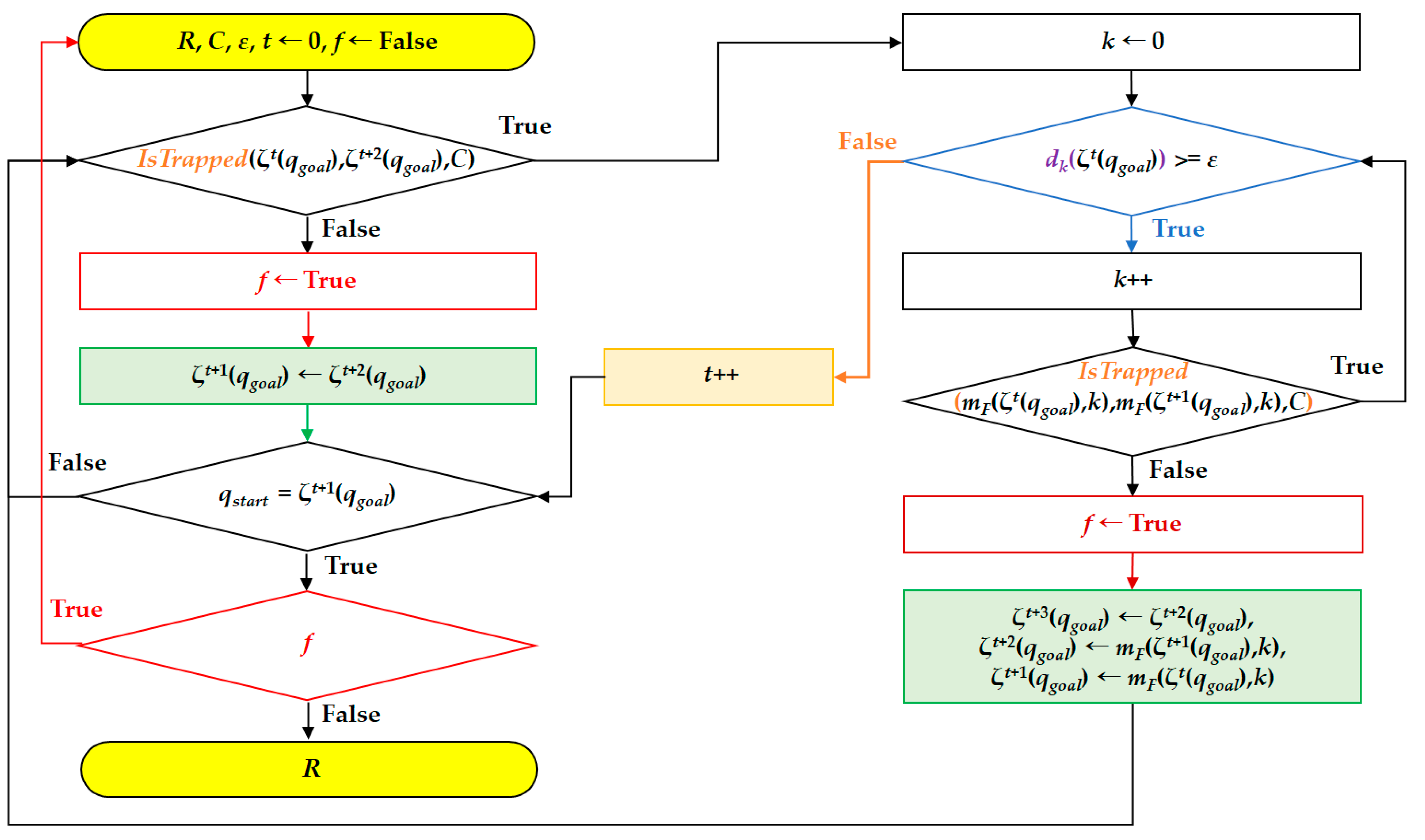
Figure 7 shows the overall flowchart of the proposed post triangular processing of the midpoint interpolation method. Here, ξ^t(q_goal) denotes the t-th next waypoint from the starting point q_goal of the path R, and ξ^t+n(q_goal) is the n-th next waypoint in the ξ^t(q_goal). That is, there are n waypoints between ξ^t(q_goal) and ξ^t+n(q_goal). In the flowchart shown in Figure 7, the stop condition follows the sequence:

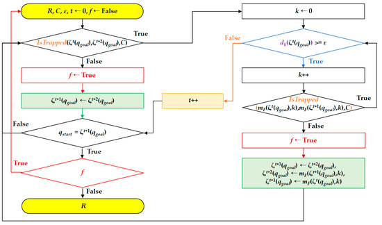
Figure 7. Flowchart of post triangular processing of midpoint interpolation method.

• Check whether the t-th ancestor node and the (t + 2)-th ancestor node of q_goal are collision-free (Here, when t is 0, the 0-th ancestor means itself(q_goal)).
• If the result of Step 1 is not collision-free, compare the d_k(ξ^t(q_goal)) value of the t-th ancestor node of q_goal with ε.
• If d_k(ξ^t(q_goal)) is less than ε, the value of t is incremented by 1, and if the parent node (t + 1) of the t-th ancestor node of q_goal after t is incremented is q_start, the algorithm is stopped (if f is False).

The stopping criterion of the proposed algorithm is based on ε. As shown in Figure 4 and Figure 7, when the value of d_k(ξ^t(q_goal)) becomes smaller than the ε, the algorithm stops the loop. As Equations (1) and (2) and Figure 6 show, the value d_k(ξ^t(q_goal)) decreases deterministically.

4. Experimental Results

The path between the RRT in various environment maps through simulation and the RRT algorithm to which the proposed post triangular processing of the midpoint interpolation method is applied were used to validate the performance of the method proposed in this paper, and the path planning results were compared.

The performance measures compared were the average values after repeating the trial 100 times (sampling position was changed for each trial) of the path length (px) and the planning time (ms) of the first complete path (the first complete path to reach a destination point from a starting point).

Various environment maps have been examined and used to validate the performance of the proposed path planning algorithms in related works. Since the efficiency of the performance measures expected during the experiment varies somewhat based on the composition of obstacles (e.g., number, location, shape), it is important to choose which environment map to utilize carefully.

The four environment maps used in the experiment are shown in Figure 8. The four environment maps were created by partially referring to the experimental environment proposed by Han in 2017 [21]. All environment maps were 600 × 600 px in size, with a 30 px step length. The start points (S) are represented by green circles, while the destination points (G) are represented by purple circles. Obstacles are black polygons with yellow contours (blue in the experimental results).

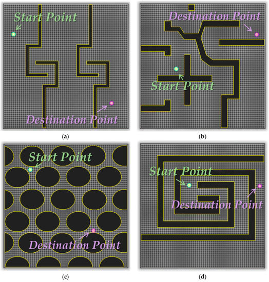
Figure 8. Environment maps for experiments: (a) Map 1; (b) Map 2; (c) Map 3; (d) Map 4.

Map 1 of Figure 8a appears to be an efficient environment for validating optimality and completeness but a weak environment for sampling-based path planning algorithms like the RRT algorithm. Many samplings are required since the probability of finding a solution is low. Map 2 of Figure 8b appears to be an efficient environment for validating the optimality and completeness of the path planning algorithm. Map 3 of Figure 8c is an environment that is efficient for validating the optimality and the planning time of the path planning algorithm, as it consists of obstacles (50 vertices) that approximate circles. Map 4 of Figure 8d is an environment that is efficient for validating the optimality and the planning time of the path planning algorithm but a weak environment for sampling-based path planning algorithms such as the RRT algorithm.

The number of samples and planning time required increase drastically when the path to the destination point is narrow or there are few entrances since the sampling-based path planning algorithm depends on probabilistic completeness.

The specification of the computer used in the simulation is shown in Table 1. The simulator used for the simulation [8] was developed based on C# WPF (Microsoft Visual Studio Community 2019 Version 16.1.6 Microsoft .NET Framework Version 4.8.03752), and only a single thread was used for calculations except for the visual part. Generally, depending on the specification of the computer, the result of performance measurements, such as planning time, may vary during the simulation.

Table 1. Computer performance for simulation.

H/W	Specification
CPU	Intel Core i7-6700k 4.00 GHz (8 CPUs)
RAM	32,768 MB (32 GB DDR4)

We validate the experimental results (path length, planning time) in the four environment maps in which the post triangular processing of the midpoint interpolation method (ε: 50, 30, 10 px) is applied to the RRT algorithm and its path planning results. Since ε requires a higher amount of computation as it gets smaller, it was set to a value close to the 30 px step length of the experimental environment.

The experimental results for each map consist of a figure and table. The figure is a path planning result for each algorithm shown in the case of a single trial (the figure for each algorithm is not the result of repeated trials). The table shows an average value of the results of planning time and path length from the path planning repeated trials. There may be a significant difference between the performance observed visually and the numerical results in the table for one of the repeated trials. The form of the planned path for each algorithm is shown in the figure for visual reference. Furthermore, the proposed post triangular processing of the midpoint interpolation method is used to see whether there is a region where the piecewise linear path is smoothed.

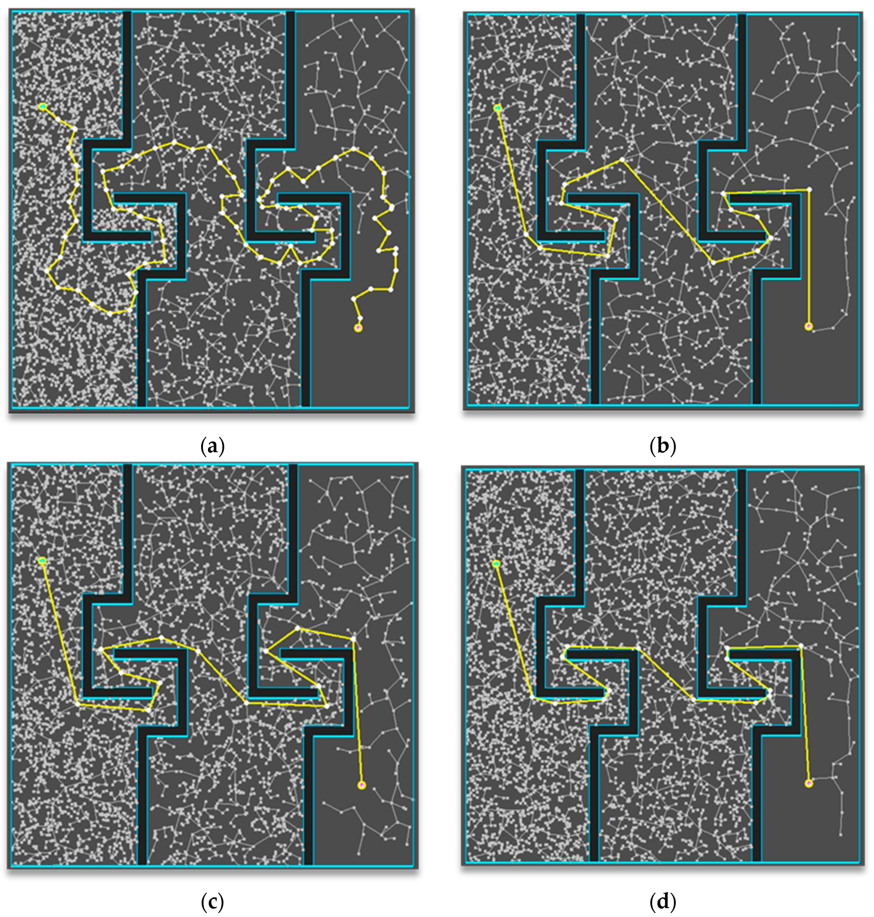
The path planning results are shown in Figure 9 for Map 1 among the specified environment maps for each algorithm. In terms of appearance, the one to which the post triangular processing of the midpoint interpolation method (ε: 10 px) was applied seems to have a smoother slope compared to those of the other algorithms, and the path length with the method (ε: 10 px) seems to be the shortest.

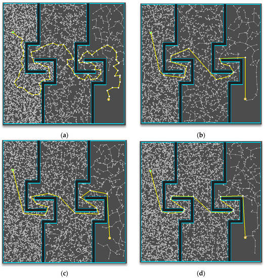
Figure 9. Experimental results of Map 1: (a) RRT; (b) proposed method (ε: 50 px) applied; (c) proposed method (ε: 30 px) applied; (d) proposed method (ε: 10 px) applied.

The path planning results (average values after repeating the trial 100 times) are shown in Table 2 for Map 1 among the specified environment maps for each algorithm. When applying the post triangular processing of the midpoint interpolation method (ε: 10 px), the path length becomes 62% (1224/1994(%)) compared to the RRT, which is the shortest of all the algorithms, and the planning times are all similar.

Table 2. Experimental results of Map 1 (numbers in parentheses (averages of repeating trial 100 times) are relative ratios to RRT results (values less than 1 are counted as 1)).

Performance	RRT	Proposed Method (ε: 50 px)	Proposed Method (ε: 30 px)	Proposed Method (ε: 10 px)
Path length (px)	1944 (100%)	1403 (72%)	1325 (68%)	1224 (62%)
Planning time (ms)	697 (100%)	698 (100%)	698 (100%)	698 (100%)

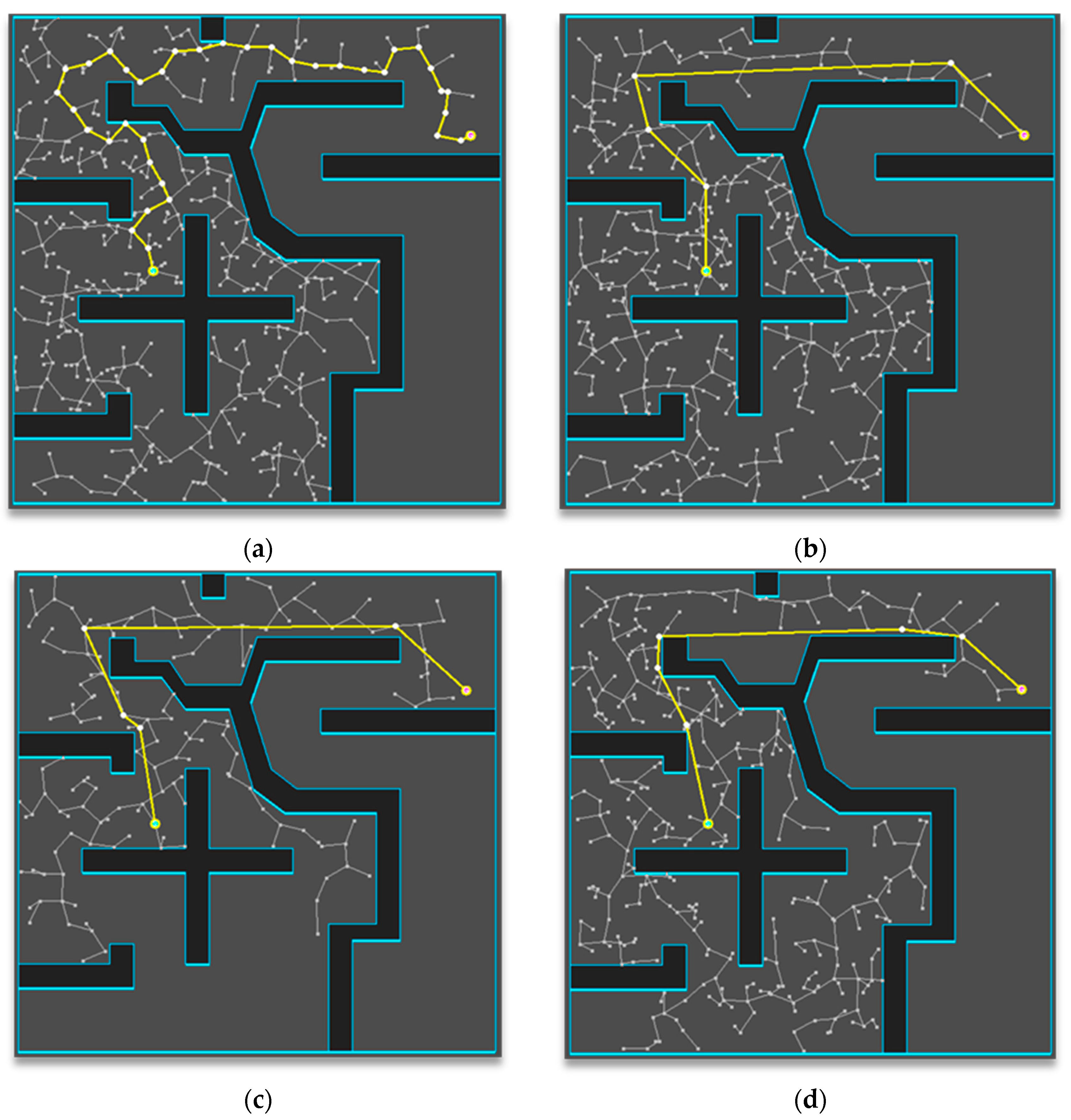
The path planning results are shown in Figure 10 for Map 2 among the specified environment maps for each algorithm. In terms of appearance, the one to which the post triangular processing of midpoint interpolation method (ε: 10 px) was applied seems to have a smoother slope compared to those of the other algorithms, and the path length with the method (ε: 10 px) seems to be the shortest.

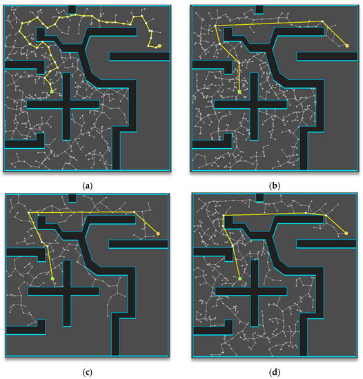
Figure 10. Experimental results of Map 2: (a) RRT; (b) Proposed method (ε: 50 px) applied; (c) Proposed method (ε: 30 px) applied; (d) Proposed method (ε: 10 px) applied.

The path planning results (average values after repeating the trial 100 times) are shown in Table 3 for Map 2 among the specified environment maps for each algorithm. By applying the post triangular processing of midpoint interpolation method (ε: 10 px), the path length becomes 74% (730/986(%)) compared to the RRT, which is the shortest of all the algorithms, and the planning time is similar to that of the RRT algorithm when the method (ε: 50 px) is applied. However, the absolute time difference is 1 ms, which seems to be large when the method is applied because it is an environment that requires less planning time.

Table 3. Experimental results of Map 2 (numbers in parentheses (averages of repeating trial 100 times) are relative ratios to RRT results (values less than 1 are counted as 1)).

Performance	RRT	Proposed Method (ε: 50 px)	Proposed Method (ε: 30 px)	Proposed Method (ε: 10 px)
Path length (px)	986 (100%)	780 (79%)	752 (76%)	730 (74%)
Planning time (ms)	10 (100%)	10 (100%)	11 (110%)	11 (110%)

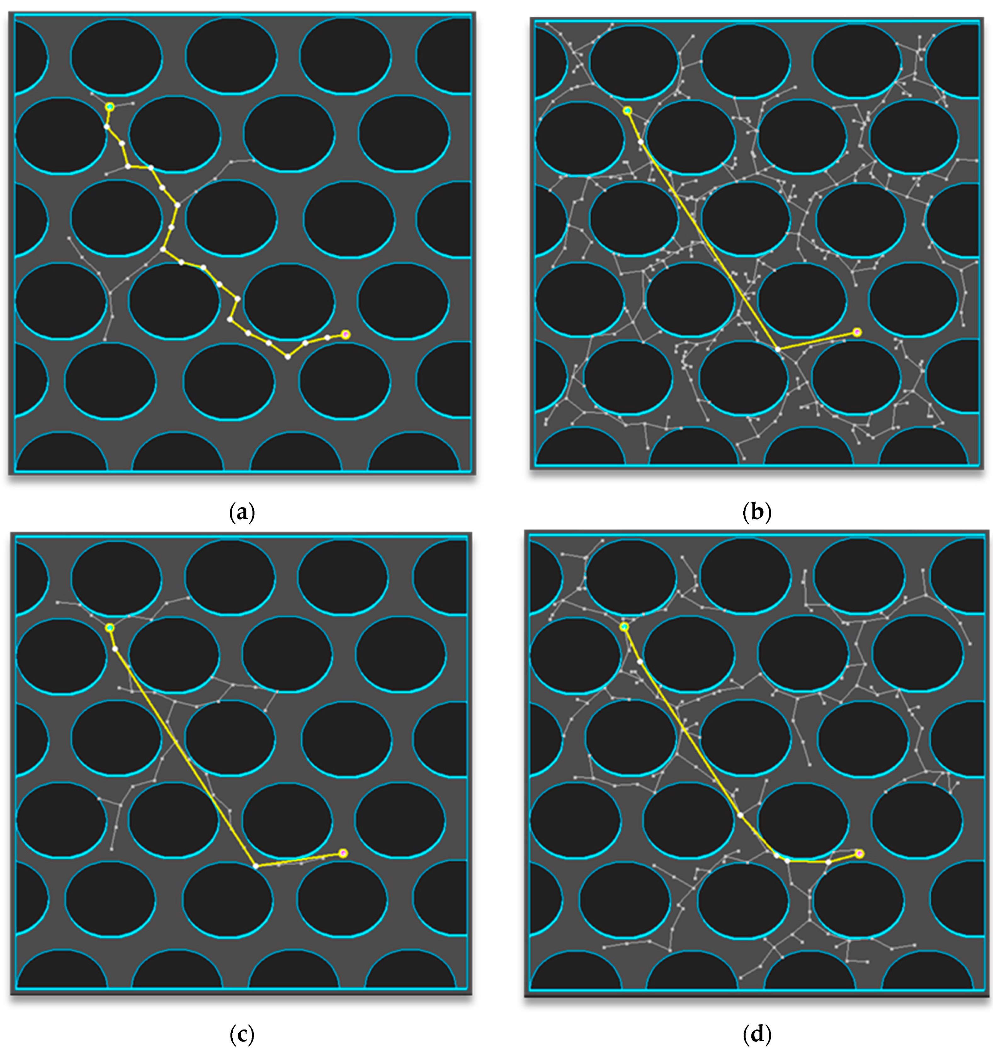
The path planning results are shown in Figure 11 for Map 3 among the specified environment maps for each algorithm. In terms of appearance, the one to which the post triangular processing of midpoint interpolation method (ε: 10 px) was applied seems to have a smoother slope compared to those of the other algorithms, and the path length with the method (ε: 10 px) seems to be the shortest.

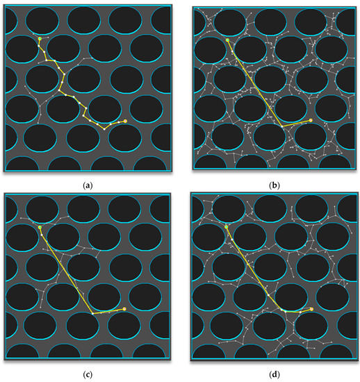
Figure 11. Experimental results of Map 3: (a) RRT; (b) Proposed method (ε: 50 px) applied; (c) Proposed method (ε: 30 px) applied; (d) Proposed method (ε: 10 px) applied.

The path planning results (average values after repeating the trial 100 times) are shown in Table 4 for Map 3 among the specified environment maps for each algorithm. By applying the post triangular processing of midpoint interpolation method (ε: 10 px), the path length becomes 82% (505/613(%)) compared to the RRT, which is the shortest of all the algorithms, and the planning time is the most similar to that of the method (ε: 10 px), as it takes 16% more time than the RRT algorithm. However, the absolute time difference is 2 ms, and since it is an environment that requires less planning time, the difference appears to be large when the method is applied.

Table 4. Experimental results of Map 3 (numbers in parentheses (averages of repeating 100 times) are relative ratios to the RRT results (values less than 1 are counted as 1)).

Performance	RRT	Proposed Method (ε: 50 px)	Proposed Method (ε: 30 px)	Proposed Method (ε: 10 px)
Path length (px)	613 (100%)	535 (87%)	512 (83%)	505 (82%)
Planning time (ms)	6 (100%)	7 (116%)	8 (133%)	8 (133%)

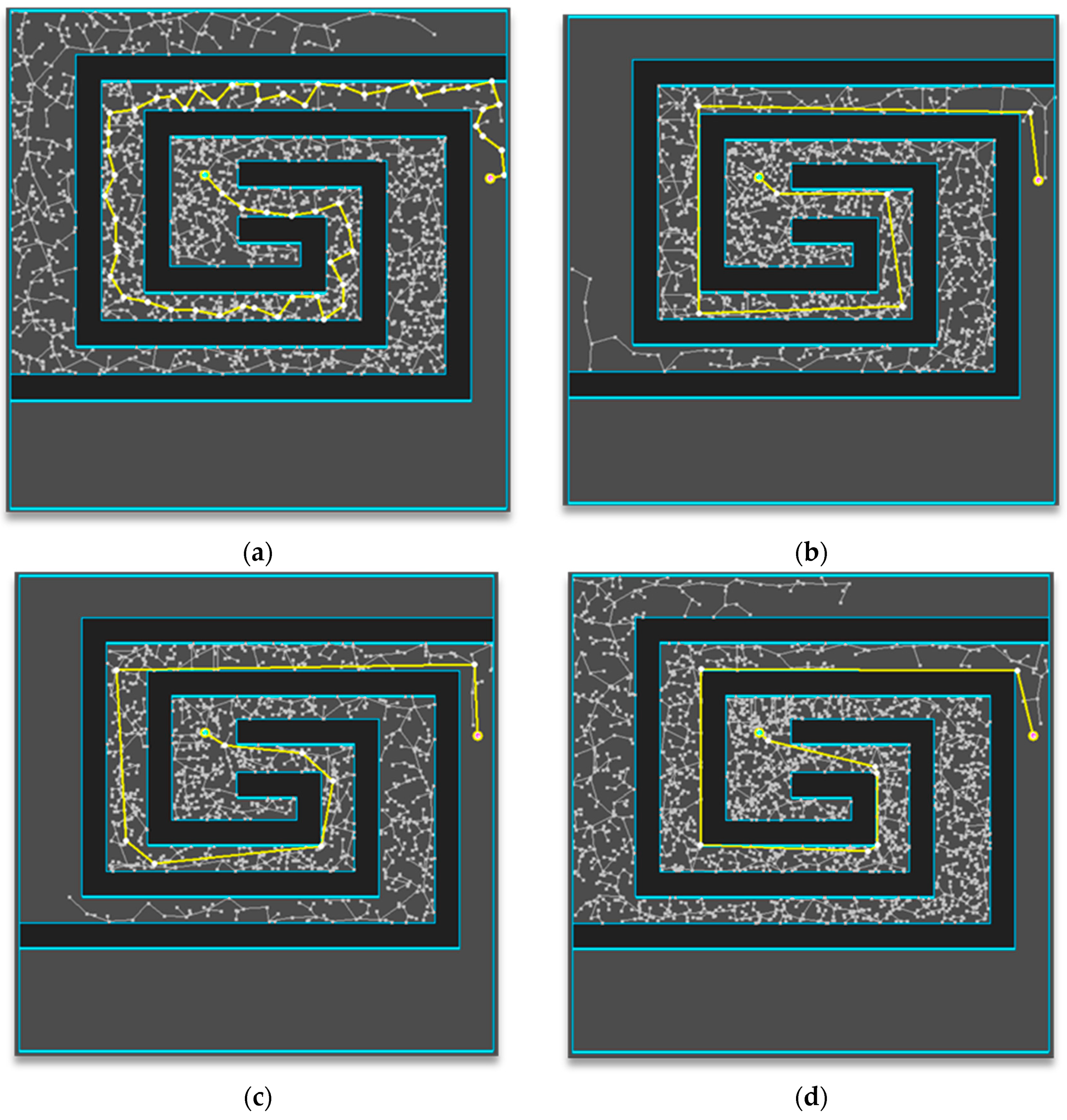
The path planning results are shown in Figure 12 for Map 4 among the specified environment maps for each algorithm. In terms of appearance, the one to which the post triangular processing of the midpoint interpolation method (ε: 30 px) was applied seems to have a smoother slope compared to those of the other algorithms, and the path length with the method (ε: 10 px) seems to be the shortest.

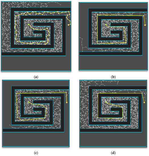
Figure 12. Experimental results of Map 4: (a) RRT; (b) Proposed method (ε: 50 px) applied; (c) Proposed method (ε: 30 px) applied; (d) Proposed method (ε: 10 px) applied.

The path planning results (average values after repeating the trial 100 times) are shown in Table 5 for Map 4 among the specified environment maps for each algorithm. By applying the post triangular processing of the midpoint interpolation method (ε: 10 px), the path length becomes 77% (1190/1536(%)) compared to the RRT, which is the shortest of all the algorithms, and all the planning times are similar.

Table 5. Experimental results of Map 4 (numbers in parentheses to (averages of repeating 100 times) are relative ratios to RRT results (values less than 1 are counted as 1)).

Performance	RRT	Proposed Method (ε: 50 px)	Proposed Method (ε: 30 px)	Proposed Method (ε: 10 px)
Path length (px)	1536 (100%)	1284 (83%)	1261 (82%)	1190 (77%)
Planning time (ms)	1752 (100%)	1753 (100%)	1753 (100%)	1753 (100%)

Consequently, the post triangular processing of the midpoint interpolation method (ε: 10 px) performed well in the path length aspect for all maps, demonstrating that the proposed method is efficient in terms of optimality.

5. Conclusions

In this research, the post triangular processing of the midpoint interpolation method minimized the planning time and shortened the path length of the sampling-based algorithm.

The proposed post triangular processing of the midpoint interpolation method was closer to the optimal path and somewhat solved the sharp path problem through the interpolation process. Furthermore, all path planning algorithms that plan a locally piecewise linear path could apply the proposed algorithm. This strength has significance in that it can be applied not only to the algorithm presented in this paper but also to various path planning algorithms. We validated the performance of the proposed method after it was applied to the RRT algorithm and its path planning results through simulation. It was verified that the path length was shortened by 18–38% (average 26%) depending on the threshold ε when applied to the RRT algorithm in the four different environment maps. As a result, the RRT algorithm applying the proposed post triangular processing of the midpoint interpolation method showed a more optimal path.

The proposed post triangular processing of the midpoint interpolation method is based on a general global planning case in which a robot first discovers a global path from its start point to its destination point before beginning to navigate. In dynamic environments, not only local planners but also global planners must deal with kinodynamic problems in real-time. Furthermore, the method proposed in this paper is more efficient in terms of the optimality of robot path planning, but optimality is not guaranteed. Future work should determine how to make a path that is closer to the optimal path.

References

- Lindner, L.; Sergiyenko, O.; Moises, R.L.; Ivanov, M.; Julio, C.R.Q.; Daniel, H.B.; Wendy, F.F.; Vera, T.; Fabian, N.M.R.; Mercorelli, P. Machine Vision System Errors for Unmanned Aerial Vehicle Navigation. In Proceedings of the IEEE International Symposium on Industrial Electronics, Edinburgh, UK, 19–21 June 2017; pp. 1615–1620. [Google Scholar]
- Sergiyenko, O.; Wendy, F.F.; Mercorelli, P. Machine Vision and Navigation, 1st ed.; Springer: Cham, Switzerland, 2020. [Google Scholar]
- Abdi, A.; Adhikari, D.; Park, J.H. A novel hybrid path planning method based on q-learning and neural network for robot arm. Appl. Sci. 2021, 11, 6770. [Google Scholar] [CrossRef]
- Schwab, K. The Fourth Industrial Revolution, 1st ed.; Crown Business: New York, NY, USA, 2017. [Google Scholar]
- Wang, X.; Luo, X.; Han, B.; Chen, Y.; Liang, G.; Zheng, K. Collision-free path planning method for robots based on an improved rapidly-exploring random tree algorithm. Appl. Sci. 2020, 10, 1381. [Google Scholar] [CrossRef] [Green Version]
- LaValle, S.M.; Kuffner, J.J., Jr. Randomized kinodynamic planning. Int. J. Robot. Res. 2001, 20, 378–400. [Google Scholar] [CrossRef]
- Kuffner, J.J., Jr.; LaValle, S.M. RRT-Connect: An Efficient Approach to Single-Query Path Planning. In Proceedings of the IEEE International Conference on Robotics and Automation, San Francisco, CA, USA, 24–28 April 2000; Volume 2, pp. 995–1001. [Google Scholar]
- Kang, J.-G.; Lim, D.-W.; Choi, Y.-S.; Jang, W.-J.; Jung, J.-W. Improved RRT-connect algorithm based on triangular inequality for robot path planning. Sensors 2021, 21, 333–364. [Google Scholar] [CrossRef] [PubMed]
- Roy, D. Visibility graph based spatial path planning of robots using configuration space algorithms. Robot. Auton. Syst. 2009, 24, 1–9. [Google Scholar] [CrossRef]
- Katevas, N.I.; Tzafestas, S.G.; Pnevmatikatos, C.G. The approximate cell decomposition with local node refinement global path planning algorithm: Path nodes refinement and curve parametric interpolation. J. Intell. Robot. Syst. 1998, 22, 289–314. [Google Scholar] [CrossRef]
- Warren, C.W. Global Path Planning using Artificial Potential Fields. In Proceedings of the International Conference on Robotics and Automation, Scottsdale, AZ, USA, 14–19 May 1989; Volume 1, pp. 316–321. [Google Scholar]
- LaValle, S.M. Rapidly-Exploring Random Trees: A New Tool for Path Planning; Springer: London, UK, 1998. [Google Scholar]
- Karaman, S.; Frazzoli, E. Sampling based algorithms for optimal motion planning. Int. J. Robot. Res. 2011, 30, 846–894. [Google Scholar] [CrossRef]
- Gammell, J.D.; Srinivasa, S.S.; Barfoot, T.D. Informed RRT*: Optimal Sampling based Path Planning Focused via Direct Sampling of an Admissible Ellipsoidal Heuristic. In Proceedings of the IEEE/RSJ International Conference on Intelligent Robots and Systems, Chicago, IL, USA, 14–18 September 2014; pp. 2997–3004. [Google Scholar]
- Klemm, S.; Oberländer, J.; Hermann, A.; Roennau, A.; Schamm, T.; Zollner, J.M.; Dillmann, R. RRT*-Connect: Faster, Asymptotically Optimal Motion Planning. In Proceedings of the IEEE International Conference on Robotics and Biomimetics, Zhuhai, China, 6–9 December 2015; pp. 1670–1677. [Google Scholar]
- Islam, F.; Nasir, J.; Malik, U.; Ayaz, Y.; Hasan, O. Rrt*-smart: Rapid Convergence Implementation of rrt* towards Optimal Solution. In Proceedings of the IEEE International Conference on Mechatronics and Automation, Chengdu, China, 5–8 August 2012; pp. 1651–1656. [Google Scholar]
- Jeong, I.-B.; Lee, S.-J.; Kim, J.-H. Quick-RRT*: Triangular inequality based implementation of RRT* with improved initial solution and convergence rate. Expert Syst. Appl. 2019, 123, 82–90. [Google Scholar] [CrossRef]
- Jung, J.-W.; So, B.-C.; Kang, J.-G.; Lim, D.-W.; Son, Y. Expanded Douglas–Peucker polygonal approximation and opposite angle based exact cell decomposition for path planning with curvilinear obstacles. Appl. Sci. 2019, 9, 638. [Google Scholar] [CrossRef] [Green Version]
- Jung, J.-W.; So, B.-C.; Kang, J.-G.; Jang, W.-J. Circumscribed Douglas-Peucker Polygonal Approximation for Curvilinear Obstacle Representation. In Proceedings of the IEEE 2019 7th International Conference on Robot Intelligence Technology and Applications (RiTA), Daejeon, Korea, 1–3 November 2019; pp. 237–241. [Google Scholar]
- Kwon, J.; Choi, K. Kinodynamic model identification: A unified geometric approach. IEEE Trans. Robot. 2021, 37, 1100–1114. [Google Scholar] [CrossRef]
- Han, J. Mobile robot path planning with surrounding point set and path improvement. Appl. Soft Comput. 2017, 57, 35–47. [Google Scholar] [CrossRef]
Publisher’s Note: MDPI stays neutral with regard to jurisdictional claims in published maps and institutional affiliations. |
© 2021 by the authors. Licensee MDPI, Basel, Switzerland. This article is an open access article distributed under the terms and conditions of the Creative Commons Attribution (CC BY) license (https://creativecommons.org/licenses/by/4.0/).