
Non-Classic Atmospheric Optical Turbulence: Review

1
Department of Physics, University of Miami, Coral Gables, FL 33146, USA
2
Fraunhofer IOSB, Fraunhofer Institute of Optronics, System Technologies and Image Exploitation, Gutleuthausstr. 1, 76275 Ettlingen, Germany
*
Author to whom correspondence should be addressed.
Appl. Sci. 2021, 11(18), 8487; https://doi.org/10.3390/app11188487
Submission received: 19 July 2021
/
Revised: 1 September 2021
/
Accepted: 3 September 2021
/
Published: 13 September 2021
(This article belongs to the Special Issue Atmospheric Optics Sensing, Mitigation and Exploitation)
Abstract
:Theoretical models and results of experimental campaigns relating to non-classic regimes occurring in atmospheric optical turbulence are overviewed. Non-classic turbulence may manifest itself through such phenomena as a varying power law of the refractive-index power spectrum, anisotropy, the presence of constant-temperature gradients and coherent structures. A brief historical introduction to the theories of optical turbulence, both classic and non-classic, is first presented. The effects of non-classic atmospheric turbulence on propagating light beams are then discussed, followed by the summary of results on measuring the non-classic turbulence, on its computer and in-lab simulations and its controlled synthesis. The general theory based on the extended Huygens–Fresnel method, capable of quantifying various effects of non-classic turbulence on propagating optical fields, including the increased light diffraction, beam profile deformations, etc., is then outlined. The review concludes by a summary of optical engineering applications that can be influenced by atmospheric non-classic turbulence, e.g., remote sensing, imaging and wireless optical communication systems. The review makes an accent on the results developed by the authors for the recent AFOSR MURI project on deep turbulence.
1. Introduction
The aim of the introductory section is three-fold: first, outlining the historical development of concepts and parameters characterizing 3D turbulent motion; second, thoroughly familiarizing the reader with the classic theory of turbulence; and third, briefly discussing the 2D turbulence theory being a stand-alone, comprehensive example of non-classic turbulence.
1.1. Early Studies
Leonardo da Vinci was one of the first scholars who attempted to visualize, classify and comprehend the phenomenon of turbulence. Figure 1 shows the drawing that he made in 1509 on recording the experimental observation of water surface turbulence produced by differently shaped objects. The appearance of the turbulent eddies behind the flat obstacle is evident. It is currently argued that Leonardo could have been exposed to ancient books that flooded Italy after the fall of Constantinople earlier in 1453. This suggests that the phenomenon of turbulence could have been appreciated for millennia.
In the middle of the 18th century, Leonard Euler established the broad field of fluid dynamics by introducing a set of partial differential equations governing the motion of incompressible, adiabatic and inviscid flows. The Euler equations are the consequence of the balance between the fluid’s energy and momentum and incorporate the continuity law (conservation of mass) [1]. Almost a century later, Gabriel Stokes derived a set of equations that generalized Euler’s equations to viscous fluids and are now known as the Navier–Stokes equations [2].
By the middle of the 19th century, the interest in turbulence resurfaced. On studying instabilities in the pendulum’s motion, G. Stokes introduced a parameter that characterizes fluid flows by the amount of their mixing [3], currently known as the Reynolds number (after Osborn Reynolds who was the first to make practical use of the concept [4]). The Reynolds number characterizes the ratio of inertial to viscous forces in the fluid:
where u [m/s] is the speed, L [m] is the characteristic linear dimension, and [m/s] is the kinematic viscosity of the fluid. The transition from laminar (mixing-free) to turbulent flows depends on geometry—from to for pipe flow to for boundary layers. In atmospheric cyclones, the number can reach values on the order of .
On developing the tools for weather forecasting, Lewis Fry Richardson came up in the early 1920s with the construction that is now known as the direct energy cascade or Richardson energy cascade [5]. In a classic 3D turbulent flow, the energy is mechanically injected into a volume filled with a fluid by means of a velocity field, such as wind in a gas or a current in a liquid. If the initial distribution of some scalar field (temperature, pressure, concentration of a chemical compound) within the volume is not uniform, the injected energy creates a few sizable eddies, which later break down into a larger number of smaller ones. The process repeats until a sufficiently small scale is reached and the mechanical energy starts dissipating into heat. A turbulent eddy is intuitively understood as a region of space in which the scalar field remains fairly correlated. In 1925, Ludwig Prandtl introduced a parameter, currently known as the Prandtl number, which characterizes the ratio of momentum diffusivity to diffusivity of an advected scalar. It is defined by the following expression: [6]
where [m/s] is the diffusivity relating to the nature of the advected scalar: thermal for temperature advection, mass for molecular advection, etc. This parameter plays a crucial part in characterizing non-classic turbulent regimes. For atmospheric turbulence, the value of Prandtl number is about .
Having been greatly influenced by the work of Richardson, in 1935, Sir Geoffrey Ingram Taylor introduced the concept of locally isotropic 3D turbulence [7], the isotropy (or invariance, in the limit) being understood as the weak dependence of the flow’s characteristics on orientations in space. Taylor is also known for his frozen turbulence hypothesis, suggesting that all the eddies are advected by the mean streamwise velocity without changes in their properties. Using the conception of Taylor, Theodore de Karman and Leslie Howarth introduced the 3D correlation tensor of the turbulent flow and reduced it to a scalar correlation under the isotropy constraint [8].
1.2. Kolmogorov Theory (1941–1942)
After establishing the rigorous, mathematical theory of random functions in 1930s [9,10] Andrey Nikolaevich Kolmogorov and his students attempted its application to isotropic turbulence. Greatly influenced by the results of de Karman and Howarth, Millionshchikov applied the concept of Kolmogorov’s ensemble averages to a homogeneous and isotropic turbulent flow [11]. He also developed the system of equations governing the velocity correlation and implemented quasi-normal approximation to obtain the closed system of the second- and third-order correlations [12].
Between 1941 and 1942, Kolmogorov established the foundations of the classic turbulence theory by formulating three hypotheses regarding the equilibrium regime in a homogeneous turbulent flow at sufficiently high Reynolds numbers and for sufficiently small scales [13,14,15,16,17] (see also important parallel work by Obukhov [18,19,20]). This theory largely elaborated on the Richardson turbulent energy cascade by assigning to a turbulent eddy a scale l, a velocity vector and a time . It was then conjectured that the cascade is formed by the largest eddies, with a scale (integral or outer scale), , L being the scale of entire region of mixing. It can be estimated as follows:
where K is the turbulent kinetic energy (reduced to unit mass) as follows:
and [m s] is the energy dissipation rate. Then, by defining the turbulent Reynolds number as
and applying it to the integral scale, one obtains the following:
attaining very large values.
The first Kolmogorov hypothesis states: (i) the turbulent motion of eddies with scales is statistically isotropic. It appears possible to estimate a threshold scale that separates the regimes with isotropic () and anisotropic () eddy scales, as . The second hypothesis postulates that (ii) the statistics of the small-scale () eddy motion have a universal form that is uniquely determined by ε and ν. This range of scales is also known as the universal equilibrium range. It follows from (ii) that a set of parameters solely depending on and can be introduced:
These are the characteristics of the smallest eddies before dissipation, carrying Kolmogorov’s name. Note that starts at a very large number when energy is injected at scale and decreases to unity at scale . The third hypothesis states that (iii) the statistics of motion of eddies with scales in the range have a universal form that is uniquely determined by ε and are independent of ν.
There is another scale, , that splits the universal dissipation range ) in which motion is the result of viscous forces.
The Kolmogorov theory established the regime of classic turbulence conceptually, and also led to specific mathematical law governing the structure of turbulent velocity correlation function or, equivalently, its energy spectrum. On introducing spatial frequency as (or for dimensionless version) and energy spectrum such that
one finds at once that, in order for to depend on and , i.e., to be in the form
it suffices to perform dimensional analysis. Substituting , , , into the equation above, one finds that and , thereby leading to the famous Kolmogorov law as follows:
where is a data-fitted constant. One may also define the dissipation rate spectrum, [m/s], as follows:
It was estimated that most of the energy (80%) is contained in the energy production range , and most of the dissipation (90%) occurs in the interval . Additionally, in terms of a temporal scale of an eddy, on converting to its lifespan , 90% is spent in the production range and 10% in the inertial range.
1.3. Batchelor-Leigh-Kraichnan Theory
In the late 1960s, Robert Harry Kraichnan [21], Cecil Leith [22] and George Batchelor [23] (see also earlier important work [24]) developed the theory of 2D turbulence. Unlike in the 3D case, in addition to energy K, the turbulent flow must also be characterized by enstrophy (reduced to unit mass):
where is the flow helicity. The power spectra of energy and enstrophy can be shown to be in a simple relation as follows:
Unlike in 3D turbulence, described by the direct turbulent energy cascade, in which the energy is injected at the largest scale and dissipates at the lowest scale, the 2D turbulence is characterized by a dual cascade: the enstrophy undergoes the direct cascade from the intermediate injection scale to the lowest scale, having the power law and the energy exhibits the inverse energy cascade from the intermediate scale to the largest scale, having the same (in form) power law as the classic 3D turbulence.
Even though the 2D turbulence model could not be directly applied to 3D turbulence research and applications, it provided the invaluable insight into both classic and non-classic turbulent regimes and helped in describing various equilibrium and non-equilibrium turbulent regimes, particularly those appearing in rotating and conducting fluids. We refer the reader to a recent comprehensive review of these studies [25].
2. Measurements and Synthesis
In this section, we bring together the results of some early and recent measurements, both thermodynamic and optical, as well of computer simulations, indicating the possibility of air turbulence to deviate from its classic regime, as originally postulated by Kolmogorov.
2.1. Anisotropic Turbulence
The classic Kolmogorov theory, based on Richardson’s energy cascade, implies that in the inertial sub-range of scales, all turbulence eddies are isotropic. However, it appears possible, in free atmosphere, within the stably-layered stratosphere, for the turbulence to become anisotropic (direction-dependent) at large spatial scales (e.g., [26,27]). A similar situation may appear in the close proximity of a hard boundary, i.e., ground surface, a building, an airplane, etc., i.e., within a boundary layer [28,29,30,31].
In their 1970 experimental paper, Consortini, Ronchi and Stefanutti illustrated in the laboratory (over 130 m path, at 1 m height) that in the close proximity of a boundary (ground), a pair of laser beams, co-aligned and set to propagate along the horizontal direction, would lead to short-exposure relative beam wander (“relative dancing”), depending on the placement of the two sources [32]. In particular, the statistics were shown to qualitatively and quantitatively differ for horizontal and vertical orientations, implying the presence of turbulent anisotropy. This measurement procedure suggested a very simple, optics-based method for imprinting the signature of air turbulence onto the intensity statistics of propagating light. Since the fluctuating temperature of the turbulent air is the dominating random process affecting the fluctuating refractive index, the air velocity turbulence can be directly related to the refractive index turbulence, also termed optical turbulence. In particular, because temperature fluctuations are largely responsible for optical turbulence of the air, the anisotropic behavior of the temperature field carries over that in the fluctuating refractive index field.
In order to develop the theory, a 3D Gaussian (ellipsoidal) correlation function model of the refractive index fluctuations of the turbulent air was implemented:
where is the mean-square value of the refractive index about its mean value, and is a typical deviation in direction j, . Physically, the anisotropic turbulent medium can be viewed as the random collection of ellipsoidal lenses with average semi-axes lengths and orientations corresponding to geometrical directions x, y (horizontal) and z (vertical). In the vicinity of a horizontal boundary, for example, ground, . This discrepancy leads to qualitatively different refraction scenarios along the horizontal and vertical axes. The dancing of the two beams is characterized by the wave structure function, being a variance of the difference of the optical field measured at several separation distances. The structure functions and , measured for horizontal and vertical sources’ placement, are shown in Figure 2A,B, respectively. The solid lines denote the theoretical joint structure functions, while dots denote the experimental data. The discrepancy in and is related to the shape of along directions x and y.
Since the 1990s, high-altitude atmospheric temperature field measurements have become available. A strong anisotropy in temperature was first found by Grechko et al. [33] from experimental observations of starlight scintillation at the intermediate altitudes. Another experimental campaign by Dalaudier et al. [34] revealed the presence in the atmosphere, at altitudes of up to 25 km, of very strong positive temperature gradients within very thin layers, or sheets, with vertical distortions up to 10 m and of horizontal extensions larger than 100 m. The anisotropy in the experimentally measured optical wavefront tilt’s statistics was also revealed by Belenkii: the outer scale in horizontal direction was found to be smaller than that in vertical [35]. In addition, the anisotropy of stratospheric turbulence was revealed in [36], with the help of a two-component (isotropic/anisotropic) power spectrum. The validity of such a spectrum was verified by balloon-borne experiments showing that the major contribution to scintillation comes from the anisotropic component.
Recently, several experimental campaigns aimed for extending the results in [32] to the assessment of turbulent air anisotropy in all directions, not solely horizontal and vertical, while doing so in the actual atmosphere. The field measurements of the boundary-layer turbulent anisotropy were carried in Wang et al. [37] on the grounds of the University of Miami, by means of the two-point intensity–intensity correlation function of a nearly spherical wave, i.e., a divergent Gaussian beam (over 200 m path, up to 2 m from the grassy field). The measurements were taken along three horizontal links (differing slightly with respect to effects of the wind penetration) at three heights from the ground. The intensity–intensity correlation function (each recorded pixel correlated with the center of the beam) revealed an elliptic form inclined at an angle of about 30 degrees with respect to horizontal. Both the ellipse’s eccentricity and orientation angle were shown to be link- and height-dependent. Figure 3 (top row) shows the results of (sequential) measurements carried out for the same path at three heights. The ellipse is the most stretched and rotated for the path closest to the ground. Figure 3 (bottom row) shows the results for three different links taken over the same (middle) height. The ellipse in the two-point intensity–intensity correlations can be directly related to the mean-path averaged anisotropy ellipse of the turbulent eddies.
A similar measurement campaign obtained the intensity covariance function of a plane wave propagating in the vicinity of a runway (2 km path, 2 m above the ground) [38]. As Figure 4 illustrates, a more precise anisotropy structure was revealed in which both positive and negative correlations are seen. The orientation angle was shown to vary up to 90 to the vertical, depending on the path length and meteorological parameters. The data were well matched with the suggested theoretical model. It was also confirmed in Reference [39] that the ellipse’s parameters may have the signature of seasons and time of the day and night. A field measurement of the two-point optical field correlation (mutual coherence) function and the wave structure function (sub 100 m paths, 1.5 m from ground) were also recently carried out at the University of Maryland facilities by means of a plenoptic sensor in Reference [40]. The elliptic shapes, having a substantial orientation angle with respect to the horizontal direction, were also captured in these statistics. While the elliptic shape appearing in various light statistics can be readily explained with the ellipsoid-like eddy correlation function of the turbulent eddies, the qualitative and quantitative justification for the varying orientation angle remains obscure.
2.2. Non-Kolmogorov Power Law
In addition to anisotropy effects, the Kolmogorov power law (11/3) of the 3D power spectrum of the refractive index in the inertial range of scales might be violated. In the 1990s, Kyrazis et al. measured non-Kolmogorov turbulence in velocity and temperature statistics in the upper troposphere and lower stratosphere [41,42] and found that substantial qualitative discrepancies are possible between them. Such discrepancies could lead to optical power spectra, with the exponent differing from the Kolmogorov value. The non-Kolmogorov turbulence was also recently measured in an experiment involving urban paths [43].
2.3. Presence of Refractive Index Gradients
Yet another effect pertinent to a non-classic turbulent regime is that due to the presence in the same region of space of the refractive index fluctuations and the constant (or very slowly varying) refractive index gradients. The refractive index is typically in the inverse dependence with the average temperature. For example, over a hot ground surface, the average refractive index increases with height. Therefore, an image received by an observer would be shifted down from its actual direction and possibly be overlapped with the direct line-of-sight image. In addition, the turbulent air may add image jitter and diffraction. Recent measurements of this turbulent mirage phenomenon [44] indicate that over the 13–15 km path, the vertical image shift might reach several meters. See also [45,46] for related analytical and numerical calculations.
2.4. Deep Turbulence Effects
While performing wave-optics simulation in the strong focusing regime of turbulence, Lachinova and Vorontsov [47] discovered a significant mismatch between numerically estimated and theoretically predicted values of the optical wave scintillation index (normalized variance of fluctuating intensity). The authors showed in their analysis that the reason for this disagreement is due to the irregular appearance of giant irradiance spikes with the amplitudes several times exceeding the diffraction-limited intensity. These spikes would emerge spontaneously due to random formation of focusing lenses extended along the propagation path. Such lenses “trap” irradiance speckles of a suitable size; hence, the spikes can propagate over distances of several kilometers. The statistical analysis of probability of giant spikes appearance provides the distance ranges where these spikes are most likely to be observed. It was also shown that, if compared to the long-exposure (mean) intensity, the spikes whose amplitudes exceed the mean value by a factor of several tens are observed, with the probability being nearly independent from the propagation distance. The probability of spikes’ occurrence obtained in the numerical simulations were compared to the theoretical estimations based on the log-normal probability distribution. According to the wave-optics simulations, the giant spikes exceeding the diffraction-limited intensity value by a factor of five or more emerge 10- to 20-fold more frequently than the theory predicts.
2.5. Non-Classic Turbulence Emulators
In the laboratory conditions, simulation of a non-classic air turbulence with the controllable anisotropy ratio and the non-Kolmogorov exponent can be achieved by mixing the hot and cold air streams flowing from the opposite directions with different speeds and passing through a fine mesh [48] (see Figure 5). The power law exponent and the anisotropy ratio can then be related to the beam wander analysis of a sufficiently narrow laser beam propagating through mixed air in a direction orthogonal to the air flows. The experimental campaigns indicated that, in fact, achieving the classic turbulence regime precisely is not an easy task, and it does not generally hold for equal temperatures and velocities of the two air streams.
Figure 6 shows data for the Hurst exponents H in horizontal and vertical directions in the case of unequal air flow speeds with (top) hot air moving faster and (bottom) cold air moving faster. The Hurst exponent provides an alternative measure of self-similarity (long-term memory) of a random process, calculated directly from the time series. It is limited to interval and characterizes positive/negative correlation for /. The dashed line indicates isotropic turbulence with , which corresponds to the Kolmogorov case. It is evident that in the former case, H is more consistent in both directions and approaches the value of for sufficiently high air speeds, while in the later case, the anisotropy is more pronounced but is independent from the air speed. The case of equal air speeds resembles the top subfigure but with more evident tendency to at high air velocities (not shown).
3. Theoretical Modeling of Optical Turbulence
In the previous section, the motivation for the thorough analytic modeling of non-classic optical turbulence was presented. Here, we follow the well-known and recent theories capable of characterizing optical turbulence in various regimes. In particular, we first review the Obukhov–Corrsin theory, adjusting the Kolmogorov spectrum in the near-dissipation regime and then outlining the theories for non-Kolmogorov, anisotropic turbulence (in inertial range) followed by jet-stream turbulence and coherent turbulence.
3.1. Obukhov-Corrsin Theory
We begin by discussing the Obukhov–Corrsin theory, suitable for characterization of the 3D atmospheric, boundary-free, homogeneous and isotropic turbulence, for which can reach values on the order –. Additionally, the Péclet number must be sufficiently high, and the Mach number (both dimensionless) must be subsonic. The Péclet number (for temperature) is defined as a ratio of the rate of advection to the rate of diffusion as follows:
and the Mach number is a characteristic of the fluid velocity u relative to the speed of sound in the medium as follows:
For and the flow is characterized as supersonic and subsonic, respectively.
The fluctuations of the refractive index are conventionally treated as a random process with stationary increments. It is a possibility of involving such a random process since the average value of the refractive index is a slowly-varying function of time. Then, it is sufficient to characterize the refractive-index by its two moments— the average value and the autocovariance function as follows:
Here, subscript M stands for the statistical average over the realizations of turbulence, and is the 3D position vector. If turbulence is homogeneous, using the Wiener–Khinchin theorem, it is also possible to characterize the classic fluctuations in the spatial frequency domain via the power spectrum:
and being the difference vector and the 3D vector of spatial frequencies, respectively. Further, if turbulence is also isotropic, its 3D spectrum can also be written as , where .
Based on the Kolmogorov–Obukhov theory for the turbulent velocity field, the power spectrum for any advected scalar field can be determined by the Obukhov–Corrsin theory [49,50], according to which the equilibrium turbulent regime is split into three regimes: inertial-convective, viscous-convective and viscous-diffusive, depending on the participating scales. The inertial-convective regime corresponds to scales between the outer scale (the largest eddy size) and the following:
known as the Kolmogorov scale [m] and the Batchelor scale [m], where [m s] is the turbulent kinetic energy dissipation rate (per unit mass) and is diffusivity [m/s]. The viscous-convective regime occurs for smaller scales, and and for even smaller ones, the energy rapidly dissipates within the viscous-diffusive regime. In cases when the Prandtl number is sufficiently small, the inertial-convective regime can be directly followed by the inertial-diffusive regime.
The general form of the 3D power spectrum temperature or for refractive index fluctuations is as follows:
where is the Obukhov–Corrsin constant, is the variance dissipation rate, having units [K s] for temperature, and [s] for the refractive index. Function g is a constant in the inertial-convective range function (hence the spectrum is of Kolmogorov type), and then it increases to a maximum in the viscous-convective regime and then decreases to zero in the viscous-diffusive regime. Function g depends on . In the inertial-convective regime, the 3D power spectrum is described by Kolmogorov’s power law [51] as follows:
where [m] is the temperature structure parameter as follows:
where denotes the Gamma function. For higher spatial frequencies, the spectrum involves function :
It is a convention in atmospheric propagation studies to use inner scale instead of . The two quantities are proportional:
reducing to for atmospheric case. The widely used models for function were suggested in [52] as follows:
and in [53]
While Tatarskii’s model gives a smooth decay, the Freilich model predicts the occurrence of a bump as spatial frequencies transition from inertial-convective to viscous-diffusing regime (see Figure 7). Other models (e.g., [54]) have been suggested but were later shown to somewhat undershoot/overshoot a constraint that must be imposed on the power spectrum to be consistent with the first principles of thermodynamics [55]. More generally, in the 1978 papers of Hill [56,57], several analytical and numerical models were suggested for more precise modeling of power spectra that can be directly related to the thermodynamic state of the air. For instance, in the maritime atmosphere, the power spectrum may have to be substantially modified at high spatial frequencies, as compared to the over-the-ground turbulence, as was revealed in Reference [58].
3.2. Non-Kolmogorov Turbulence
It was shown long time ago by Bolgiano that turbulence does not always follow the Kolmogorov power spectrum model, even in the inertial range [59]. This is due to the fact that the abstraction of turbulent energy by buoyancy forces leads to a sharp decrease in the rate of energy transfer with the wave number. As a consequence, the kinetic energy is transported across the spectrum with a non-uniform rate, while decreasing with increasing the wave number.
Analytic models for the isotropic, non-Kolmogorov power spectrum were used since the 1990s (e.g., [60]). A comprehensive model developed in Reference [61], including the small- and the large-scale cut-offs, has the following form:
where has units and
Here, the small and the large spatial frequency cut-offs are as follows:
with
The major effect of varying on the turbulence structure is in the weight distribution among the participating turbulent scales: for smaller values of , more energy is contained in smaller scales, and hence, the turbulence acquires a finer, more granular structure; for larger values of , more energy is attributed to larger scales, and the turbulence fluctuations takes a cruder structure.
It was suggested in Reference [62] that the non-Kolmogorov power spectrum has a dependence on height, such as z, above the ground, i.e., the following:
where
and the dependence is obtained by combining the Kolmogorov power spectrum (, ) in the boundary layer (up to ≈2 km above the ground), power law (, ) for helical turbulence in the troposphere (≈2–8 km) and the power law (, ) pertinent to the stratosphere (above ≈8 km) as follows:
3.3. Anisotropic Turbulence
In the most general case, the turbulent anisotropy can be modeled with the ellipsoid-like correlation function (or the power spectrum) discussed in Section 2.1. As was illustrated above with the optical measurements, such an ellipsoid can be arbitrarily oriented with respect to the ground. However, for analytical modeling, the ellipsoid with the semi-axis describing a vertical and two mutually orthogonal horizontal directions is typically used, in which the vertical semi-axis is shorter than two equal horizontal semi-axes. In this case, a typical turbulent eddy can be viewed as a horizontally oriented “crepe”. Such a model was applied to two light propagation cases: (A) vertical path (see Figure 9) and (B) horizontal path (see Figure 10). See also [68] for qualitative theory of anisotropic irregularities.
In case (A), the power spectrum model accounts for the turbulent eddy symmetry axis placed along the optical axis, for example, z [69]. In addition, since the deviation of the power law from the Kolmogorov value of is also regarded to be a consequence of stratification and anisotropy [35], these two phenomena can be expressed together as follows:
where stands for the Gamma function and is the generalized refractive index structure parameter with units . The anizotropic factor is related to the ellipse eccentricity in the z (vertical) direction.
In case (B), the power spectrum describes the axis of eddy symmetry being orthogonal to the optical axis z [70,71]:
Here, anisotropic factors and define the eccentricity of the ellipse in the x-y planes, i.e., the planes orthogonal to the direction of propagation. In these spectra, the inner scale and the bump at high spatial frequencies are not included but can also be modeled in.
The power spectrum model of Reference [71] assumes the same degree of anisotropy for all turbulent scales in the inertial sub-range, according to Kolmogorov theory [13]. Toselli introduced an extension of this model to the situations when anisotropy may be scale-dependent [72]. In this model, the eddies on the scale comparable to the inner scale are spherically symmetric and gradually increase in the anisotropy in the vertical direction as the outer scale is approached. Other elaborate models for treating anisotropy were also suggested, e.g., in [73]).
3.4. Jet-Stream Turbulence
A comprehensive model for turbulence spectrum having anisotropy along all three Cartesian directions for description of a aerojet stream was overviewed in Reference [74], largely based on experimental work by V. S. Sirazetdinov, e.g., in [75]:
where measurements return on the order of m and the longitudinal anisotropy factor .
3.5. Coherent Turbulence
A number of theoretical models have been proposed for accounting for turbulence containing coherence structures, which may be present in the close proximity of hard boundaries (see References [76,77] and references wherein). Such coherent structures appear because of the temperature or pressure gradients, and are formed as spatial vortices. They have a longer lifespan as compared with classic turbulence eddies. The coherent structures also undergo the direct energy cascade process, being deterministic, unlike the classic turbulent cascade. A typical situation in which a solitary coherent eddy would be generated is an obstacle placed across the air flow. The associated power spectrum has the following form:
Here, and correspond to Kolmogorov and coherent turbulence.
4. SLM/DMD Benchtop Simulations
Computer simulations of atmospheric optical turbulence and its effects on light beams have been popular since the 1990s (see Reference [78] and references wherein). They allowed to make predictions about the trends in optical beam evolution through a variety of turbulent regimes, both classic and non-classic. An interesting alternative to purely digital simulations are the laboratory benchtop systems, using real light as a source and a spatial light modulator (SLM) or a digital mirror device (DMD) as a simulator of a thin phase screen properly tuned to mimic an extended turbulence path [79]. The non-classic (anisotropic) turbulent thin phase screens were developed and studied in depth, e.g., in [80]. Unlike in computer simulations, having the possibility of using a large set of screens distributed along the propagation path, the SLM/DMD based simulations are limited to one, or possibly two to three screens because of the substantial power loss and the need for synchronization. The fundamental difference between the two devices is their spatial modulation quality and the refresh rate. A quality SLM (with a high fill factor), being a relatively slow device (several hundred Hz), can provide a fine spatial profile, while a DMD, attaining the kHz rates, produces a crude spatial modulation. In addition, at very high refresh rates, the DMD can only operate in a binary mode.
In order to explore the effects of non-Kolmogorov, isotropic and anisotropic turbulence along the vertical paths the laboratory experiment with a liquid crystal, nematic SLM was carried out [81]. The wave optics simulation (WOS) [82] was adopted to the SLM dimensions and the propagation path between the SLM and the camera. It was revealed that for a larger ratio of anisotropic factors, the effect of turbulence on the intensity fluctuations diminishes, i.e., anisotropy acts as a factor to power the spectrum strength. At the same rate, the largest effects on the scintillation index were observed for power law in the range from 3.1 to 3.2, depending on the applied anisotropy. We remark that the scintillation index shows a peak in the mentioned range if the chosen length unit is the meter [83].
The same numerical procedure and the laboratory arrangement was also used for illustration of the effects of anisotropic turbulence in the horizontal scenario [84]. The anisotropic turbulence was shown to stretch the initially circular beam profile to an elliptical shape oriented along the vertical direction. This is implied by the fact that the weaker/stronger refractive index fluctuations in the horizontal/vertical directions lead to smaller/larger turbulence–induced diffraction: for the fixed ratio of anisotropic factors, and with the largest eccentricity corresponding to (for fixed ratio of anisotropic factors). Typical phase screens used in these measurement campaigns are given in Figure 11.
The single SLM arrangement used in References [81,84] can be also modified to include the second SLM which pre-modulates laser light before sending it through the SLM with the turbulent screens [85]. In this case, a sufficient distance between the two devices must be set to send the pre-modulated light into the far-zone. The iris before the second SLM is used to pass the first-order of the first SLM. The optical setup is controlled from three personal computers: for the two (not synchronized) SLMs and for the camera. Figure 12 illustrates the optical setup and lists examples of an average intensity of the frame-like partially-coherent beams produced by the first SLM, set to interact with non-Kolmogorov turbulence of different power laws, set on the second SLM. Just like for the laser beams, the strongest effect of turbulence is seen for , provided that the chosen length unit is meter.
5. Theoretical Predictions for Non-Classic Turbulence-Light Interactions
In this section, we will overview the extended Huygens–Fresnel (EHF) method for characterizing the interactions between an optical beam and atmospheric turbulence described with non-Kolmogorov and anisotropic power spectra on the order of the second-order statistical moments of the field.
Several important second-order statistics can be generally deduced from the knowledge of the cross-spectral density (CSD) matrix [86] of the beam. EHF is currently the most popular method used for predictions of CSD propagation of beams radiated by sources with any spectral composition, degree of coherence and polarization state. For a beam originating in the source plane and propagating close to the positive z direction, the EHF integral relates the components of the CSD matrix in the source and in the field by the following law:
where () are the 2D source points (), () are the 3D field points, is the angular frequency, and the integration is taken twice over the source plane. Additionally, i and j refer to the mutually orthogonal components x and y of the electric field, transverse to optical axis z. Propagator K, being the correlation of two spherical wave Green’s functions, takes for the 3D power spectrum the following form [87]:
Here, , and . The first line of propagator K in Equation (40) corresponds to free-space diffraction, while the rest attributes to the effects of turbulence. To arrive at propagation law (39), the Markov approximation was employed, under which the correlation in the forward directions is modeled as the delta-function.
Under the assumption of isotropic turbulence, the turbulence-related part of K reduces further to the following expression:
where and are the zero-order Bessel functions of the first kind. The two-fold integral can be either solved numerically or approximated for small values of the Bessel function argument.
The anisotropic spectrum can also be first converted to an isotropic spectrum, and then the procedures above can be applied. For example, in the case of a horizontal link, the transformation can be done by implementing the change of variables , and considering new power spectrum depending only on function in the new variables.
From the knowledge of the field CSD matrix components , the evolution of the spectral density S and the degree of coherence can be found as follows:
and
A variety of polarization properties can also be determined the most important of which is the degree of polarization [86]:
Here, and stand for matrix trace and determinant.
Second-order statistics of stationary optical beams radiated by a large number of sources with various spectral compositions, spectral density distributions as well as coherence and polarization states were theoretically analyzed in interactions with non-Kolmogorov turbulence (e.g., [88,89,90,91,92,93]). The beams discussed the first three of these references, referring to the broad class of Gaussian Schell–Model (GSM) beams (either vectorial or treated under scalar approximation). These beams are the extensions of the Gaussian laser beams to any coherence state (from coherent to incoherent) and any polarization state (from polarized to unpolarized). They can either be considered at a fixed frequency [88,91], or a model spectral composition can be employed [90].
Figure 13 illustrates the average spreading of a GSM beam with growing propagation distance from the source, defined as follows:
for several values of . Figure 14 illustrates the changes in the degree of coherence and the degree of polarization P as the GSM propagates in non-Kolmogorov turbulence [90].
Interaction of the electromagnetic GSM (EM GSM) beams with anisotropic turbulence along a vertical path (up-link) was examined in Reference [94]. The refractive-index structure constant profile was included in accordance with the well known Hafnagel–Valley model [95]. Figure 15 presents the behavior of the spectral density of a coherent (A) and partially coherent (B) EM GSM beam in the up-link configuration in the presence of the anisotropic, non-Kolmogorov turbulence with and several values of the effective anisotropy parameter . For , the turbulence reduces to isotropic, while for , it accounts for anisotropic structure. In the vertical propagation case, the anisotropy only acts as a strength modifier of turbulence. We also note that for a coherent beam, its impact is larger than in the case of a partially coherent beam: in the latter case, most of the diffraction is caused by source correlation at any rate.
The evolution of the EM GSM along a horizontal path in an anisotropic turbulence was considered in Reference [96]. Figure 16 presents the transverse cross-sections of three EM GSM beams with different source coherence states (top row corresponds to more coherent beam) on passing in such turbulence at different ranges. While a more coherent beam acquires an elliptical profile (vertically stretched) on passing at a sufficient distance from the source, the less coherent beam retains its initial circular cross-section, proving to be more resilient to turbulence fluctuations. A similar analysis, performed on the degree of coherence of such beams, leads to a similar set of cross-sections but the ellipses are stretched along the horizontal direction [96].
Light propagation analysis through turbulence with the jet-stream spectrum slightly modified for integral convergence was performed in [97]. In addition, the behavior of higher-order statistics of light in non-classic turbulence was also studied by other methods, e.g., the Rytov method. We will discuss some of these results below on considering the applications. The evolution of the second-order statistics of non-stationary (pulsed) fields in non-Kolmogorov turbulence was treated in [98,99].
6. Influence in Applications
6.1. Wireless Optical Communications
Wireless optical communication (WOC) systems using laser light are attractive because of high data rates (due to extremely wide bandwidth) and enhanced security (supported by high laser directionality). However, WOC systems suffer from atmospheric turbulence–induced signal degradation. Non-classic turbulent regimes can also affect WOC in a number of ways. Toselli and Korotkova used the extended non-Kolmogorov anisotropic power spectrum introduced in [71] to investigate the performance of a WOC system (with a Gaussian beam used as the information carrier) embedded into anisotropic turbulence [100]. Specifically, the scintillation index/flux with aperture averaging, the probability of fade, the mean signal-to-noise ratio (SNR) and the bit-error rate (BER) for the on–off key modulation were analyzed for a specific case of horizontal propagation path at high altitude.
6.1.1. Aperture-Averaged Scintillation of a Gaussian Beam
The intensity fluctuations measured at the focal plane of the receiving telescope are conventionally characterized by the aperture-averaged scintillation flux [100], generally defined as follows:
with I being the instantaneous optical intensity (see [71] containing the well-known expressions for derived for basic types of waves). This parameter is crucial since it is required for calculation of the probability of fade, the SNR and the BER in the direct detection systems. The complete theoretical analysis of the scintillation flux in non-classic turbulence is given in [100] (see, in particular, Equation (14)). Here, we display in Figure 17 the scintillation flux with the fixed structure function at the Fresnel distance, for six pairs of anisotropic factors along the x and y axes (shown as and in the figure legend). It is evident that at higher values of anisotropy factors, the scintillation flux is reduced at any power law in the range from 3 to 4.
6.1.2. Probability of Fade
For a given probability density function (PDF) of the irradiance fluctuations, the probability of fade describes the percentage of time, and the irradiance of the received signal is below some prescribed threshold value, for example, . Hence, the probability of fade as a function of a set threshold level is defined by the cumulative probability as follows:
where is the PDF of the fluctuating instantaneous irradiance. In weak turbulence, the log-normal PDF model is most frequently used for description of the optical intensity fluctuations, leading to the following expression for the probability of fade [95]:
where is the error function. Here, threshold (fade) parameter represents the intensity margin in decibels (dB) from the threshold , which is usually the sensitivity of the receiver.
On using the scintillation flux (from [100]) in Equation (48), one can deduce the probability of fade as a function of slope for a fixed fade threshold parameter (say dB) and fixed structure function at the Fresnel distance, in a particular horizontal case scenario and for different values of anisotropy parameters along the x and y axes (shown as and in the legend). The curves in Figure 18 indicate that the decrease in scintillation due to anisotropy reduces the probability of fade.
6.1.3. Mean-Signal-to-Noise Ratio
Due to turbulent fluctuations, the received irradiance must be treated as a random variable, over long detection intervals. Hence, in the case of a shot-noise limited system and under the assumption of sufficiently small beam spreading due to turbulence, the mean SNR at the output of the detector assumes the following general form [95]:
where the scintillation flux is developed in [100] and is the free-space SNR.
We show in Figure 19 the mean SNR, , keeping the structure function at the Fresnel distance fixed, as shown in [100] and previously proposed in [83]. The two anisoropic factors are kept fixed (shown as and in the figure title). The impact of anisotropy on the mean SNR is noticeable: in general, the decrease in scintillation due to anisotropy leads to an increase in the SNR, implying better performance.
6.1.4. Mean Bit-Error Rate
The probability of error of a beam wave after propagation in the atmospheric turbulence is the conditional probability that must be averaged over the PDF of the random received signal to determine the unconditional mean BER. In terms of a normalized signal with unit mean, if a direct detection scheme is used, this leads to the following expression [95]:
where Erfc is the complimentary error function and the PDF of the instantaneous intensity is assumed to be log-normal distributed with the unit mean. In Figure 20, we show the mean BER for different values of power law as a function of the mean SNR (in dB), for several sets of anisotropy factors (shown as and in the legend) and a given value of the structure function (kept fixed) [100]. The effect of anisotropy on the mean bit-error rate is well visible: as for the probability of fade and the signal-to-noise ratio, the decrease in scintillation, due to anisotropy leads to a decrease in the bit-error rate.
Toselli and Gladysz also showed that the removal by adaptive optics of several Zernike modes from the turbulence-affected phase can be very effective in reducing scintillation in non-classic turbulence [101].
6.2. LIDARs
Light detection and ranging systems (LIDARs) are currently used in various applications from meteorology to headlight sensing. In these systems, light must travel through the same medium twice, either through exactly the same path (mono-static case) or along slightly different paths (bi-static case). In the former case, the phase conjugation phenomenon considerably complicates the analysis, producing intensity redistribution in the region around the optical axis. This phenomenon is known as enhanced back-scatter (EBS), and is positive for retro-reflector targets and negative for flat mirror targets. While double-passage propagation of laser beams were thoroughly investigated for Kolmogorov turbulence [95,102] a more complex case of non-Kolmogorov turbulence was not fully explored until recently. The seminal analysis of LIDARs in weak non-Kolmogorov turbulence was made in [103], revealing how a power law different from Kolmogorov’s impacts the average intensity distribution, the long-term spread and the scintillation index of an optical beam after it passes through turbulence to a (smooth) target surface, interacting with such a target and passing back through the same turbulent channel. Such an analysis was conducted for both mono-static and bi-static configurations. In the case of the mono-static channel, the enhanced backscattering effects were also investigated. Both the analytical results and those based on wave-optics simulation were obtained and compared.
The double-passage problem of a laser beam propagating in the presence of non-Kolmogorov atmospheric turbulence at any turbulence strength was analyzed in Reference [104]. In particular, using the extended Rytov theory, for the horizontal path, the authors theoretically investigated the scintillation index of a Gaussian beam reflected from a small unresolved target in deep turbulence conditions. The authors theoretically showed that different power laws substantially affect the scintillation results; however, they did not observe the scintillation peaks predicted by the theory near the focusing regime, using wave optics simulations. In addition, authors showed that the occurrence of giant intensity spikes previously discussed in Section 2.4 is currently not captured by the theory. The numerical outcomes for the scintillation index in mono-static and bi-static cases, at any turbulence strength, are shown in Figure 21 and Figure 22, respectively. Finally, we show in Figure 23 the EBS factor appearing in the mono-static LIDAR scenario, as a function of the square root of the Rytov variance for several power law values [104].
6.3. Imaging Systems
The analysis of imaging systems using random illumination and/or operating through random environments relies on the modulation transfer function (MTF) describing a filter acting on the continuum of spatial frequencies characterizing the system [95]. The MTF can be directly derived from the CSD function, discussed above. In the clear-air (particle-free) atmospheric turbulence, the MTF is defined by the following convolution:
where the first term prescribes the properties of the system in the absence of turbulence, and the second term characterizes spatial filtering due to turbulence, its form depending on long or short exposure options. Parameter represents the spatial frequency scaled by wavelength and the collecting aperture diameter. Imaging through various regimes of non-classic turbulence was discussed in References [60,105,106,107,108]. The influence of both non-Kolmogorov power spectra and anisotropy on the MTF profiles, and thus, on the quality of the formed images, is illustrated.
7. Concluding Remarks
We have overviewed the classic and a relatively recent body of work highlighting various manifestations of non-classic optical turbulence in the atmosphere and discussed the ways of characterizing and predicting its effects on propagating light. The main accent was made on phenomena and applications that were investigated by the authors over the last decade, through analytical modeling and computer simulations as well as in lab and field measurement campaigns.
Optical wavefronts are extremely susceptible to turbulent air fluctuations and, hence, present excellent means for the sensing of classic and non-classic turbulence. We have brought together a large number of investigations reported in the literature, which illustrate that the exponent variations of the power spectrum, anisotropy, constant temperature gradients, and other manifestations of non-classic turbulence are imprinted into light statistics and can be used for assessing turbulence’s structure and statistics. On the other hand, non-classic turbulent regimes present obstacles for tuning various optical systems operating through the air. As we showed, careful theoretical analysis and simulations can provide an idea of the limits that the non-classic turbulence can set for high-quality operation of WOC, imaging and LIDAR systems. To conclude, we must mention that other natural turbulent media, such as ocean water and soft biological tissues, often exhibit non-classic regimes. Therefore, the summary suggested here may also become useful for further investigations relating to these media.
Author Contributions
Conceptualization, O.K. and I.T.; methodology, O.K.; resources, O.K. and I.T.; writing—original draft preparation, O.K. and I.T.; writing—review and editing, O.K.; visualization, O.K. and I.T.; supervision, O.K.; project administration, O.K.; funding acquisition, O.K. All authors have read and agreed to the published version of the manuscript.
Funding
This research received no external funding.
Institutional Review Board Statement
Not applicable.
Informed Consent Statement
Not applicable.
Acknowledgments
O.K. acknowledges the support from the UM via the Cooper Fellowship.
Conflicts of Interest
The authors declare no conflict of interest.
References
- Euler, L. Principes généraux du mouvement des fluides. [The General Principles of the Movement of Fluids]. Mém. Acad. Sci. Berl. 1757, 11, 274–315. [Google Scholar]
- Stokes, G.G. On some cases of fluid motion. Trans. Camb. Phil. Soc. 1843, 8, 105–137. [Google Scholar]
- Stokes, G.G. On the Effect of the Internal Friction of Fluids on the Motion of Pendulums. Trans. Camb. Phil. Soc. 1851, 9, 8–106. [Google Scholar]
- Reynolds, O. An experimental investigation of the circumstances which determine whether the motion of water shall be direct or sinuous, and of the law of resistance in parallel channels. Phil. Trans. R. Soc. 1883, 174, 935–982. [Google Scholar]
- Richardson, L.F. Weather Prediction by Numerical Processes; Cambridge University Press: Boston, MA, USA, 2008; pp. 154–196. [Google Scholar]
- Prandtl, L. Berichtüber Untersuchungen zur ausgebildeten Turbulenz. Z. Angew. Math. Mech. 1925, 5, 136–139. [Google Scholar] [CrossRef]
- Taylor, G.I. Statistical theory of turbulence. Part 1. Proc. R. Soc. Lond. Ser. A Math. Phys. Sci. 1935, 151, 421–444. [Google Scholar]
- De Karman, T.; Howarth, L. On the Statistical Theory of Isotropic Turbulence. Proc. R. Soc. Lond. A 1938, 164, 192–215. [Google Scholar] [CrossRef]
- Kolmogorov, A.N. Grundbegriffe der Wahrscheinlichkeitsrechnung; Springer: Berlin/Heidelberg, Germany, 1933. [Google Scholar]
- Kolmogorov, A.N. La transformation de Laplace dans les espaces lineaires. C. R. Acad. Sci. Paris 1935, 200, 1717–1718. [Google Scholar]
- Millionshchikov, M.D. Decay of homogeneous isotropic turbulence in a viscous incompressible fluids. Dokl. Akad. Nauk SSSR 1939, 22, 236–240. [Google Scholar]
- Millionshchikov, M.D. Theory of homogeneous isotropic turbulence. Izv. Akad. Nauk SSSR Ser. Geogr. Geojiz. 1941, 5, 433–446. [Google Scholar]
- Kolmogorov, A.N. Local structure of turbulence in an incompressible fluid at very high Reynolds numbers. Dokl. Akad. Nauk SSSR 1941, 30, 299–303. [Google Scholar] [CrossRef]
- Kolmogorov, A.N. Logarithmically normal distribution of the size of particles under fragmentation. Dokl. Akad. Nauk SSSR 1941, 31, 99–101. [Google Scholar]
- Kolmogorov, A.N. Decay of isotropic turbulence in an incompressible viscous fluid. Dokl. Akad. Nauk SSSR 1941, 31, 538–541. [Google Scholar]
- Kolmogorov, A.N. Energy dissipation in locally isotropic turbulence. Dokl. Akad. Nauk SSSR 1941, 32, 19–21. [Google Scholar]
- Kolmogorov, A.N. Equations of turbulent motion of an incompressible fluid. Izv. Akad. Nauk SSSR Ser. Fiz. 1942, 6, 56–58. [Google Scholar]
- Obukhov, A.M. Sound scattering in a turbulent flow. Dokl. Akad. Nauk SSSR 1941, 30, 611–614. [Google Scholar]
- Obukhov, A.M. Spectral energy distribution in a turbulent flow. Izv. Akad. Nauk SSSR Ser. Geogr. Geojiz. 1941, 5, 453–466. [Google Scholar]
- Obukhov, A.M. On the theory of atmospheric turbulence. Izv. Akad. Nauk SSSR Ser. Fiz. 1942, 6, 59–63. [Google Scholar]
- Kraichnan, R.H. Inertial ranges in two-dimensional turbulence. Phys. Fluids 1942, 10, 1417–1423. [Google Scholar] [CrossRef] [Green Version]
- Leith, C.E. Diffusion approximation for two-dimensional turbulence. Phys. Fluids 1968, 11, 671–672. [Google Scholar] [CrossRef]
- Batchelor, G.K. Computation of the energy spectrum in homogeneous two-dimensional turbulence. Phys. Fluids 1969, 12, 233–239. [Google Scholar] [CrossRef]
- Batchelor, G.K. Small-scale variation of convected quantities like temperature in turbulent fluid. Part 1. General discussion and the case of small conductivity. J. Fluid Mech. 1959, 5, 113–133. [Google Scholar] [CrossRef]
- Alexakis, A.; Biferale, L. Cascades and transitions in turbulent flows. Phys. Rep. 2018, 767, 1–101. [Google Scholar] [CrossRef] [Green Version]
- Muschinski, A.; Wode, C. First in situ evidence for coexisting submeter temperature and humidity sheets in the lower free troposphere. J. Atmos. Sci. 1998, 55, 2893–2906. [Google Scholar] [CrossRef]
- Muschinski, A. Optical propagation through non-overturning, undulating temperature sheets in the atmosphere. J. Opt. Soc. Am. A 2016, 33, 793–800. [Google Scholar] [CrossRef]
- Monin, A.C.; Yaglom, A.M. Statistical Hydromechanics. Mechanics of Turbulence; Nauka: Moscow, Russia, 1967; Volume 2. (In Russian) [Google Scholar]
- Balsley, B.B.; Jensen, M.L.; Frehlich, R.G.; Meillier, Y.; Muschinski, A. Extreme gradients in the nocturnal boundary layer: Structure, evolution, and potential causes. J. Atmos. Sci. 2003, 60, 2496–2508. [Google Scholar] [CrossRef] [Green Version]
- Muschinski, A.; Frehlich, R.G.; Balsley, B.B. Small-scale and large-scale intermittency in the nocturnal boundary layer and the residual layer. J. Fluid Mech. 2004, 515, 319–351. [Google Scholar] [CrossRef] [Green Version]
- Biferale, L.; Procaccia, I. Anisotropic contribution to the statistics of the atmospheric boundary layer. Phys. Rep. 2005, 414, 43–164. [Google Scholar] [CrossRef] [Green Version]
- Consortini, A.A.; Ronchi, L.; Stefanutti, L. Investigation of atmospheric turbulence by narrow laser beams. Appl. Opt. 1970, 9, 2543–2547. [Google Scholar] [CrossRef]
- Grechko, G.M.; Gurvich, A.S.; Kan, V.; Kireev, S.V.; Savchenko, S.A. Anisotropy of spatial structures in the middle atmosphere. Adv. Space Res. 1992, 12, 169–175. [Google Scholar] [CrossRef]
- Dalaudier, F.; Sidi, C. Direct evidence of “Sheets” in the Armospheric Temperature field. J. Atmos. Sci. 1994, 51, 237–248. [Google Scholar] [CrossRef] [Green Version]
- Belen’kii, M.S.; Karis, S.J.; Osmon, C.L.; Brown, J.M., II; Fugate, R.Q. Experimental evidence of the effects of non-Kolmogorov turbulence and anisotropy of turbulence. In Proceedings of the SPIE, 18th Congress of the International Commission for Optics, San Francisco, CA, USA, 2–6 August 1999; Volume 3749. [Google Scholar]
- Robert, C.; Conan, J.M.; Michau, V.; Renard, J.B.; Dalaudier, F. Retrieving parameters of the anisotropic refractive index fluctuations spectrum in the stratosphere from balloon-borne observations of stellar scintillation. J. Opt. Soc. Am. 2008, 25, 379–393. [Google Scholar] [CrossRef]
- Wang, F.; Toselli, I.; Li, J.; Korotkova, O. Measuring anisotropy ellipse of atmospheric turbulence by intensity correlations of laser light. Opt. Lett. 2017, 42, 1129–1132. [Google Scholar] [CrossRef] [PubMed]
- Beason, M.; Smith, C.; Coffaro, J.; Belichki, S.; Spychalsky, J.; Titus, F.; Crabbs, R.; Andrews, L.; Phillips, R. Near ground measure and theoretical model of plane wave covariance of intensity in anisotropic turbulence. Opt. Lett. 2018, 43, 2607–2610. [Google Scholar] [CrossRef] [PubMed]
- Beason, M.; Coffaro, J.; Smith, C.; Spychalsky, J.; Belichki, S.; Titus, F.; Sanzone, F.; Berry, B.; Crabbs, R.; Andrews, L.; et al. Evolution of near-ground optical turbulence over concrete runway throughout multiple days in summer and winter. J. Opt. Soc. Am. A 2018, 35, 1393–1400. [Google Scholar] [CrossRef]
- Wu, C.; Paulson, D.A.; Rzasa, J.R.; Davis, C.C. Light field camera study of near-ground turbulence anisotropy and observation of small outer-scales. Opt. Lett. 2020, 45, 1156–1159. [Google Scholar] [CrossRef]
- Kyrazis, D.T.; Wissler, J.B.; Keating, D.B.; Preble, A.J.; Bishop, K.P. Measurement of optical turbulence in the upper troposphere and lower stratosphere. Proc. SPIE 1994, 2120, 43–55. [Google Scholar]
- Kyrazis, D.T.; Eaton, F.D.; Black, D.J.; Black, W.T.; Black, R.A. The balloon ring: A high-performance, low-cost instrumentation platform for measuring atmospheric turbulence profiles. Proc. SPIE 2009, 7463, 3–4. [Google Scholar]
- Gladysz, S.; Stein, K.; Sucher, E.; Sprung, D. Measuring non-Kolmogorov turbulence. Proc. SPIE 2013, 8890, 889013. [Google Scholar]
- Basu, S.; McCrae, J.; Pollock, Z.; He, P.; Nunalee, C.; Basu, S.; Voelz, D.; Fiorino, S. Comparison of atmospheric refractive index gradient variations derived from time-lapse imagery and mesoscale modeling. In Proceedings of the Imaging and Applied Optics 2015, OSA Technical Digest, PM1C.4, Arlington, VA, USA, 7–11 June 2015. [Google Scholar]
- Kulikov, V.A.; Vorontsov, M.A. Analysis of the joint impact of atmospheric turbulence and refractivity on laser beam propagation. Opt. Express 2017, 25, 28524–28535. [Google Scholar] [CrossRef]
- McDaniel, A.; Mahalov, A. Stochastic mirage phenomenon in a random medium. Opt. Lett. 2017, 42, 2002–2005. [Google Scholar] [CrossRef]
- Lachinova, S.L.; Vorontsov, M.A. Giant irradiance spikes in laser beam propagation in volume turbulence: Analysis and impact. J. Opt. 2016, 18, 025608. [Google Scholar] [CrossRef]
- Funes, G.; Olivares, F.; Weinberger, C.G.; Carrasco, Y.D.; Nuñez, L.; Pérez, D.G. Synthesis of anisotropic optical turbulence at the laboratory. Opt. Lett. 2016, 41, 5696–5699. [Google Scholar] [CrossRef]
- Obukhov, A.M. The structure of the temperature field in a turbulent flow. Izv. Akad. Nauk SSSR Ser. Geogr. Geofiz. 1949, 13, 58–69. [Google Scholar]
- Corrsin, S. On the spectrum of isotropic temperature fluctuations in an isotropic turbulence. J. Appl. Phys. 1951, 22, 469–473. [Google Scholar] [CrossRef]
- Tatarskii, V.I. Wave Propagation in a Turbulent Medium; McGraw-Hill: New York, NY, USA, 1961. [Google Scholar]
- Tatarskii, V.I. The Effects of the Turbulent Atmosphere on Wave Propagation; Israel Program for Scientific Translation: Jerusalem, Israel, 1971. [Google Scholar]
- Frehlich, R.G. Laser scintillation measurements of the temperature spectrum in the atmospheric surface layer. J. Atmos. Sci. 1992, 49, 1494–1509. [Google Scholar] [CrossRef]
- Andrews, L.C. An analytical model for the refractive index power spectrum and its application to optical scintillations in the atmosphere. J. Mod. Opt. 1992, 39, 1849–1853. [Google Scholar] [CrossRef]
- Muschinski, A. Temperature variance dissipation equation and its relevance for optical turbulence modeling. J. Opt. Soc. Am. A 2015, 32, 2195–2200. [Google Scholar] [CrossRef] [PubMed]
- Hill, R.J.; Clifford, S.F. Modified spectrum of atmospheric temperature fluctuations and its application to optical propagation. J. Opt. Soc. Am. 1978, 68, 892–899. [Google Scholar] [CrossRef]
- Hill, R.J. Models of the scalar spectrum for turbulent advection. J. Fluid Mech. 1978, 88, 541–562. [Google Scholar] [CrossRef]
- Grayshan, K.S.; Vetelino, F.S.; Young, C.Y. A marine atmospheric spectrum for laser propagation. Waves Rand. Compl. Med. 2008, 18, 173–184. [Google Scholar] [CrossRef]
- Bolgiano, B., Jr. Structure of turbulence in stratified media. J. Geophys. Res. 1962, 67, 3015–3023. [Google Scholar] [CrossRef]
- Stribling, B.E.; Welsh, B.M.; Roggemann, M.C. Optical propagation in non-Kolmogorov atmospheric turbulence. Proc. SPIE 1995, 2471, 181–196. [Google Scholar]
- Toselli, I.; Andrews, L.C.; Phillips, R.L.; Ferrero, V. Free-space optical system performance for laser beam propagation through non-Kolmogorov turbulence. Opt. Eng. 2008, 47, 026003. [Google Scholar]
- Zilberman, A.; Golbraikh, E.; Kopeika, N.S. Propagation of electromagnetic waves in Kolmogorov and non-Kolmogorov atmospheric turbulence: Three-layer altitude model. Appl. Opt. 2008, 47, 6385–6391. [Google Scholar] [CrossRef] [PubMed]
- Zilberman, A.; Golbraikh, E.; Kopeika, N.S.; Virtser, A.; Kupershmidt, I.; Shtemler, Y. Lidar study of aerosol turbulence characteristics in the troposphere: Kolmogorov and non-Kolmogorov turbulence. Atmos. Res. 2008, 88, 66–77. [Google Scholar] [CrossRef]
- Golbraikh, E.; Branover, H.; Kopeika, N.S.; Zilberman, A. Non-Kolmogorov atmospheric turbulence and optical signal propagation. Nonlin. Process. Geophys. 2006, 13, 297–301. [Google Scholar] [CrossRef]
- Beland, R.R. Some aspects of propagation through weak isotropic non-Kolmogorov turbulence. Proc. SPIE 1995, 2375, 6–16. [Google Scholar]
- Boreman, G.B.; Dainty, C. Zernike expansions for non-Kolmogorov turbulence. J. Opt. Soc. Am. A 1996, 13, 517–522. [Google Scholar] [CrossRef]
- Orlov, V.; Voitsekhovich, V. Karhunen–Loeve functions for non-Kolmogorov turbulence. J. Turbulence 2017, 18, 560–568. [Google Scholar] [CrossRef]
- Kon, A.I. Qualitative theory of amplitude and phase fluctuations in a medium with anisotropic turbulent irregularity. Waves Rand. Compl. Media 1994, 4, 297–306. [Google Scholar] [CrossRef]
- Toselli, I.; Agrawal, B.; Restaino, S. Light propagation through anisotropic turbulence. J. Opt. Soc. Am. A 2011, 28, 483–488. [Google Scholar] [CrossRef] [Green Version]
- Andrews, L.C.; Phillips, R.L.; Crabbs, R.; Leclerc, T. Deep turbulence propagation of a Gaussian-beam wave in anisotropic non-Kolmogorov turbulence. Proc. SPIE 2013, 8874, 887401. [Google Scholar]
- Andrews, L.C.; Phillips, R.L.; Crabbs, R. Propagation of a Gaussian-beam wave in general anisotropic turbulence. Proc. SPIE 2014, 9224, 922402. [Google Scholar]
- Toselli, I. Introducing the concept of anisotropy at different scales for modeling optical turbulence. J. Opt. Soc. Am. A 2014, 31, 1868–1875. [Google Scholar] [CrossRef] [PubMed]
- Cui, L.; Xue, B.; Zhou, F. Generalized anisotropic turbulence spectra and application in the optical waves’ propagation through anisotropic turbulence. Opt. Express 2015, 23, 30088–30103. [Google Scholar] [CrossRef] [PubMed]
- Sjöqvist, L. Laser beam propagation in jet engine plume environments: A review. Proc. SPIE 2008, 7115, 71150C. [Google Scholar]
- Sirazetdinov, V.S. Experimental study and numerical simulation of laser beams propagation through the turbulent aerojet. Appl. Opt. 2008, 47, 975–985. [Google Scholar] [CrossRef] [PubMed]
- Lukin, V.P.; Bol’basova, L.A.; Nosov, V.V. Comparison of Kolmogorov’s and coherent turbulence. Appl. Opt. 2014, 53, B231–B236. [Google Scholar] [CrossRef] [PubMed]
- Lukin, V.P.; Nosov, E.V.; Nosov, V.V.; Torgaev, A.V. Causes of non-Kolmogorov turbulence in the atmosphere. Appl. Opt. 2016, 55, B163–B168. [Google Scholar] [CrossRef]
- Schmidt, J.D. Numerical Simulation of Optical Wave Propagation, with Examples in MATLAB; SPIE Press: Bellingham, WA, USA, 2010. [Google Scholar]
- Phillips, J.D.; Goda, M.E.; Schmidt, J. Atmospheric turbulence simulation using liquid crystal light modulators. Proc. SPIE 2005, 5894, 589406. [Google Scholar]
- Bos, J.P.; Roggemann, M.C.; Gudimetla, V.S.R. Anisotropic non-Kolmogorov turbulence phase screens with variable orientation. Appl. Opt. 2015, 54, 2039–2045. [Google Scholar] [CrossRef]
- Toselli, I.; Korotkova, O.; Xiao, X.; Voelz, D.G. SLM-based laboratory simulations of Kolmogorov and non-Kolmogorov anisotropic turbulence. Appl. Opt. 2015, 54, 4740–4744. [Google Scholar] [CrossRef] [PubMed]
- Voelz, D. Computational Fourier Optics: A MatLab Tutorial; SPIE Press: Bellingham, WA, USA, 2011. [Google Scholar]
- Charnotskii, M. Intensity fluctuations of flat-topped beam in non-Kolmogorov weak turbulence: Comment. J. Opt. Soc. Am. A 2012, 29, 1838–1840. [Google Scholar] [CrossRef] [PubMed]
- Xiao, X.; Voelz, D.G.; Toselli, I.; Korotkova, O. Gaussian beam propagation in anisotropic turbulence along horizontal links: Theory, simulation, and laboratory implementation. Appl. Opt. 2016, 55, 4079–4084. [Google Scholar] [CrossRef]
- Wang, F.; Korotkova, O.; Toselli, I. Two spatial light modulator system for laboratory simulation of random beam propagation in random media. Appl. Opt. 2016, 55, 1112–1117. [Google Scholar] [CrossRef] [PubMed]
- Korotkova, O. Random Light Beams: Theory and Applications; CRC Press: Boca Raton, FL, USA, 2013. [Google Scholar]
- Yura, H.T. Mutual Coherence function of a finite cross section optical beam propagating in a turbulent medium. Appl. Opt. 1972, 11, 1399–1406. [Google Scholar] [CrossRef]
- Korotkova, O.; Shchepakina, E. Color changes in stochastic light fields propagating in non-Kolmogorov turbulence. Opt. Lett. 2010, 35, 3772–3774. [Google Scholar] [CrossRef]
- Mei, Z. Light sources generating self-splitting beams and their propagation in non-Kolmogorov turbulence. Opt. Express 2014, 22, 13029–13040. [Google Scholar] [CrossRef]
- Shchepakina, E.; Korotkova, O. Second-order statistics of stochastic electromagnetic beams propagating through non-Kolmogorov turbulence. Opt. Express 2010, 18, 10650–10658. [Google Scholar] [CrossRef]
- Wu, G.; Guo, H.; Yu, S.; Luo, B. Spreading and direction of Gaussian-Schell model beam through a non-Kolmogorov turbulence. Opt. Lett. 2010, 35, 715–717. [Google Scholar] [CrossRef] [PubMed]
- Xu, H.; Cui, Z.; Qu, J. Propagation of elegant Laguerre–Gaussian beam in non-Kolmogorov turbulence. Opt. Express 2011, 19, 21163–21173. [Google Scholar] [CrossRef] [PubMed]
- Zhou, Y.; Yuan, Y.; Qu, J.; Huang, W. Propagation properties of Laguerre-Gaussian correlated Schell-model beam in non-Kolmogorov turbulence. Opt. Express 2016, 22, 10682–10693. [Google Scholar] [CrossRef] [PubMed] [Green Version]
- Min, Y.; Toselli, I.; Korotkova, O. Propagation of electromagnetic stochastic beams in anisotropic turbulence. Opt. Express 2014, 22, 31608–31619. [Google Scholar]
- Andrews, L.C.; Phillips, R.L. Laser Beam Propagation through Random Media, 2nd ed.; SPIE Press: Bellingham, WA, USA, 2005. [Google Scholar]
- Wang, F.; Korotkova, O. Random optical beam propagation in anisotropic turbulence along horizontal links. Opt. Express 2016, 24, 24422–24434. [Google Scholar] [CrossRef] [PubMed]
- Ding, C.; Korotkova, O.; Zhao, D.; Pan, L. Gaussian Schell-model beams propagating in the jet engine exhaust. Opt. Express 2020, 28, 1037–1050. [Google Scholar] [CrossRef]
- Chen, C.; Yang, H.; Lou, Y.; Tong, S.; Liu, R. Temporal broadening of optical pulses propagating through non-Kolmogorov turbulence. Opt. Express 2012, 20, 7749–7757. [Google Scholar] [CrossRef]
- Kotiang, S.; Choi, J. Temporal frequency spread of optical wave propagation through anisotropic non-Kolmogorov turbulence. J. Opt. 2015, 17, 125606. [Google Scholar] [CrossRef]
- Toselli, I.; Korotkova, O. General scale-dependent anisotropic turbulence and its impact on free space optical communication system performance. J. Opt. Soc. Am. A 2015, 32, 1017–1025. [Google Scholar] [CrossRef]
- Toselli, I.; Gladysz, S. Efficiency of adaptive optics correction for Gaussian beams propagating through non-Kolmogorov turbulence. In Proceedings of the Imaging and Applied Optics 2014, OSA Technical Digest (Online), PM3E.6, Seattle, WA, USA, 13–17 July 2014. [Google Scholar]
- Banakh, V.A.; Mironov, L.V. LIDAR in a Turbulent Atmosphere; Artech House: Dedham, MS, USA, 1987. [Google Scholar]
- Toselli, I.; Wang, F.; Korotkova, O. LIDAR systems operating in a non-Kolmogorov turbulent atmosphere. Waves Rand. Compl. Med. 2018, 29, 743–758. [Google Scholar] [CrossRef]
- Toselli, I.; Gladysz, S.; Fillimonov, G. Scintillation analysis of LIDAR systems operating in weak-to-strong non-Kolmogorov turbulence: Unresolved target case. J. Appl. Remote Sens. 2018, 12, 42407–42416. [Google Scholar] [CrossRef]
- Rao, C.; Jiang, W.; Ling, N. Spatial and temporal characterization of phase fluctuations in non-Kolmogorov atmospheric turbulence. J. Mod. Opt. 2000, 47, 1111–1126. [Google Scholar] [CrossRef]
- Kopeika, N.S.; Zilberman, A.; Golbraikh, E. Imaging and communications through non-Kolmogorov turbulence. Proc. SPIE 2009, 7463, 746307. [Google Scholar]
- Cui, L.; Xue, B.; Cao, X.; Dong, J.; Wang, J. Generalized atmospheric turbulence MTF for wave propagating through non-Kolmogorov turbulence. Opt. Express 2010, 18, 21269–21283. [Google Scholar] [PubMed]
- Cui, L. Atmosphere turbulence MTF models in moderate-to-strong anisotropic turbulence. Optik 2017, 130, 68–75. [Google Scholar] [CrossRef]
Figure 1.
Turbulence generated by inserting differently shaped obstacles into a stream of water. Drawing by Leonardo da Vinci, 1509, from Codex Windsor, Royal Collection in Windsor Castle, 1478–1518.
Figure 1.
Turbulence generated by inserting differently shaped obstacles into a stream of water. Drawing by Leonardo da Vinci, 1509, from Codex Windsor, Royal Collection in Windsor Castle, 1478–1518.
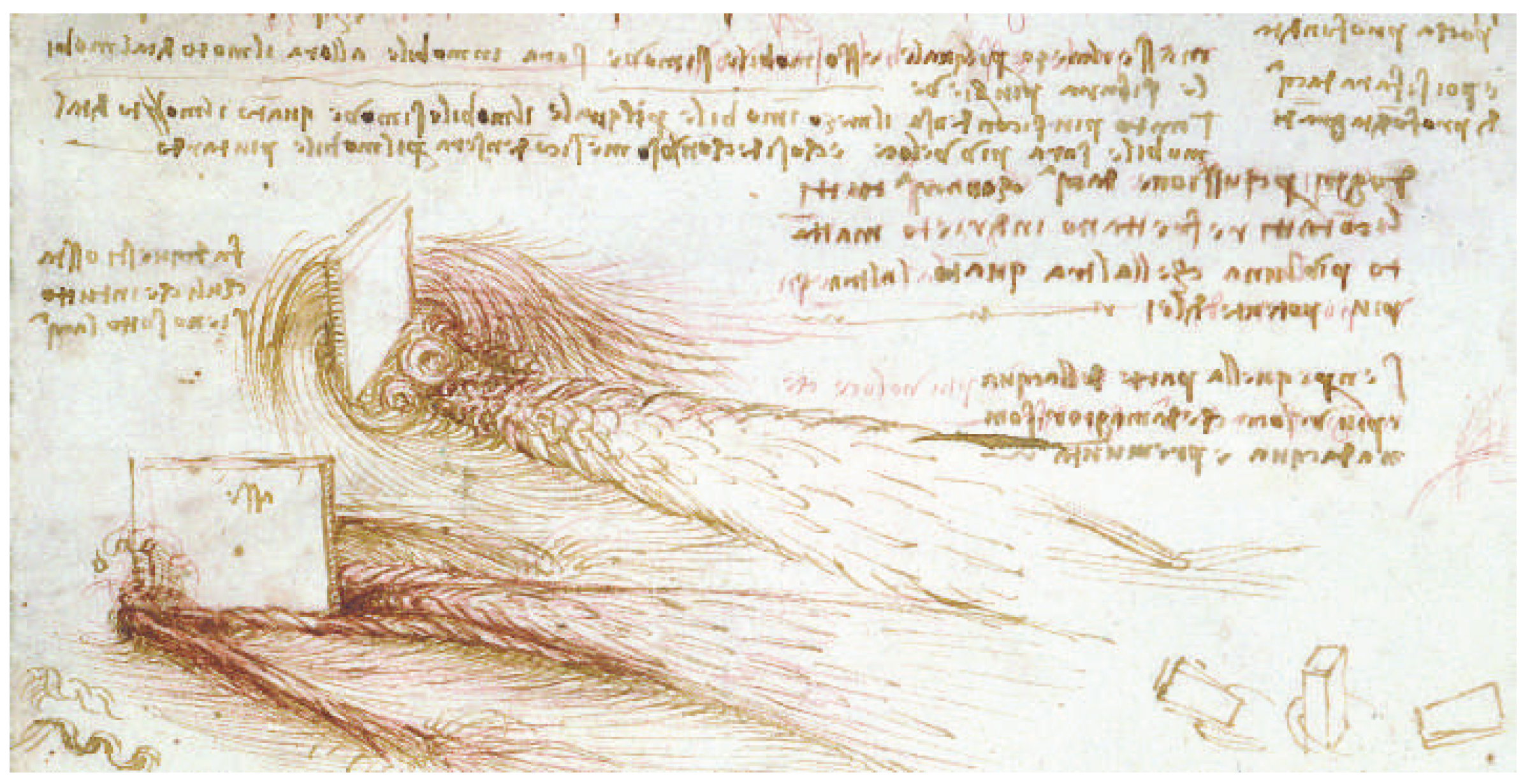
Figure 2.
Measurement of anisotropic turbulence. Structure functions of the mean positions of two beams: (A) horizontal ; (B) vertical , normalized by saturation values , , respectively. Here, is the root-mean square value of the refractive index fluctuations, L is the range, and , are constants on the order of outer scale. Reprinted with permission from Reference [32].
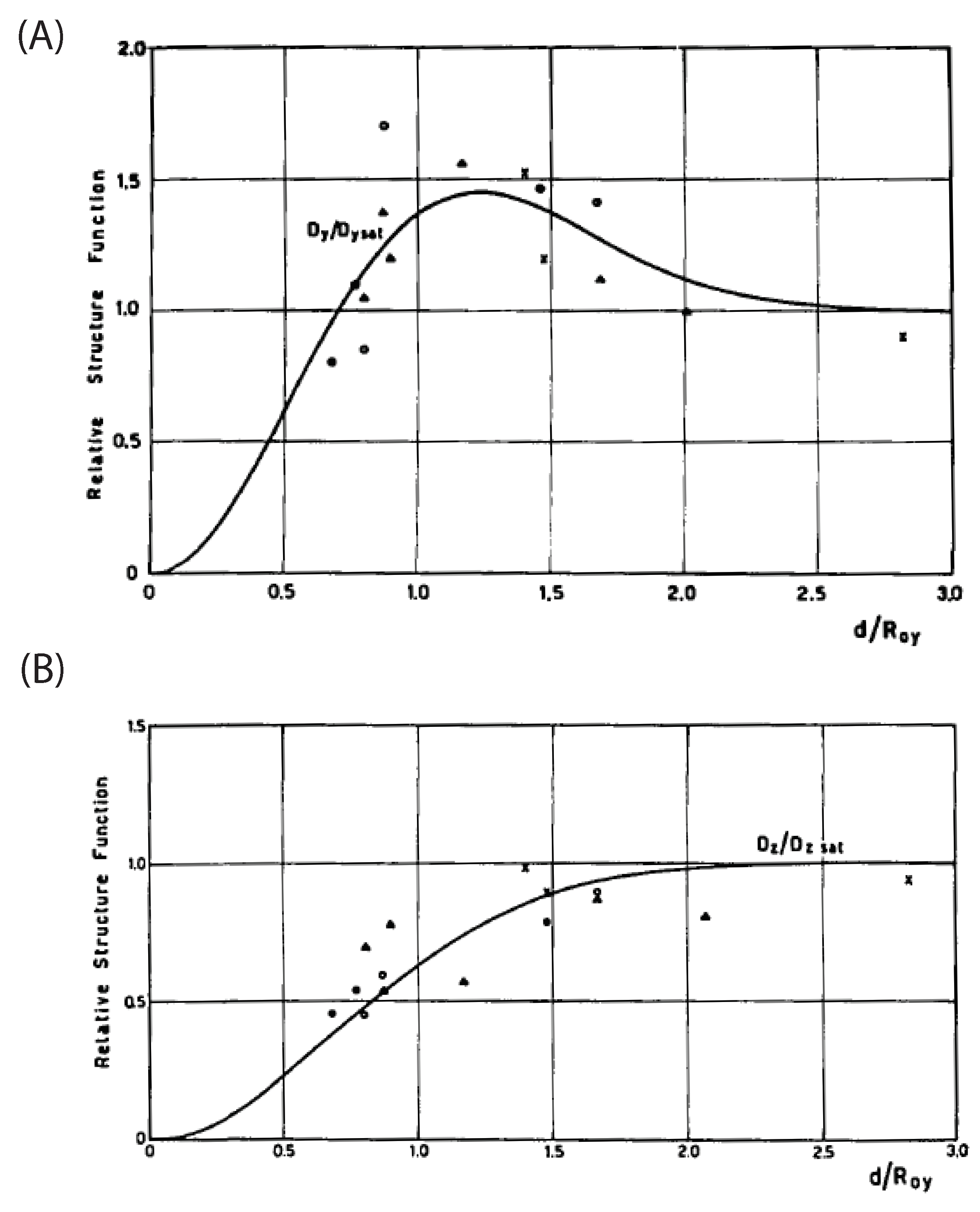
Figure 3.
Experimental campaign showing anisotropy ellipse of intensity covariance function. Top row: the same path, height from ground (a) 39 cm, (b) 84 cm, (c) 139 cm. Bottom row: at 84 cm taken over three different paths, in (a–c). Reprinted with permission from Reference [37].
Figure 3.
Experimental campaign showing anisotropy ellipse of intensity covariance function. Top row: the same path, height from ground (a) 39 cm, (b) 84 cm, (c) 139 cm. Bottom row: at 84 cm taken over three different paths, in (a–c). Reprinted with permission from Reference [37].
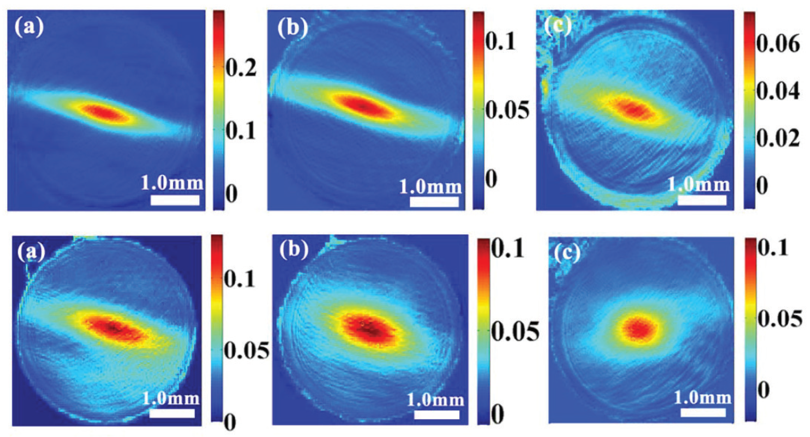
Figure 4.
Experimental field measurements compared with theoretical results showing anisotropy ellipse of intensity covariance function: (a) measurement; (b) theory; (c,d) are major and minor cross-sections (solid curves: measurement; triangles: theory). Horizontal and vertical axes in (a,b) have extent (−6 cm, 6 cm). In (c,d) horizontal axes have extent (−6 cm, 6 cm) and vertical axes are unitless with range . Reprinted with permission from Reference [38].
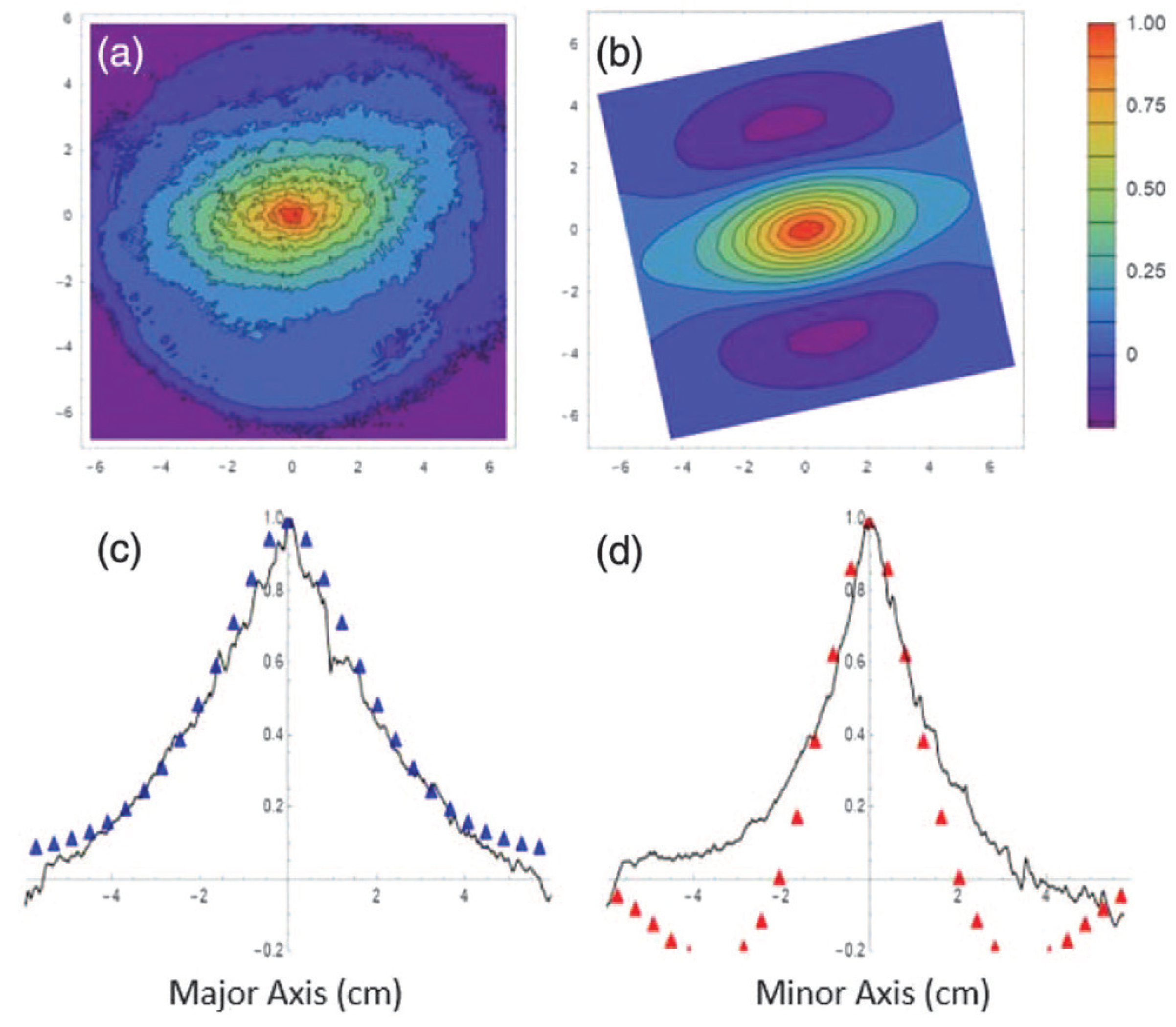
Figure 5.
The schematic diagram of a turbulator used for non-classic turbulence simulations. Reprinted with permission from Reference [48].
Figure 5.
The schematic diagram of a turbulator used for non-classic turbulence simulations. Reprinted with permission from Reference [48].
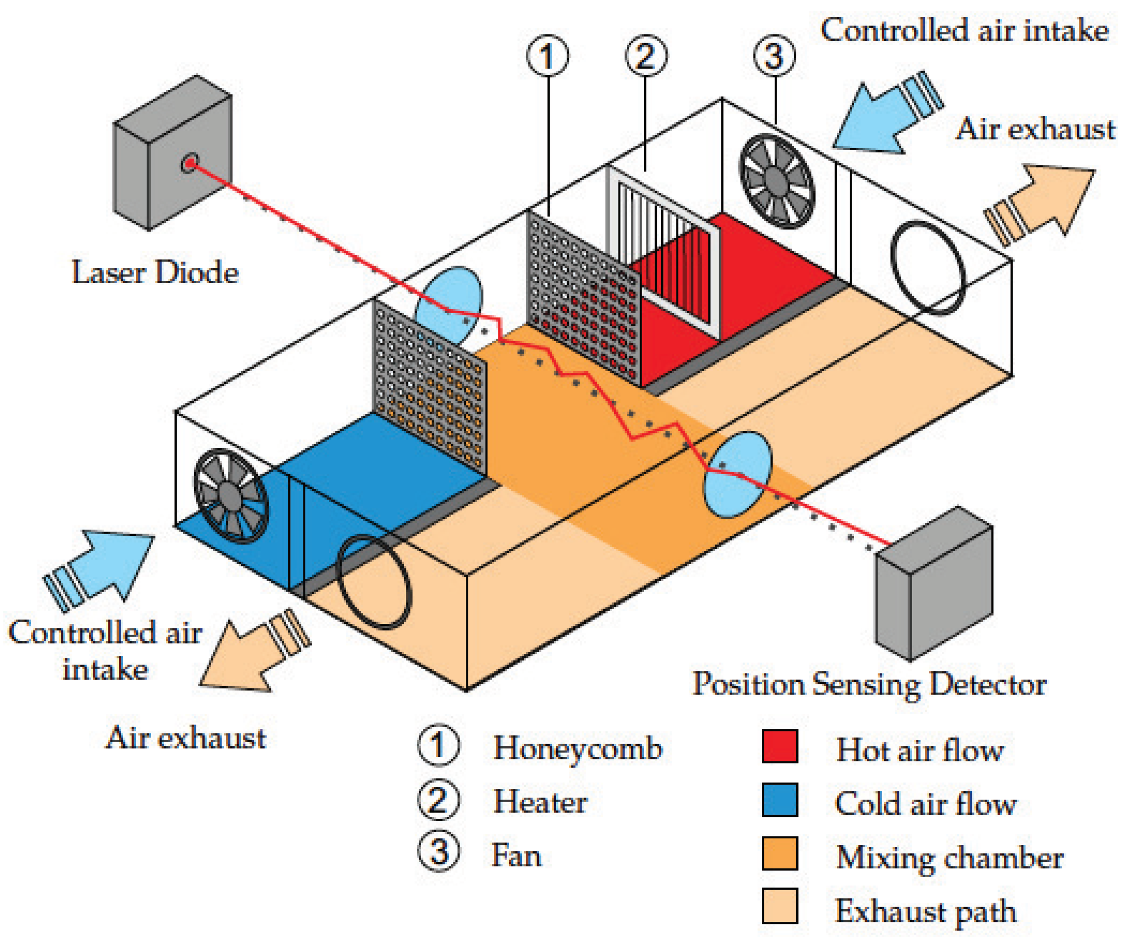
Figure 6.
Data obtained with turbulator shown in Figure 5 for unequal hot and cold air flow speeds. Reprinted with permission from Reference [48].
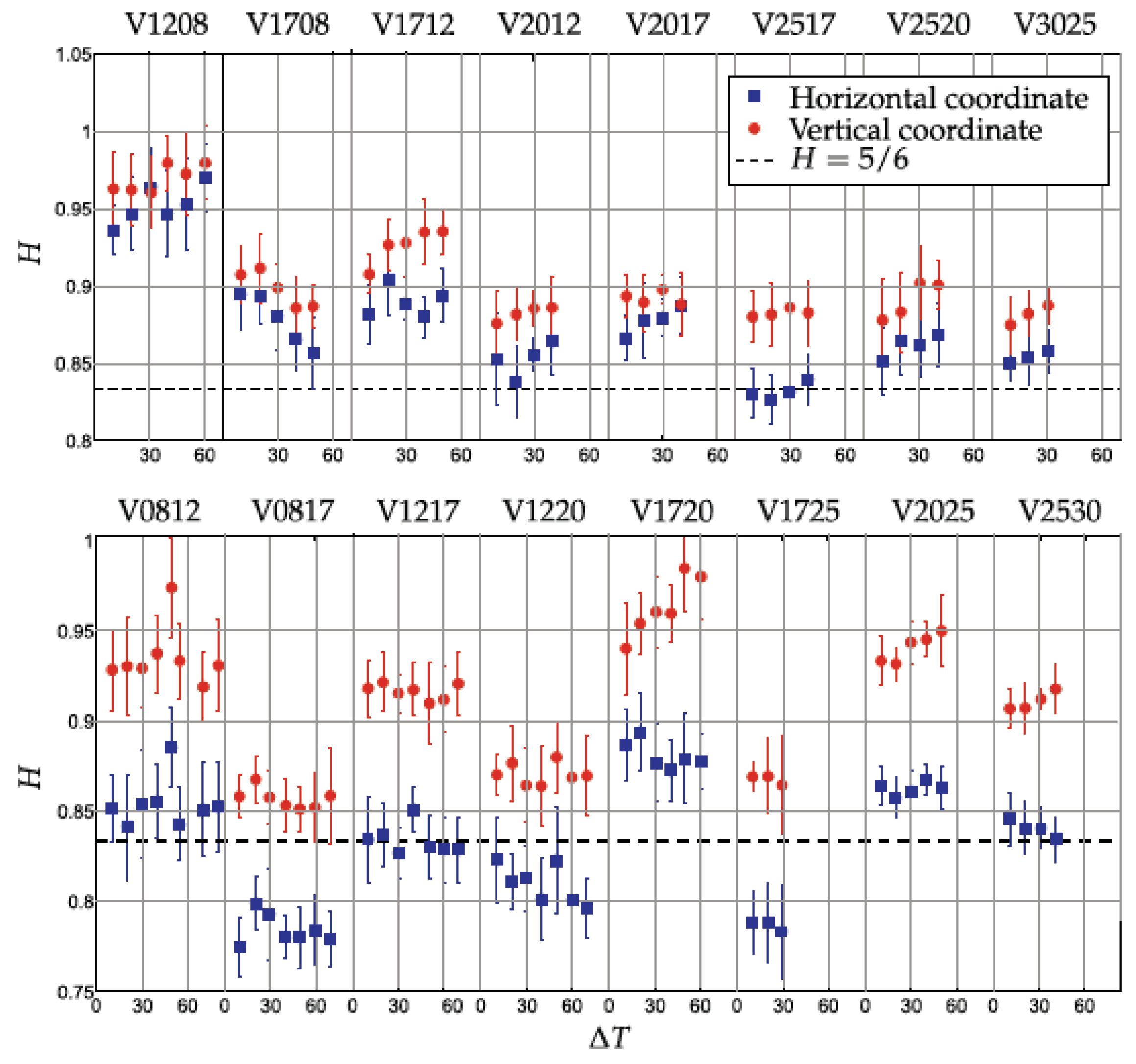
Figure 7.
Function depending on .

Figure 8.
Three-layer model of non-Kolmogorov turbulence spectrum exponent versus height z [m] above the ground. Solid curve: , ; Dashed curve: , . Reprinted with permission from Reference [62].
Figure 8.
Three-layer model of non-Kolmogorov turbulence spectrum exponent versus height z [m] above the ground. Solid curve: , ; Dashed curve: , . Reprinted with permission from Reference [62].
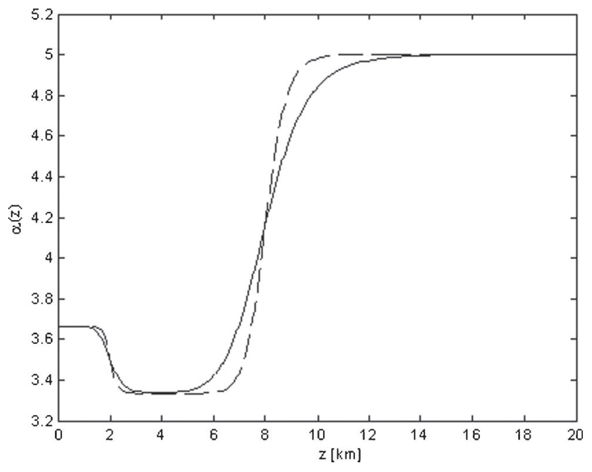
Figure 9.
Anisotropic turbulence. Vertical case. Vectors and are 2D position vectors of points in the source and in the field planes.
Figure 9.
Anisotropic turbulence. Vertical case. Vectors and are 2D position vectors of points in the source and in the field planes.
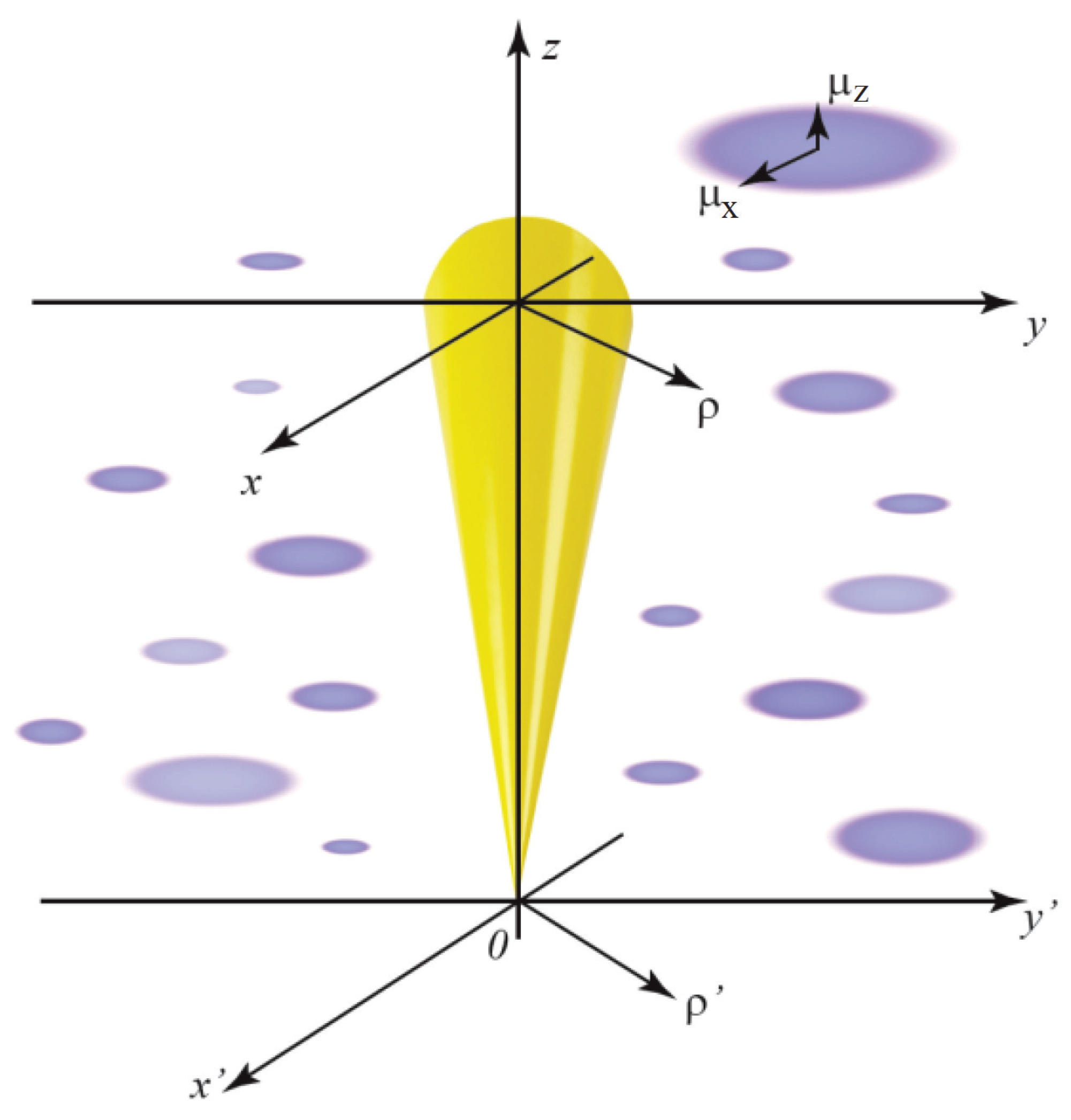
Figure 10.
Anisotropic turbulence. Horizontal case. Vectors and are 2D position vectors of points in the source and in the field planes.
Figure 10.
Anisotropic turbulence. Horizontal case. Vectors and are 2D position vectors of points in the source and in the field planes.
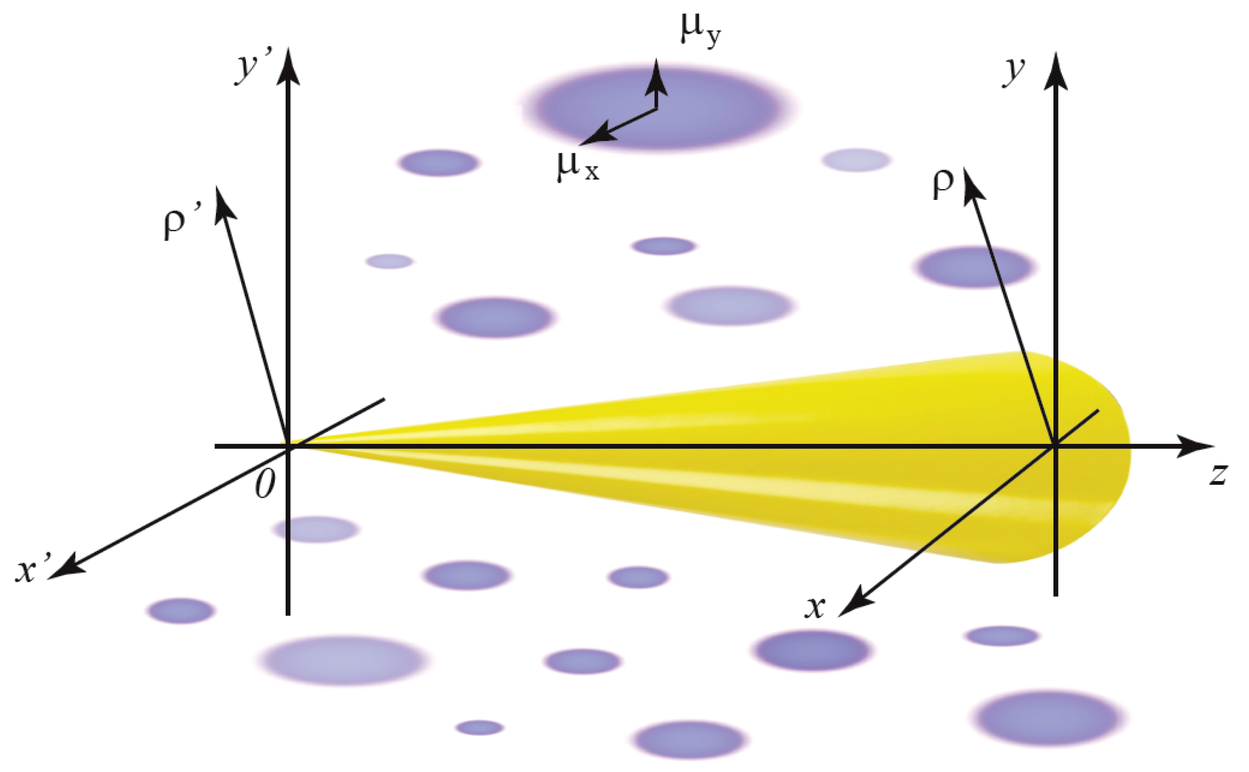
Figure 11.
Turbulent phase screens of non-classic turbulence with wrapped phase for application on SLM/DMD. Vertical turbulence with (a) , (b) . Horizontal turbulence with , , (c) , (d) . Reprinted with permission from References [81,84].

Figure 12.
The two-SLM setup for generation of any pre-modulated beam () and simulating its interaction with non-Kolmogorov turbulence (). —laser diode, —neutral density filter, L—lens, —complementary metal oxide semiconductor camera, , and are personal computers. (a–e) Generated frame-like beams passing through simulated turbulence with different ; (f) comparison of cross-sections. Printed with permission from Reference [85].

Figure 13.
The root-mean-square width of a scalar Gaussian–Schell model (GSM) beam on propagation in non-Kolmogorov turbulence. Reprinted with permission from Reference [91].
Figure 13.
The root-mean-square width of a scalar Gaussian–Schell model (GSM) beam on propagation in non-Kolmogorov turbulence. Reprinted with permission from Reference [91].
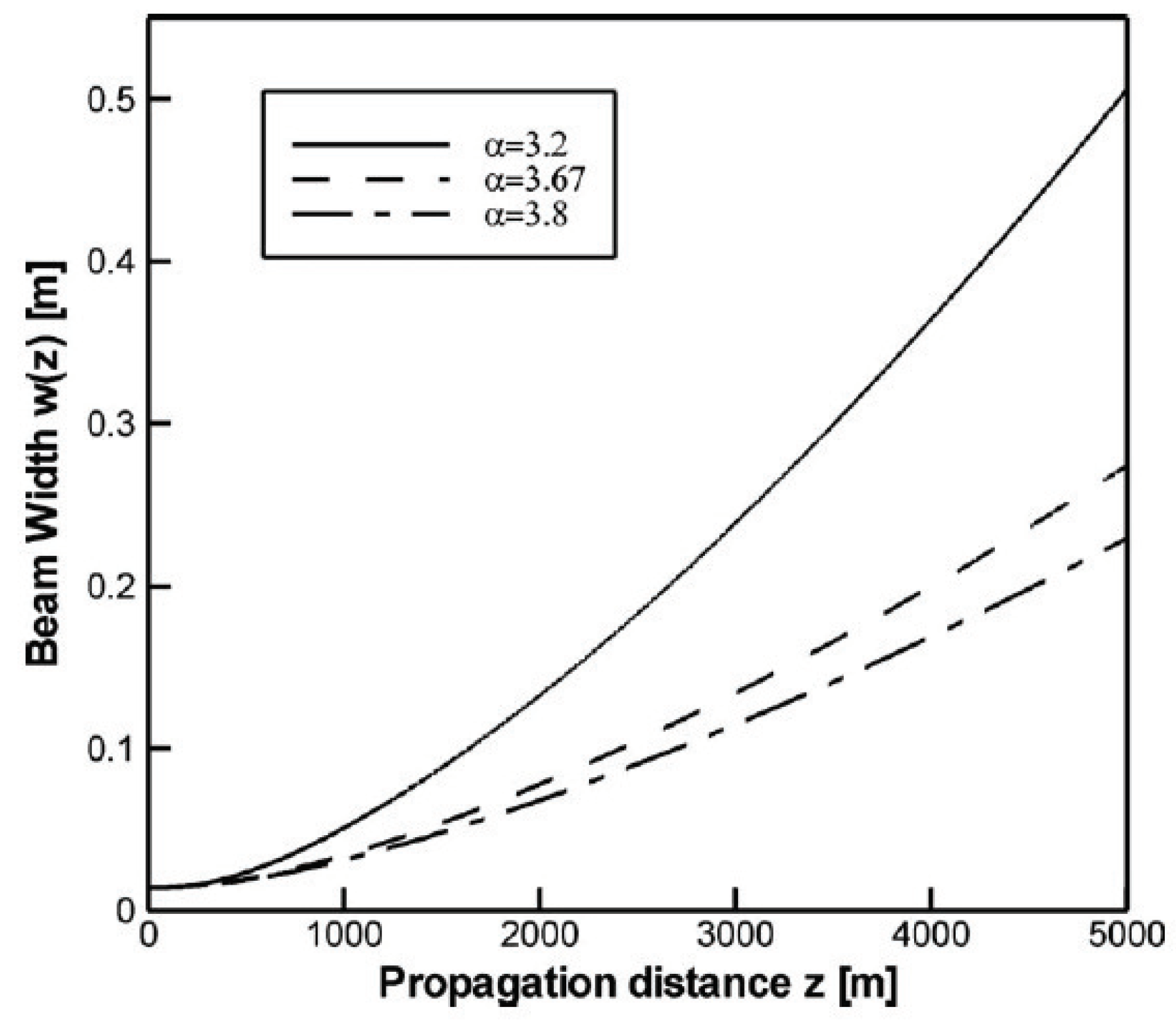
Figure 14.
Changes in (A) the degree of coherence and (B) the degree of polarization of the electromagnetic Gaussian–Schell model (EM GSM) in non-Kolmogorov turbulence. (solid curve), (dashed curve), (dotted curve) and free space (dot-dashed curve). Reprinted with permission from Reference [90].
Figure 14.
Changes in (A) the degree of coherence and (B) the degree of polarization of the electromagnetic Gaussian–Schell model (EM GSM) in non-Kolmogorov turbulence. (solid curve), (dashed curve), (dotted curve) and free space (dot-dashed curve). Reprinted with permission from Reference [90].
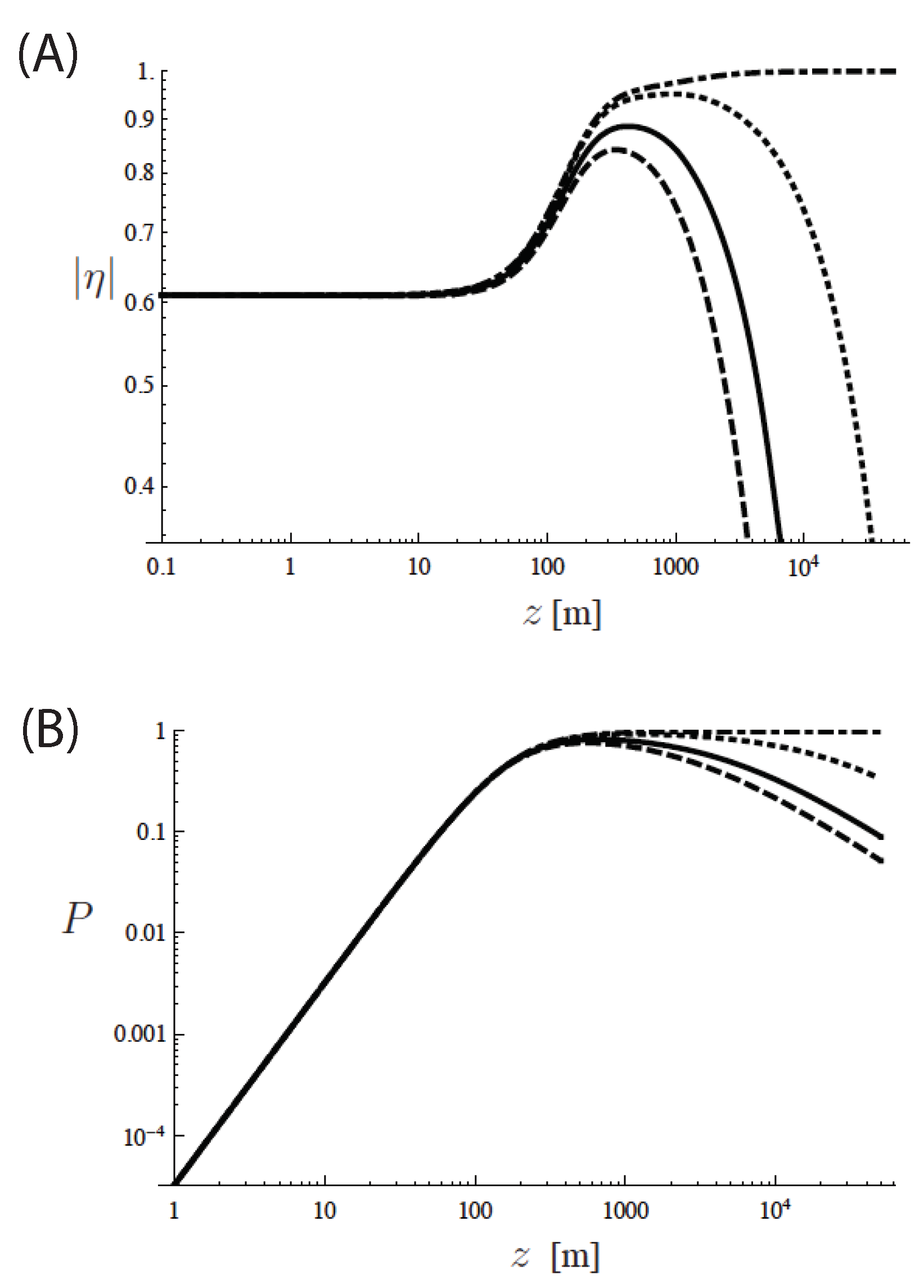
Figure 15.
Spectral density S of (A) a coherent; (B) a partially coherent electromagnetic Gaussian–Schell model (EM GSM) beam in the up-link anisotropic turbulence, for and several values of the effective anisotropic factor . Reprinted with permission from Reference [94].
Figure 15.
Spectral density S of (A) a coherent; (B) a partially coherent electromagnetic Gaussian–Schell model (EM GSM) beam in the up-link anisotropic turbulence, for and several values of the effective anisotropic factor . Reprinted with permission from Reference [94].
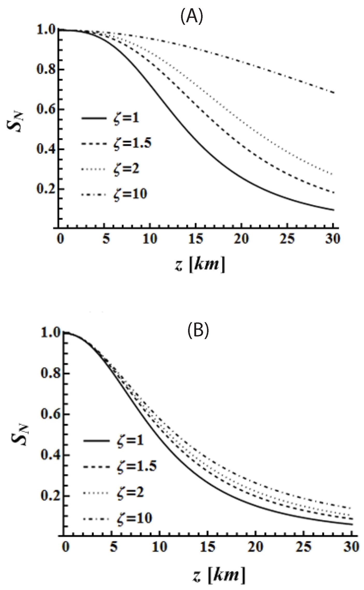
Figure 16.
Spectral density S of an electromagnetic Gaussian–Schell model (EM GSM) beam with (a–d) high; (c–h) intermediate and (i–l) low values of the typical coherence width , on propagation through an anisotropic turbulence in a horizontal direction, at specified distances. Reprinted with permission from Reference [96].

Figure 17.
Scintillation flux with fixed structure function at the Fresnel distance for six pairs of anisotropic factors along the x and y axes (shown as and in the legend). Reprinted with permission from Reference [100].
Figure 17.
Scintillation flux with fixed structure function at the Fresnel distance for six pairs of anisotropic factors along the x and y axes (shown as and in the legend). Reprinted with permission from Reference [100].

Figure 18.
Probability of fade as a function of for several cases of anisotropy and fixed structure function (shown as and in the legend). Reprinted with permission from Reference [100].
Figure 18.
Probability of fade as a function of for several cases of anisotropy and fixed structure function (shown as and in the legend). Reprinted with permission from Reference [100].

Figure 19.
Mean SNR with fixed structure function for fixed values of anisotropic factors (shown as and ). Reprinted with permission from Reference [100].
Figure 19.
Mean SNR with fixed structure function for fixed values of anisotropic factors (shown as and ). Reprinted with permission from Reference [100].
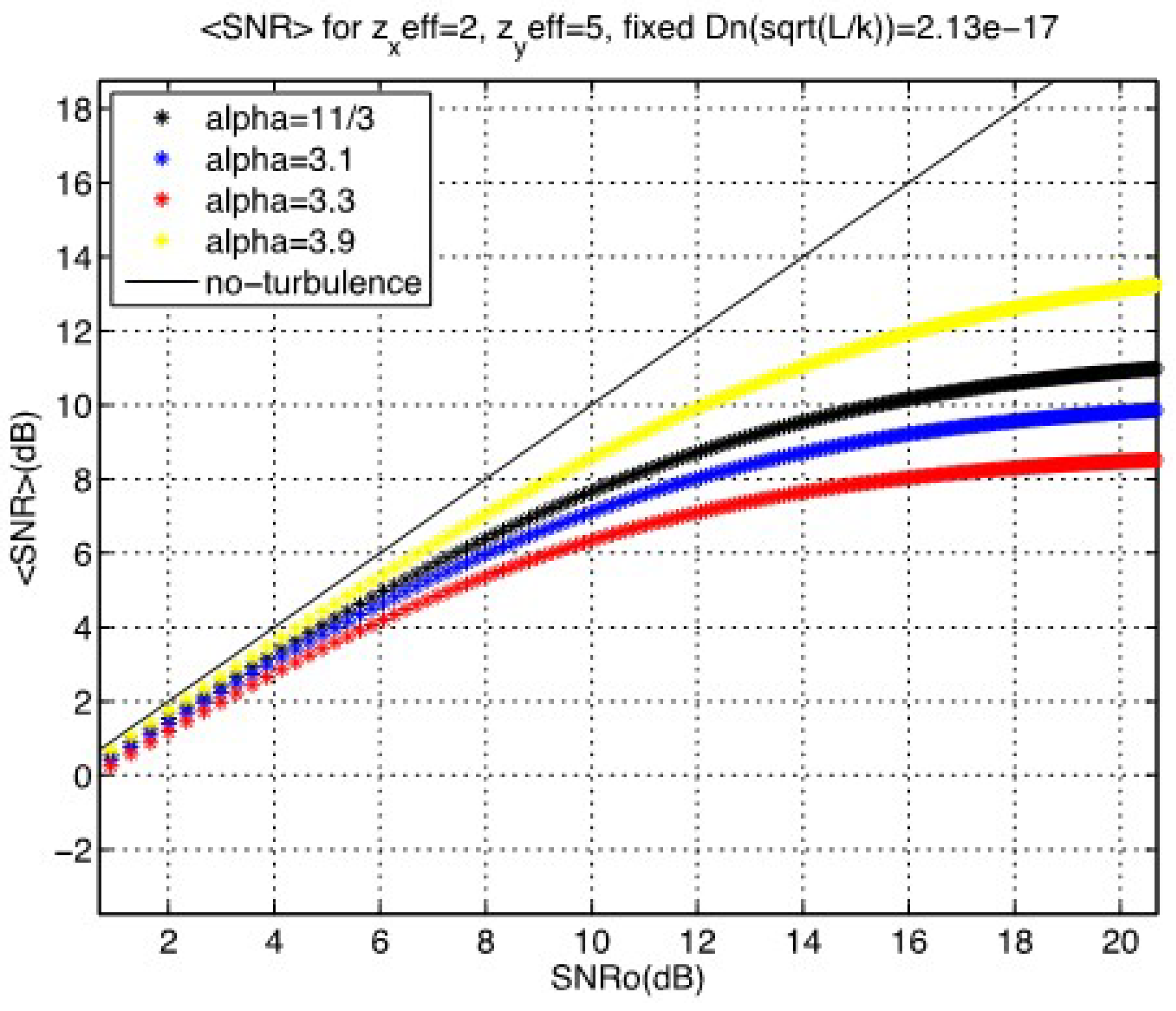
Figure 20.
Mean BER as a function of mean SNR for several sets of anisotropy factors (shown as and in the legend) with = 3.2. Reprinted with permission from Reference [100].
Figure 20.
Mean BER as a function of mean SNR for several sets of anisotropy factors (shown as and in the legend) with = 3.2. Reprinted with permission from Reference [100].
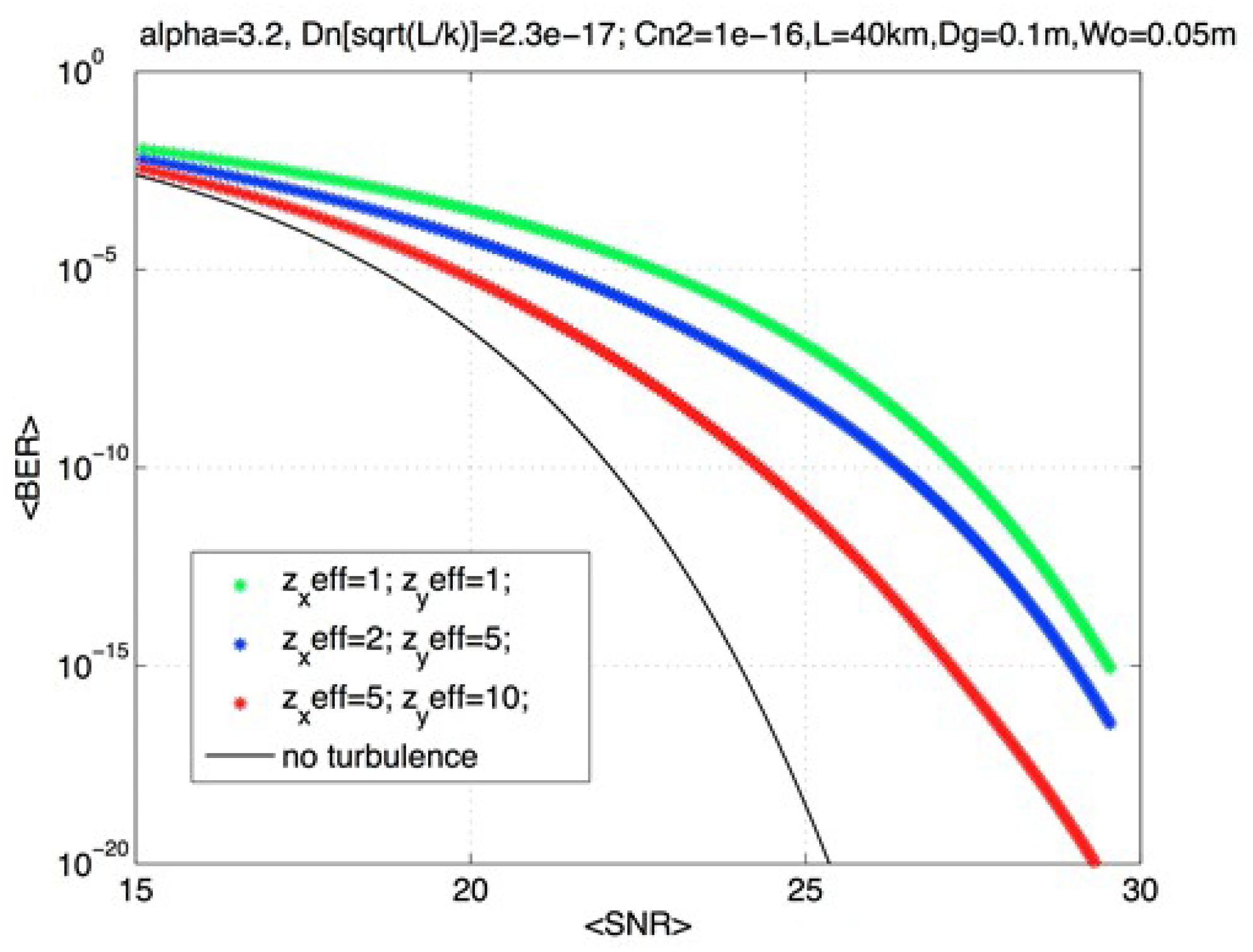
Figure 21.
Mono-static case: scintillation index as a function of the square root of the Rytov variance for several power law values. Reprinted with permission from Reference [104].
Figure 21.
Mono-static case: scintillation index as a function of the square root of the Rytov variance for several power law values. Reprinted with permission from Reference [104].
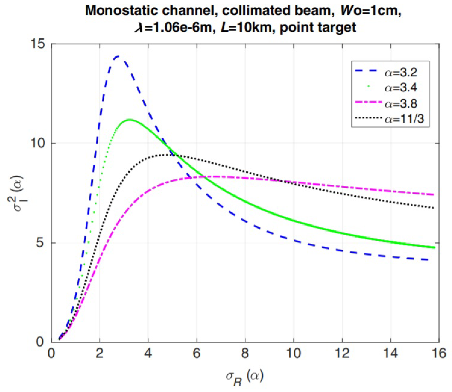
Figure 22.
Bi-static case: scintillation index as a function of the square root of the Rytov variance for several power law values. Reprinted with permission from Reference [104].
Figure 22.
Bi-static case: scintillation index as a function of the square root of the Rytov variance for several power law values. Reprinted with permission from Reference [104].

Figure 23.
Mono-static case: enhancement factor as a function of the square root of the Rytov variance for several power law values. Reprinted with permission from Reference [104].
Figure 23.
Mono-static case: enhancement factor as a function of the square root of the Rytov variance for several power law values. Reprinted with permission from Reference [104].
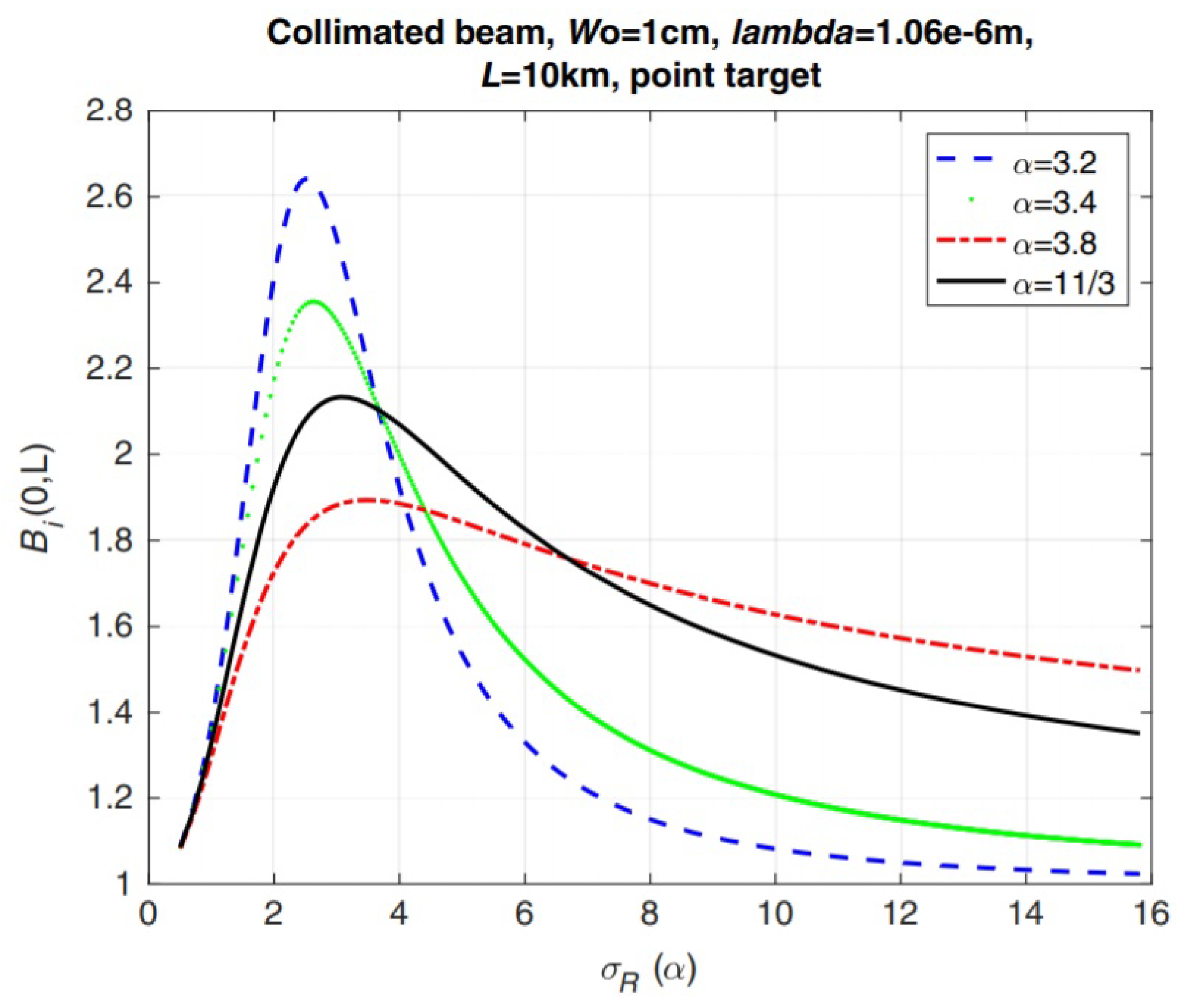
Publisher’s Note: MDPI stays neutral with regard to jurisdictional claims in published maps and institutional affiliations. |
© 2021 by the authors. Licensee MDPI, Basel, Switzerland. This article is an open access article distributed under the terms and conditions of the Creative Commons Attribution (CC BY) license (https://creativecommons.org/licenses/by/4.0/).
Share and Cite
MDPI and ACS Style
Korotkova, O.; Toselli, I. Non-Classic Atmospheric Optical Turbulence: Review. Appl. Sci. 2021, 11, 8487. https://doi.org/10.3390/app11188487
AMA Style
Korotkova O, Toselli I. Non-Classic Atmospheric Optical Turbulence: Review. Applied Sciences. 2021; 11(18):8487. https://doi.org/10.3390/app11188487
Chicago/Turabian StyleKorotkova, Olga, and Italo Toselli. 2021. "Non-Classic Atmospheric Optical Turbulence: Review" Applied Sciences 11, no. 18: 8487. https://doi.org/10.3390/app11188487
Note that from the first issue of 2016, this journal uses article numbers instead of page numbers. See further details here.