Contribution to the Understanding of Protein–Protein Interface and Ligand Binding Site Based on Hydrophobicity Distribution—Application to Ferredoxin I and II Cases

Featured Application

hydrophobicity characteristic of proteins in the sense of fuzzy oil drop model may help predict residues engaged in protein–protein and protein–ligand interaction.

Abstract

Ferredoxin I and II are proteins carrying a specific ligand—an iron-sulfur cluster—which allows transport of electrons. These two classes of ferredoxin in their monomeric and dimeric forms are the object of this work. Characteristic of hydrophobic core in both molecules is analyzed via fuzzy oil drop model (FOD) to show the specificity of their structure enabling the binding of a relatively large ligand and formation of the complex. Structures of FdI and FdII are a promising example for the discussion of influence of hydrophobicity on biological activity but also for an explanation how FOD model can be used as an initial stage adviser (or a scoring function) in the search for locations of ligand binding pockets and protein–protein interaction areas. It is shown that observation of peculiarities in the hydrophobicity distribution present in the molecule (in this case—of a ferredoxin) may provide a promising starting location for computer simulations aimed at the prediction of quaternary structure of proteins.

1. Introduction

Ferredoxins are proteinaceous electron carriers that play key physiological roles ensuring an electron flux to many essential biochemical pathways [1,2], such as—among others—steroid hormones biosynthesis in the adrenal mitochondria of vertebrates [3]. They shuttle electrons through the binding of various iron-sulfur clusters, mainly [3F4S] or [4F4S]. Other types of clusters are [3F4S] together with one [4F4S], and two [4F4S] [4,5,6,7]. Adrenodoxin is also a member of the ferredoxin family, binding the simplest polymetallic system, [2F2S] Fd, distributed in three classes: plant type, bacterial type and vertebrate type, with a structure in the core very similar [3]. Bovine adrenodoxin, for instance, is part of the mitochondrial electron transport chain responsible for the production of steroid hormones in mammals [8]. Electron transport among ferredoxins is realized by a change in the oxidation state of the iron atom, tetrahedrally coordinated with the bridging sulfur atoms in the clusters. The fold (a sheet of four strands facing two helices) is shared among members of the family [4,9]. Ferredoxin was for long associated with the fermentative chemistry of anaerobic organisms, but it is now agreed that they are ubiquitous in all domains of life, although the sequence identity is very low between the members of the family. Isoforms may have evolved not as generic electron shuttles but serve as selective couriers of valuable low potential electrons from selected electron donors to desirable electron acceptors [1].

Fuzzy oil drop (FOD) is an efficient method for the expression of a micelle-like hydrophobicity distribution in globular proteins [10]. It employs a 3D Gauss function to build a theoretical capsule (an ellipsoid) that encompasses the structure. This capsule models the shape of a globular protein in water with hydrophobic core surrounded by a hydrophilic shell but without the need for direct simulation of water molecules [11]. Such high symmetry and perfect following of this kind of distribution would render the molecule deprived of any form of biological activity except for high solubility. This phenomenon is observed in type III antifreeze proteins (AFPs). Their surface, which is covered by polar groups, opposes formation of ice crystals by affecting organization of surrounding water environment, directly contributing to survival of the cell at sub-zero temperatures [12]. Absence of exposed hydrophobic patterns drastically reduces ability of a protein to interact with other partners. A typical protein structure is however not that “perfect”. Discrepancies in the distribution of hydrophobicity, where observed status of residues (due to their pairwise interaction) does not follow the 3D Gauss-based theory (entirely or partially), are a common occurrence [13,14]. In particular, they become exceptionally apparent in amyloids [15,16]. These peculiarities, appearing along the sequence (on the so-called hydrophobicity profile), are the foundation of structural and functional analysis of proteins using the FOD model.

In this paper, we mainly discuss two ferredoxins—I (FdI) and II (FdII)—relatively small proteins (around 60 residues per chain)—with biological activity involving binding of a relatively large ligand and formation of a dimeric complex. They are a very interesting subject since they exhibit hydrophobicity distribution that is among the best in terms of accordance with 3D Gauss function we encountered so far, even stronger when compared to the aforementioned type III AFPs. Yet in contradiction to what FOD model would expect from them, these ferredoxins form complexes while AFPs do not. This warrants their more thorough investigation.

Theoretical distribution of hydrophobicity (3D Gauss-based), when confronted with observed (empirical) status within FdI and FdII molecules, reveals that even with such strong global-scale accordance, there are fine details (single residues located on the hydrophobicity density map) that carry information which can be linked to the protein–ligand (P-L) and protein–protein (P-P) interaction areas and may be used to—at least partially—unveil them. We also show here that a type III AFP does not exhibit the same phenomenon, which is in line with its biological function. This suggests that FOD-based analysis could be another metric in the process of prediction of ligand binding cavities or quaternary structure of proteins when tertiary structure is available [17]. It is the main goal of the ongoing experiment at CAPRI [18,19]. A revised contact exploration and prediction protocol is presented in this paper. To display its capabilities, we also apply it to a counterexample protein: a non-globular dimer deprived of stable hydrophobic core.

2. Materials and Methods

2.1. Data

We selected two ferredoxin structures (FdI and FdII) from the Protein Data Bank (PDB) [20,21]. Biological assemblies of these proteins are homodimeric (as assigned by their authors) with cyclic complex symmetry. Both molecules belong to the same CATH homologous superfamily 3.30.70.20 [22,23], the alpha-beta plaits.

We also accessed two other PDB structures for comparative analysis in Section 3.8: a globular, monomeric type III antifreeze protein and a symmetric, homodimeric complex of Rad50 domains from Mre11—helix hairpins involved in chromosomal maintenance.

Basic information of all four molecules summarized in

Table 1. Protein structures under consideration.

Protein	PDB Code	Organism	Quaternary Structure	Chain Length	Ligand	CATH Domain	Ref.
Ferredoxin I (FdI)	1FXR	Desulfovibrio africanus	homodimer, symmetric	64 aa	[4F4S]	3.30.70.20	[24]
Ferredoxin II (FdII)	1FXD	Desulfovibrio gigas		58 aa	[3F4S]		[25]
Antifreeze type III (AFP)	9MSI	Macrozoarces americanus	monomer	66 aa	none	3.90.1210.10	[26]
Rad50 domain (Mre11 complex)	1L8D	Pyrococcus furiosus	homodimer, symmetric	103 aa	Hg2+	1.10.287.510	[27]

while their 3D presentation is available in Figure 1.

The structure of Ferredoxin I (FdI, PDB code: 1FXR [24], Figure 1a) is a homodimer with 64 amino acids and one [4F4S] cluster in each chain. These ligands are located in pockets located at opposite sides of the symmetric complex. Each ligand interacts with 11 residues from the chain, detected in accordance with PDBsum atom distance criterion for non-bonded contacts [28,29] (two residues are assumed to be in contact if there is at least one pair of non-hydrogen atoms—one from each residue—with Euclidean distance not greater than 3.9 Å). Among these residues are four cysteines (C11, C14, C17 and C54), experimentally determined to coordinate the iron-sulfur cluster.

The structure of Ferredoxin II (FdII, PDB code: 1FXD [25], Figure 1b) is a 58 amino acid monomer, although it is isolated as a tetramer (according to Kissinger et al., “there are four molecules in the unit cell, but it is apparent from an examination of the crystal packing interactions that their arrangement is unlikely to be relevant to tetramer formation” [25]). PDB file data of 1FXD provides symmetry operators in REMARK 350, application of which results in a perfectly symmetric homodimeric complex. A single [3F4S] cluster is present in each chain, involved in non-bonded contacts with 10 residues. Ligand coordination is handled by C8, C14 and C50. The fact that FdI is bound to the cluster by four cysteines, and FdII by three, has already been described [9].

The structure of type III antifreeze protein (PDB code: 9MSI [26], Figure 1c) is a 66 amino acid monomer with no partner molecules present along its structure.

The structure of Rad50 domain (PDB code: 1L8D [27], Figure 1d) is a component of the Mre11-Rad50-Nbs1 complex, which plays role in several DNA-related processes. Unlike the other three proteins presented here, it assumes the form of a long coiled coil, limited in the PDB file to the neighborhood of a hook-shaped region in the middle of its sequence. Pfam [30] domain segment for this structure is 423–474 (coiled-coil zn hook). Hopfner et al. inform that Rad50 forms dimeric complexes through coordination of a zinc ion by four conserved cysteines (two per chain) located in this hook [27]. 1L8D PDB file contains however a substituted Hg²⁺ ion which allowed to obtain the same structure in better resolution. The whole complex works as a M2R2 tetramer or (M2R2)₂ octamer.

2.2. FOD Model

Fuzzy oil drop (FOD) model has been described in detail in [31,32,33], hence only its key features are reminded in this paper (with example figures in the Supplementary Materials).

FOD requires tertiary structure of a protein as the source for its calculation. The results of this calculation are two “main” hydrophobicity distributions:

• O—observed hydrophobicity distribution based on pairwise hydrophobic interactions between residues, calculated using Michael Levitt’s polynomial [34];
• T—theoretical hydrophobicity distribution calculated using 3D Gauss capsule fit to the molecule (Figure S1), based on location of residues in respect to this “drop”.

An i-th residue in the sequence (of length N) is assigned two values: T_i and O_i. The protein is then analyzed on the basis of comparison between these T and O distributions. A perfectly soluble molecule would have T ≡ O (T_i = O_i for all i between 1 and N), but it is the differences between those distributions that reveal the structural and functional properties as seen from the perspective of hydrophobic core formation [35].

Since T and O are normalized to enable their comparison, differences between them are measured using Kullback–Leibler divergence entropy (D_KL) [36]. The result of this comparison is called the RD coefficient (relative distance) which expresses the T vs. O “distance” on a scale between 0 and 1 (Figure S2). The closer the value of RD is to 0, the higher accordance between T and O is registered, with 0 meaning that T ≡ O. On the other hand, value of RD closer to 1 denotes higher discordance.

Use of RD as a measure is possible due to introduction of R (“random”)—a distribution opposite to 3D Gauss function, representing situation where all residues have uniform hydrophobicity regardless of their location or their amino acid (R_i = 1/N for all i between 1 and N), with RD = 1 meaning that O ≡ R. RD = 0.5 is therefore the accordance vs. discordance threshold, marking a tipping point between observation of the development of a stable hydrophobic core and the lack of such stability.

T, O and R hydrophobicity profiles (and subsequently the RD value binding them together) can be calculated for any structural unit, typically a chain, domain or complex, but also for helices, sheets or for any number of residues (in sequence or scattered), as long as all T_i and all O_i are above 0. In each of these cases, the 3D Gauss capsule (the “drop” ellipsoid) is fitted to the effective atoms of selected residues.

Once T, O and R profiles are obtained for the input structure, RD can also be used to analyze its sub-domain fragments. This is useful to determine the status of a specific part in respect to the whole, for example a sheet in the chain or a chain in the complex. By calculating RD only for an extracted subset of T, O and R distribution values, one can express the participation of this selection in stability of the hydrophobic core [37].

There is also a fourth distribution—H—which denotes the (also) normalized intrinsic hydrophobicity of residues. It is based purely on their amino acid and matching value of hydrophobicity parameter (H parameter in short), acquired by default from the FOD hydrophobicity scale (0.0 < KEDQRNPSTGAHYLVMWIFC ≤ 1.0). Calculation of H is, actually, necessary to obtain O. It is used for hydrophobicity-based analysis from the sequence perspective, which is especially useful in the case of amyloids [38].

In addition to RD, correlation coefficients (CC) can be calculated to express another type of relation between T, O and H, yielding three normalized values labeled HvT, TvO and HvO (i.e., TvO is the correlation coefficient of T vs. O). This comparison helps with identification of the dominating tendency in hydrophobic core generation.

It should be noted here that the notion of hydrophobic core in the context of fuzzy oil drop model is tightly coupled with the presence of polar surface shell that surrounds and shields it from water environment. These two components “drive” the molecule towards a structure that corresponds to the idealized hydrophobicity distribution [39].

Finally, it should also be mentioned that T and O comparison can be employed in the context of analysis and search for residues engaged in ligand binding [40] and in protein–protein interaction [41]. Such residues should exhibit discordant status with the model (high difference between distributions): excess of hydrophobicity on the surface of the molecule (P-P patch) or a localized deficiency towards the center (P-L pocket). A modified detection algorithm employing this principle is described in Section 3.6 with thorough explanation and examples. It is applied to all four proteins from Table 1.

2.3. MIR Model

MIR model (briefly described here) can be regarded as a prediction of peaks in the distribution of hydrophobic residues along the sequence, because it is not randomly distributed. By hydrophobic we mean any residue from this list: F, I, L, M, V, W and Y. A simulation of the folding process is performed by means of successive random displacements of the alpha carbons of the protein chain, initially randomly distributed at the nodes of a grid, with the constraint of respecting the constant distance between two residues neighbors along the sequence [42]. At each trial of a new conformation corresponding to the displacement of one alpha carbon to an empty node of the lattice, Metropolis criterion is used to decide rejection or acceptation of the new conformation. Periodically, the number of neighbors non-covalently linked (NCNs) is recorded for each amino acid along the chain. At the end of the simulation this number is smoothed, and the local maxima in this distribution are called smoothed most interacting residues (SMIRs). We previously showed that they capture, at some medium resolution, the distribution of hydrophobicity along the peptide chain that is at the principle of secondary structure formation [43].

We already compared FOD and MIR approaches on the immunoglobulin and flavodoxin folds [44]. When several structures are available, a very limited number of positions are both SMIR and in agreement with the FOD model. It was shown for these two folds that these specific positions are, actually, the folding nucleus, i.e., the first set of amino acids which mutual interaction is compulsory for the folding of the chain.

2.4. Tools and Websites

Images of the protein structures were rendered with PyMOL [45,46]. Charts were plotted using Matplotlib library [47]. FOD results were calculated using state-of-the-art open-source Python libraries for scientific computation [48,49]. Sequence and structure similarity measurements were carried out on Matras server [50,51]. Solvent-accessible surfaces were resolved using MSMS program [52,53].

Online calculation of fuzzy oil drop hydrophobicity profiles and related data is available at http://fod.cm-uj.krakow.pl web server. MIR and SMIR data was downloaded from the SPROUTS web server at http://sprouts.rpbs.univ-paris-diderot.fr.

3. Results

Sequence similarities between FdI and FdII, their structural features (including complex formation) and hydrophobicity profiles eventually leading to prediction of non-bonded interactions are the object of this work. We start from the sequence, then move to the structure (of monomers and dimers) to finalize with presentation how a “seed” for the search for residues engaged in P-L and P-P interaction can be found in these two ferredoxins through the evaluation of hydrophobicity density map (Section 3.6 and Section 3.7). Results of comparative analysis and simulation for type III AFP and Rad50 are presented in Section 3.8. Hydrophobicity-based analysis was performed by the means of FOD model with the support of MIR model.

3.1. Sequence Analysis

To measure the sequence and structure similarities between FdI and FdII, their PDB structures were submitted to Matras server, which is known to be among the best tools for 3D structure alignment [54,55].

Based on data received from Matras, sequence similarity between FdI and FdII is measured at 41.4% after the introduction of six insertions in the shorter sequence (FdII): one between N5 and D6, one between D37 and S38 and two padding residues at each chain terminus. This alignment, as well as the secondary structure composition and non-bonded contacts is presented in Figure 2. Secondary structure similarity between FdI and FdII is determined to be 91.4%, with 100% of beta sheet match.

FOD model takes hydrophobicity as the most important characteristic of amino acid sequence during structure formation. Due to sequence and structure similarities between FdI and FdII, a comparison of their intrinsic hydrophobicity (H) is relevant. Their H parameter profiles can be visually compared in Figure 2 and Figure 3.

In all, 25 out of 64 residues in the aligned sequences match exactly (same amino acid), while 16 from the rest have similar value of H parameter—no more than 0.2 difference (20% when measured on FOD hydrophobicity scale—between 0 and 1). Moreover, 10 out of those 25 matching residues inhabit the two helical regions present in both proteins.

FdI vs. FdII H parameter correlation coefficient—with six residues omitted due to insertions—is equal to 0.67. There are however nine outliers (Figure 3), determined as pairs of residues with H parameter difference higher than 0.4 (40% of the length of FOD hydrophobicity scale). These are: Y5-E3, A21-C18, A26-E23, K37-I34, V39-P36, Q44-L40, E46-C42, C58-A54 and W61-R57 (first residue from FdI, second residue from FdII). Elimination of those outliers increases the correlation coefficient to 0.92. This suggests rather high similarity of intrinsic hydrophobicity distribution along the two chains.

On Figure 2 and Figure 3 one can see that almost all residues engaged in P-P interaction (apart from E46 from FdI) are located in the loop regions. Residues in the vicinity of the ligand are also mostly outside the secondary structure or—with the sole exception of C17-C14 pair—they stay at extremities of helices and strands. Ligands appear to be located in mostly H-wise hydrophobic pockets (11–17 and 54–59 in FdI numbers), while the other unstructured fragments (7–10, 28–32 and 37–42 in FdI numbers) exhibit mostly non-hydrophobic status. That is where protein–protein interacting residues are located. The exceptions are: M24 and V32 in FdII and V39 surrounded by P-P contacts in FdI.

This above situation is interesting because it seems to contradict the expectations of FOD model. An example where hydrophobicity plays a significant role in quaternary structure formation are monomers with exposed significant hydrophobic patches (causing core instability) that become shielded from the solvent in complex. Same principle, but with reversed logic applies to ligand binding. Presence of a pocket introduces space unoccupied by atoms, which causes drop of hydrophobicity within the body of the protein. Ferredoxins appear to not conform to either of these phenomena.

While FOD does not try to undermine the prevailing dogma that information about protein structure is encoded in its sequence, it promotes importance of external factors [56], hence the need for structure analysis and a more detailed hydrophobicity-based investigation. An investigation that takes into account the influence of solvent on the molecule. Such information is carried by the T and O hydrophobicity profiles.

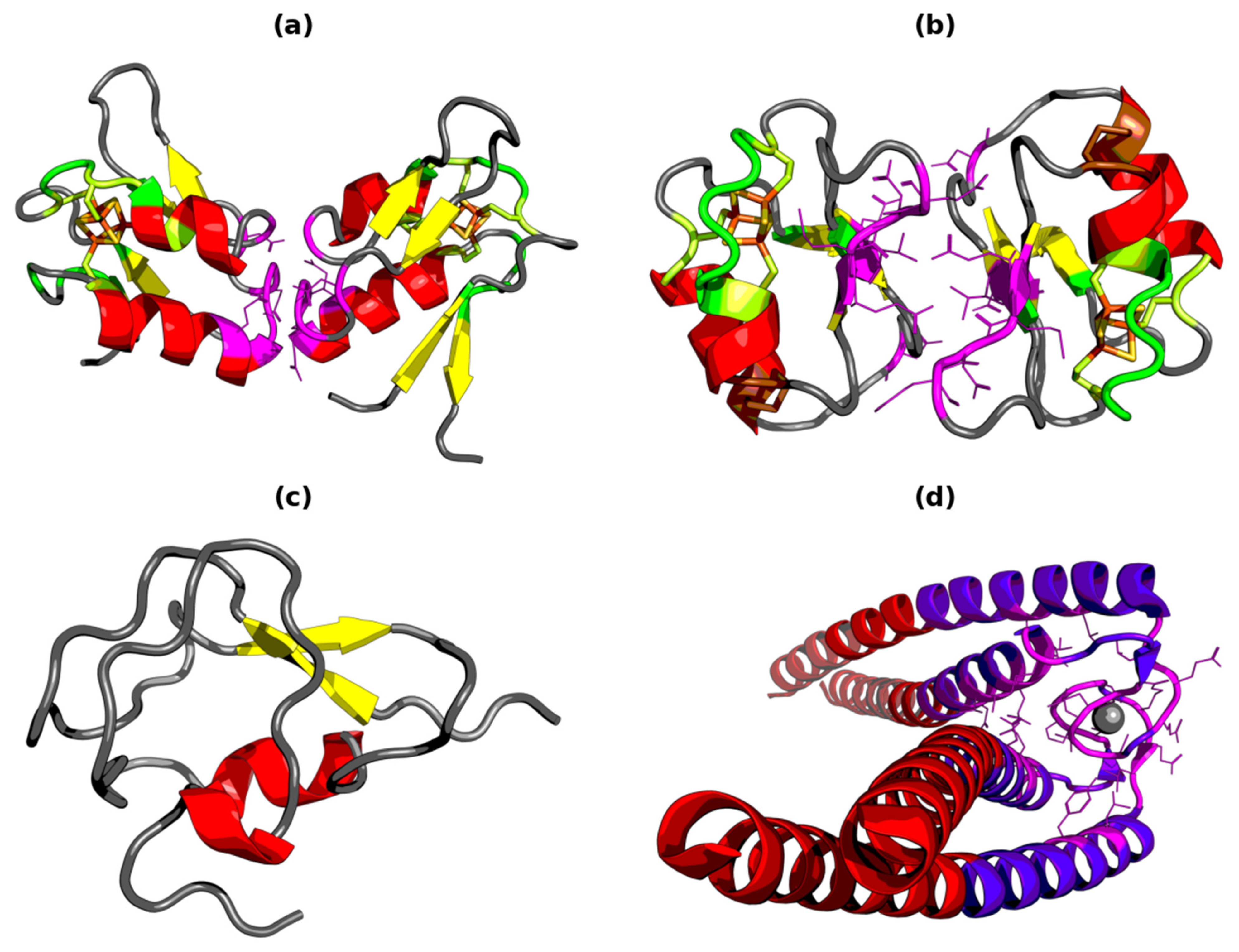
3.2. Structure Analysis

Monomers of FdI and FdII were superposed in PyMOL using CE algorithm [57] (cealign function of the program), which resulted in RMSD of 1.75 Å over 56 residues. This superposition is shown in Figure S3a. Given their same CATH assignment and almost-identical secondary structure, this is not surprising. Due to REMARK 350, chains of FdII are truly identical, but there is a little bit of difference between the chains of FdI, caused by their outlying termini. Chain A vs. chain B cealign RMSD is 0.98 Å for complete chains but drops to 0.21 Å when the two residues at each terminus are ignored.

When dimers are compared (Figure S3b)—when the other two chains are added back to the superposed monomers—it becomes clear that complex formation happens very much differently between the molecules. In FdI the protein–protein interface (seven residues: G23, D38, E40, G41, A42, S43 and E46) forms an “extension” in the helical segment direction, while in FdII, the two chains face each other somewhat with their beta sheets (also seven residues: E3, E23, M24, N25, E26, V32 and D37). The only common member is the G23-E23 pair. P-P interface in FdI is also more compact—relatively small compared to the whole protein but forming a straight “wall” with no sidechains protruding significantly into the inter-chain space. In FdII however the interface is assuming a more distributed formation: there are six residues located at one side and a lonely E3 on the other side of a crevice that can be found close to the axis of rotation of the complex.

Iron-sulfur clusters are bound in pockets located spatially in the same location in each monomer (Figure S3a). Residues interacting with them are also roughly the same in terms of numbers: V6, C11, I12, A13, C14, E15, C17, C54, V56, C58 and I59 in FdI and C8, M9, A10, C11, E12, A13, C14, A31, C50 and I55 in FdII, with the main sequence segments (containing three and two cluster-coordinating cysteines, respectively) being C11-C17 in FdI and C8-C14 in FdII. These segments match each other perfectly in terms of secondary structure once the sequences are aligned (Figure 2). A match is also found in terms of hydrophobicity: five residues belonging to each pocket are identical, while the remaining two pairs (I12-M9 and S16-A13) have similar H parameter values.

The other two cysteines in FdII that are not engaged in the interaction with the ligand (C18 and C42) form a disulfide bond instead. They join ends of helices at the other side of the protein, located in opposite direction to the binding pocket.

Calculation of solvent-accessible surfaces informs that A34 and V47 in FdI and V43 in FdII are the only residues unfeasible for non-bonded contacts with other molecules (no surface vertex within 3.9 Å range of any of their atoms).

3.3. Hydrophobicity Characteristic—Monomers

The status of monomers of FdI and FdII and their selected fragments (ordered secondary structure and residues engaged in P-P interaction and ligand binding) is given in

Table 2. Hydrophobicity status of monomers of FdI (1FXR) and FdII (1FXD) and their selected fragments.

Fragment	Residues		RD		TvH		OvT		OvH
	FdI	FdII	FdI	FdII	FdI	FdII	FdI	FdII	FdI	FdII
monomer	chain A	chain A	0.33	0.27	0.56	0.60	0.72	0.78	0.79	0.86
strand A.1	3–6	1–4	0.18	0.25	0.91	0.70	0.98	0.86	0.86	0.97
strand A.2	59–62	55–58	0.19	0.15	0.82	0.79	0.99	0.95	0.76	0.93
sheet A	strand A.1 + A.2	strand A.1 + A.2	0.21	0.18	0.83	0.69	0.94	0.91	0.77	0.87
strand B.1	25–27	22–24	0.04	0.18	0.46	0.71	1.00	0.97	0.49	0.86
strand B.2	34–36	31–33	0.83	0.89	−0.48	−1.00	0.84	−0.99	−0.88	0.99
sheet B	strand B.1 + B.2	strand B.1 + B.2	0.32	0.26	0.20	0.53	0.73	0.83	0.45	0.86
all sheets	sheet A + B	sheet A + B	0.23	0.19	0.73	0.64	0.90	0.90	0.71	0.84
no sheets	!(sheet A + B)	!(sheet A + B)	0.33	0.26	0.45	0.57	0.72	0.81	0.80	0.87
helix 1	15–21	13–17	0.23	0.18	0.85	0.81	0.97	0.94	0.88	0.96
helix 2	43–54	41–49	0.35	0.28	0.59	0.70	0.71	0.82	0.93	0.92
all helices	helix 1 + 2	helix 1 + 2	0.31	0.25	0.70	0.76	0.81	0.88	0.90	0.94
no helices	!(helix 1 + 2)	!(helix 1 + 2)	0.34	0.29	0.55	0.56	0.70	0.74	0.74	0.84
P-P	FdI(P-P)	FdII(P-P)	0.46	0.18	0.24	0.65	0.33	0.87	0.92	0.91
no P-P	!(FdI(P-P))	!(FdI(P-P))	0.31	0.28	0.56	0.59	0.75	0.77	0.79	0.85
P-L	FdI(P-L)	FdII(P-L)	0.40	0.45	0.37	0.07	0.67	0.63	0.84	0.69
no P-L	!(FdI(P-L))	!(FdII(P-L))	0.30	0.27	0.62	0.66	0.75	0.79	0.73	0.87
catalytic	11,14,17,54	8,14,50	0.25	0.27	n/a	n/a	0.90	0.92	n/a	n/a
no catalytic	!(11,14,17,54)	!(8,14,50)	0.33	0.28	0.58	0.59	0.72	0.77	0.76	0.85
S-S bond	n/a	18–42	n/a	0.25	n/a	0.62	n/a	0.78	n/a	0.90
no S-S bond	n/a	!(18–42)	n/a	0.30	n/a	0.58	n/a	0.78	n/a	0.83

Note: P-P denotes residues engaged in protein–protein interaction. P-L denotes residues engaged in ligand binding. “Catalytic” denotes ligand-coordinating cysteines. S-S bond denotes chain segment between residues forming the disulfide bond. “No” before name of a fragment and an exclamation mark around data in Residues column means that RD and correlation coefficients (TvH, OvT and OvH) were obtained for all residues except those presented in Residues column (i.e., everything except P-P contacts). Values given in bold distinguish status of accordance with the model (RD < 0.5). Underlined values exhibit correlation coefficient difference between the proteins higher than 0.5. TvH and OvH are unavailable for catalytic residues due to all of them having same H value (all cysteines).

. T and O hydrophobicity density profiles are shown in Figure 4. Profiles for FdII have two modes: normal (Figure 4c) and aligned with FdI (Figure 4b).

RD status is similar for the compared ferredoxins, both for complete molecules and their fragments. It can be seen that each monomer unit expresses a very high similarity between its T and O distributions. RD for FdI is 0.33 and 0.27 for FdII. This means that each monomer, as a whole, exhibits a very strong micelle-like status, highly resembling (also as a whole) a globular protein that has polar residues exposed on the surface which surround a hydrophobic core localized in its central part.

Low RD value for the entire monomer unit (both FdI and FdII) seems to be the effect of all its fragments (except one—see below) having high O vs. T similarity. This includes residues engaged in P-P and P-L interactions, which suggests that their location and amino acid composition does not contradict the global trend in the molecule. In fact, values of T and O in P-P interface of FdII are very similar (Figure 4b), yielding an extremely low RD of 0.18. It may be explained by exposition of mostly non-hydrophobic residues. These similarities are lost in FdI but not to the point of causing a discordance (RD = 0.46 < 0.5). Ligand binding cavities maintain RD values of 0.4 and 0.45 due to them being cysteine-rich (especially C11-C8 and C17-C14 pairs which pull O towards T) and being located somewhere in between the surface and the center of the molecule.

Only one fragment, a beta-structural form at 34–36 (in FdI) and 31–33 (in FdII), exhibits observed status highly different from an idealized hydrophobicity distribution. It is however very short (three residues), so such discrepancy from the rest of the molecule is neither surprising nor significant in global scale. Discordance is caused by sidechains of Y35 (in FdI) and V32 (in FdII) being exposed to the water environment.

The interpretation of values given in Table 2 suggests presence of highly ordered hydrophobic core in both FdI and FdII monomers. Their O distribution follows their T distribution. It means that the synergy is oriented on centric core formation despite the presence of a relatively large ligand binding cavity and that ligand binding itself does not oppose the formation of a centric hydrophobic core.

With the exception of G41 and A42 in FdI and V32 in FdII, P-P interface members in both proteins gravitate towards the lower (hydrophilic) end of hydrophobicity profile in terms of both T and O. This stands in contradiction to what FOD model expects (non-bonded P-P contacts at the regions of high hydrophobicity exposed on protein surface), which suggests that shielding of the hydrophobicity excess from water is not the major driving force in ferredoxin complex formation. In fact, despite having almost completely different protein–protein interfaces, both ferredoxins aim to bind their monomers using mostly non-hydrophobic residues.

When T and O distributions of FdI and FdII are compared after sequence alignment (T-FdI vs. T-FdII and O-FdI vs. O-FdII, Figure S4), one can see striking similarities between the Ts, culminating in a correlation coefficient of 0.96. Peaks on O of FdII happen due to high hydrophobicity of cysteines forming the disulfide bond (H parameter = 1), which yield an overall lower but still high correlation coefficient of 0.81.

3.4. Hydrophobicity Characteristic—Dimers

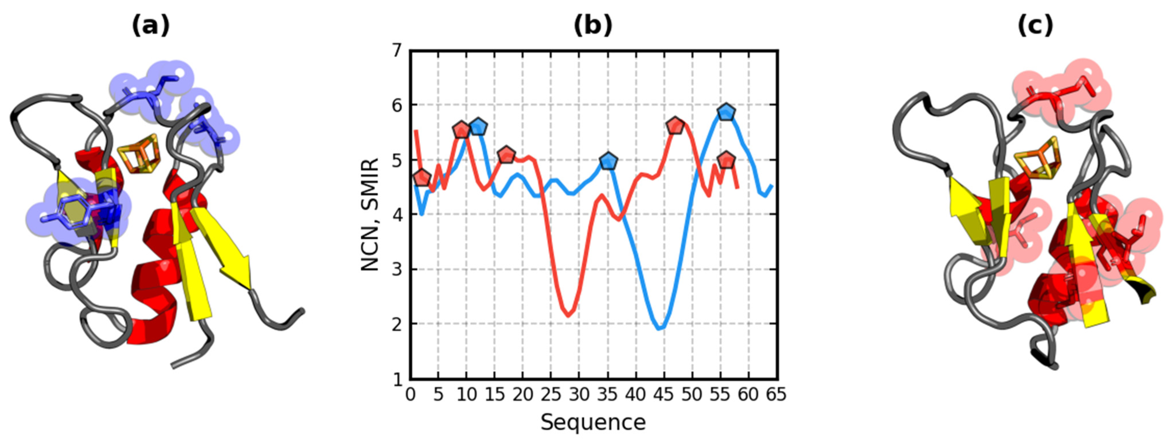
The status of monomer units of FdI and FdII treated as parts of dimers is described by RD values of 0.56 and 0.58, respectively (

Table 3. Hydrophobicity status of monomers of FdI (1FXR) and FdII (1FXD) seen as parts of dimers (3D Gauss capsule fit to the dimer) and their selected fragments. See description of Table 3 for more information how to interpret this table.

Fragment	Residues		RD		TvH		OvT		OvH
	FdI	FdII	FdI	FdII	FdI	FdII	FdI	FdII	FdI	FdII
monomer	chain A	chain A	0.56	0.58	0.16	0.25	0.53	0.31	0.75	0.87
strand A.1	3–6	1–4	0.43	0.32	0.72	0.56	0.46	0.75	0.86	0.96
strand A.2	59–62	55–58	0.25	0.19	0.91	0.92	0.91	1.00	0.76	0.93
sheet A	strand A.1 + A.2	strand A.1 + A.2	0.37	0.38	0.70	0.35	0.57	0.58	0.77	0.87
strand B.1	25–27	22–24	0.19	0.52	0.18	−0.52	0.95	0.00	0.49	0.85
strand B.2	34–36	31–33	0.97	0.19	0.97	0.99	−0.73	0.89	−0.88	0.94
sheet B	strand B.1 + B.2	strand B.1 + B.2	0.35	0.50	0.42	0.11	0.80	0.35	0.45	0.87
all sheets	sheet A + B	sheet A + B	0.33	0.38	0.55	0.31	0.71	0.64	0.71	0.83
no sheets	!(sheet A + B)	!(sheet A + B)	0.59	0.57	0.10	0.14	0.50	0.20	0.76	0.88
helix 1	15–21	13–17	0.27	0.26	0.59	0.74	0.80	0.83	0.88	0.95
helix 2	43–54	41–49	0.64	0.19	−0.09	0.81	0.01	0.86	0.92	0.92
all helices	helix 1 + 2	helix 1 + 2	0.54	0.19	0.20	0.78	0.35	0.86	0.90	0.94
no helices	!(helix 1 + 2)	!(helix 1 + 2)	0.57	0.55	0.16	0.24	0.59	0.39	0.69	0.85
P-P	FdI(P-P)	FdII(P-P)	0.29	0.28	0.90	0.50	0.95	0.82	0.97	0.89
no P-P	!(FdI(P-P))	!(FdI(P-P))	0.54	0.57	0.27	0.30	0.51	0.34	0.78	0.86
P-L	FdI(P-L)	FdII(P-L)	0.77	0.65	−0.28	−0.03	0.06	0.30	0.81	0.69
no P-L	!(FdI(P-L))	!(FdII(P-L))	0.41	0.57	0.35	0.34	0.73	0.36	0.68	0.88
catalytic	11,14,17,54	8,14,50	0.76	0.68	n/a	n/a	0.84	0.38	n/a	n/a
no catalytic	!(11,14,17,54)	!(8,14,50)	0.52	0.58	0.23	0.27	0.60	0.35	0.72	0.86
S-S bond	n/a	18–42	n/a	0.51	n/a	0.33	n/a	0.42	n/a	0.91
no S-S bond	n/a	!(18–42)	n/a	0.53	n/a	0.35	n/a	0.34	n/a	0.83

).

Note that “parts of dimers” above means that T and O distributions were calculated for each dimer as a whole (3D Gauss capsule fit to its two monomers together), after which segments of T, O and H matching the range of chain A (~50% of dimer drop’s data) were extracted and normalized, yielding the status of “monomer as part of dimer”.

RD above 0.5 means that the individual chains do not fit, as a whole, into expected hydrophobicity distribution when the 3D Gauss capsule encompasses them both. Values for the complete complex (both chains together) are similar: 0.55 for FdI and 0.58 for FdII. One explanation has already been given in the previous section: when monomers with a globular shape bind using mostly polar residues, center of the drop ellipsoid (where high concentration of hydrophobicity is expected) is taken by a double amount of mostly polar residues. The second reason can be seen in Table 3 and Figure 5: local discordance between T and O happens in many locations.

Beta fragment 31–33 becomes very accordant in dimeric form of FdII. Being hydrophobic and close to the center of the complex allows its T value to raise and reach RD of 0.19. Because its corresponding fragment in FdI (34–36) is located on the outside of the dimer, it remains discordant with an almost-maximal RD value of 0.97.

The RD status of P-P interface increases from 0.18 to 0.28 in FdII but drops to 0.29 from 0.46 in FdI. This is an effect of tightly packed residues in the center of FdI complex, which allows them to gather more hydrophobicity from the neighbor chain and provide with O what T is expecting at that location. This accordance is mostly caused by G23, G41 and A42, which seem to “work” towards the local and global complex accordance. On the other hand, accordance in FdII interface seems to be held by V32, the residue with highest observed hydrophobicity closest to the center of the drop (but also to the ligand—before it in the sequence is a P-L interacting A31).

The RD statuses of residues engaged in ligand binding appear to be much higher than 0.5 in both FdI and FdII complex. This is the consequence of a conformation where binding pockets are oriented away from the center. Their theoretical hydrophobicity must decrease, while their O is unchanged and high due to present cysteines. Because of more elongated dimer structure, this phenomenon is stronger in FdI (RD 0.77 vs. 0.65).

Figure 5 shows how differently complex formations of FdI and FdII affects the T and O distributions in monomers seen as part of FOD drop fit to the dimers. O can be influenced only by the interactions between the chains, which is why it does not change much when compared with data from Figure 4. T however may change drastically, and in this case it, actually, is the reason behind the many RD values above 0.5 in Table 3.

Different dimer conformation between FdI and FdII is signaled by a low (0.41) T vs. T correlation coefficient (Figure S5). Such change may be offset in another molecule (to reach or maintain RD below 0.5) by a considerably large, tightly packed and (preferably) hydrophobic interaction area, with domain swapping and formation of quasi-domains [58] being some of the ways to achieve this outcome. In-complex CC for O vs. O is 0.74.

3.5. SMIR Analysis

Figure 6b presents the distribution of the density of hydrophobicity resulting from the MIR simulation. It appears that a rather high value of this density, at the exception of a well in each of the ferredoxins, is not located at the same position. This minimum—in other words, this high density of hydrophilic residues—occurs around Q44 of FdI, which is included in the major contribution to P-P interface (40–46). A minimum of same value occurs around position G28 of FdII, which is also very close to P-P interface (23–26). This confirms the previous conclusions that the major contribution to P-P is mainly non hydrophobic, with a residual hydrophobic contribution.

Two peaks, defined as SMIR (see Section 2.3) are present in each ferredoxin. Located around C11 and V56 in FdI, and around M9 and D48 in FdII. They correspond to P-L interaction sites—at the exception of the last one (D48 of FdII) displaced by two positions relative to the native P-L site. This may be due to the effect of the smoothing procedure used to derive the SMIR from the number of non-covalent neighbors. These arguments are coherent with the FOD results—a major contribution of hydrophilic patterns to the protein–protein interface—and thus reinforce this assumption.

3.6. Hydrophobicity-Based Ligand Binding Site and Protein–Protein Interface Determination

Determination of ligand binding sites and protein–protein interfaces based on the hydrophobicity distribution provided by FOD model is possible using two methods.

In the first method, the substrates (two or more individual structures: monomers, domains, complexes, etc.) are submitted to a global optimization procedure that aims to minimize the RD of the whole system by starting from some—possibly randomly-selected—conformation. Substrates can move in the space, subject to typical constraints, such as the requirement of having at least one non-bonded contact between them. Such a black box approach (requiring only the tertiary structure) is based on the assumption that hydrophobicity has dominant role in formation of the complex. For example—as mentioned in Section 3.1—chains with hydrophobic patches of significant size or composition present on the surface may “want” to assume a position in the quaternary structure where those patches would face other chains, shielding them from water.

The second prediction method relies on an intermediate step (after T and O profile calculation) where the substrate structures are analyzed and promising candidates for the P-L or P-P interaction sites are selected among the residues. Other non-hydrophobic criteria may also be used here (or perhaps FOD is implemented as a scoring function in another program). Once such putative interface has been selected, a local optimization procedure may begin to construct the complex using it as its starting position.

In this section we focus on the second approach, presenting how to use FOD to search for and present residues that may be involved in non-bonded interactions.

Discrepancies and outliers in the hydrophobicity profile of a protein (O) appearing when compared to the reference distribution (T) can be viewed from global and local perspective, which both provide insight into the characteristic of the molecule. This allows FOD model to act both as a feature exploration and a prediction tool. D_KL (and by extension its derivative—the RD) by itself (without optimization) belongs to the first category. It primarily measures the global accordance/discordance of T vs. O and—if one desires such information—the influence of specific multi-residue parts of the chain (i.e., a helix or a strand) on the structure of the hydrophobic core. In other words, it revolves around the notion of a “distribution” (a data series). This type of analysis concerns the previous sections of Results regarding the ferredoxins.

On the other hand, the local perspective focuses on individual residues with much lower regard for their position within the sequence or assigned secondary structure. Again, this involves observation of the differences between T and O, but this time in a more direct fashion, yet still from the viewpoint of the whole molecule. Due to how these distributions are calculated—like with entropy—there is no universal cut-off at which one could say that, for example, “the difference between T and O for this residue is high/low” (single point accordance or discordance determination) or that “values of T and O are both high/low for this residue” (single point core or surface determination). However, one can instead plot a 2D hydrophobicity map (T vs. O) for a given protein, partition it into segments with size and location depending on the distribution of the residues (specific to this structure) and assign the partitioned residues to feature levels, such as hydrophobic core or a possible protein–protein interaction area.

It should be noted that this classification of individual residues is not entirely new. Its first form has been proposed in [44] and modified versions were used throughout some of the other papers [32,59,60]. However, here we provide not only a formal definition with description of the calculation algorithm but also introduce some important improvements to use now on, hence its appearance in Results rather than in Methods.

A single residue can be assigned to one of five FOD hydrophobicity classes:

• Class C (core)—hydrophobic core: both T and O are relatively high (T↑↑O) and the difference between them is relatively low (|T-O|→0);
• Class S (surf)—hydrophilic surface: both T and O are relatively low (T↓↓O) and the difference between them is relatively low (|T-O|→0);
• Class B (bind)—deficiency of hydrophobicity closer to the center of the molecule, hinting a possible ligand binding pocket: T is relatively high, O is relatively low (T↑↓O) and the difference between them is relatively high (|T-O|→1);
• Class D (dock)—excess of hydrophobicity closer to the outside of the molecule, hinting a possible protein docking interface: T is relatively low, O is relatively high (T↓↑O) and the difference between them is relatively high (|T-O|→1);
• Class Z (zero)—neither of the above: low difference between T and O (T ≈ O) but also unremarkable position on the T vs. O map (near the average, somewhere in between core and surface)—a model-accordant but hydrophobically insignificant residue.

In addition to the class itself, a residue is also given a hydrophobicity class level which denotes strength of its class membership, directly translating into its significance:

• Level 3 (classes C₃, S₃, B₃ and D₃)—most prominent class members, with strongest defining features, i.e., lowest |T-O| for C and S and highest |T-O| for B and D;
• Level 2 (classes C₂, S₂, B₂ and D₂)—significant class members but not as outstanding on the map as level 3, i.e., low |T-O| for C and S and high |T-O| for B and D;
• Level 1 (classes C₁, S₁, B₁ and D₁)—weak class members, extracted from class Z.

Residues at levels 2 and 3 are the primary class members and may be treated collectively as one level in small proteins, especially in case of core and surface. In larger proteins it might be advisable to start the analysis at level 3. Class Z has no levels.

Class C₂ primarily exists to reduce the chance for incorrect manual classification of residues with very high O or very high T (i.e., a disulfide bond on O profile or a peak on T profile, often due to the chain going through the center of the drop) where the visual difference between the distributions could provoke the researcher to assign a D or B class, contrary to what the statistic is suggesting. This somewhat paradoxically puts most of class C₂ area further away on the map from class Z square than class C₃. Similar situation happens in class S, although there is much lower risk for incorrect assignment by hand here. Automatic classification eliminates any of such problems.

Figure 7 presents a six-step residue classification algorithm of FOD, using FdI as an example. This algorithm differs from previously published papers mostly in the definition of level 1 and level 3 assignment, which makes it more flexible.

Following steps should be performed in order to classify residues from a given protein structure based on their T vs. O hydrophobicity density map:

• (Figure 7a) plot residues as points in T vs. O space (T on the X-axis, O on the Y-axis); calculate quartiles of the T distribution: Q₂ (median), Q₁ (median of T < Q₂) and Q₃ (median of T > Q₂); assign three thresholds: T₁ = Q₁, T₃ = Q₃, T₂ = (Q₁ + Q₃)/2;
• (Figure 7b) draw a T = O line and shift it to point [T₁,T₃]; draw it again and shift it to point [T₃,T₁]; draw a T = -O line and shift it to point [T₁,T₁]; draw it again and shift it to point [T₃,T₃]; four points where pairs of these lines intersect are the class Z square vertexes: v_cd, v_ds, v_sb and v_bc (meaning of indexes is explained in point 5);
• (Figure 7c) extend lines away from class Z square vertexes, partitioning the T vs. O space into five segments, with class Z square in the middle of the map;
• (Figure 7d) place four helper circles symmetrically around class Z square to cut away portions from it to be used as delimiters for level 1 class zones; each circle has T₃-T₁ radius and intersects two nearby class Z square vertexes (i.e., v_cd and v_ds);
• (Figure 7e) remove helper circles except for their arcs within class Z square; give space segments around it following labels: C (core, top-right), D (dock, top-left), S (surf, bottom-left) and B (bind, bottom-right); indexes at names of class Z square vertexes inform between which classes they are located, i.e., v_cd is between C and D;
• (Figure 7f) draw separation lines (v_ds to v_cd and v_sb to v_bc) to demarcate levels within each class; in case of C and S, level 3 is closer (via orthogonal projection) to T = O line than 50% of length of edge of class Z square (i.e., half of the distance between v_cd and v_bc, shown as dashed lines) and level 2 is outside this range; in case of B and D, level 2 is also outside this range, while level 3 is even further away from T = O line: more than 75% of length of edge of class Z square (shown as dotted lines).

T₁, T₂ and T₃ thresholds from step 1 are calculated only for T distribution but are also used for segmentation of the O dimension. This is due to the fact FOD model is testing how well O is reproducing T, which is the principle behind the usage of RD.

Once all residues on the map have been classified, it becomes possible to point to individuals belonging to hydrophobic core, hydrophilic surface surrounding it and any interesting locations within the molecule where discrepancies occur, and which may hint putative interaction areas. As stated previously, FOD model expects those areas to contain residues exhibiting high difference between T and O. That means classes D and B, with D being the “default” class for P-P and B for P-L (hence their names).

3.7. Ligand Binding Site and Protein–Protein Interface Determination in Ferredoxin I and II

Using algorithm from the previous section, we assigned all residues from FdI and FdII monomers to FOD classes in order to check which of them could hint at the native P-P and P-L interaction sites despite low RD. They are visually presented in Figure 8.

Because both proteins are strongly accordant with the model (RD around 0.3), as expected, the number of members of classes D₂ and B₂ is relatively small, with no class D₃ or B₃ representatives and a high number of residues in classes C₃ and S₃—those which are located in their anticipated regions (center and surface of the molecule). They are additionally supported by class Z which also positively contributes to the RD-measured accordance through a “hydrophobic inertia” (by being hydrophobically insignificant but otherwise not counteractive towards the situation in the rest of the molecule).

In FdI there are three residues in class D₂: G23, G41 and V56 and three in class D₁: I12, C14 and A42 (Figure 8a,c). This is not surprising. G23 and G41 were already mentioned previously in the context of being hydrophobic and playing role in stabilization of the complex. They are members of native P-P interface, among five other interacting residues that are scattered mostly (except one) within class Z square. V56—which is a SMIR—is in contact with the ligand and three other residues from the binding site are in its vicinity in the sequence. I12 and C14 also belong to the binding pocket. A42 on the other hand is in the center of the P-P interface. No residues fall into class B₂ zone here, but there are five members of class B₁: F4, Q8, E46 (a P-P contact), E48 and E49, with the last three located in the second helix. It can be seen on Figure 8c that residues engaged in P-L and P-P interaction in FdI gravitate towards the upper fragment of the map.

In FdII the situation is flipped: there is only K30 in class B₂ accompanied by E3 and E12 in class B₁ (Figure 8b,d), engaged in P-P and P-L interaction, respectively. The only representatives of D classes are M9 and A52 at level 1. They surround the ligand. Here contacts are mostly located below the T = O line and, with the exception of K30, they stay in the accordance zone (Figure 8d). K30 is not in any native contact, but A31 (P-L) and V32 (P-P)—which is linked to stability of the complex—are close to it. The C18-C42 disulfide bond is also unsurprisingly high on the map (class C₂).

With all residues classified by FOD, we performed an in silico experiment to check if they are also spatially close to a larger number of native P-P and P-L contacts. If so, this would mean that FOD algorithm may act as a ligand binding or quaternary structure predictor by itself or when joined by other scoring functions. Because there is only a couple of residues present in the important classes, we checked both D₂ and B₂ (each class type separately) but also their D₂ + D₁ and B₂ + B₁ unions (residues at level 2 and 1 together, each class type union also, separately).

Numerical output of this experiment is given for FdI in

Table 4. Comparison of residues engaged in native P-P and P-L interactions in FdI (1FXR) with results of their prediction. There are two clusters constructed from members of class D₂, two from D₂ + D₁ class union and one from B₂ + B₁ class union.

Class	Cluster	NativeP-PContacts	NativeP-LContacts
		23, 38, 40, 41, 42, 43, 46	6, 11, 12, 13, 14, 15, 17, 54, 56, 58, 59
D2	10, 54, 55, 56, 57, 58	∅	(11), 54, 56, 58, (59)
	21, 22, 23, 24, 25, 37, 38, 39, 40, 41, 42	23, 38, 40, 41, 42, (43)	∅
D2 + D1	10, 11, 12, 13, 14, 15, 16, 54, 55, 56, 57, 58	∅	11, 12, 13, 14, 15, (17), 54, 56, 58, (59)
	21, 22, 23, 24, 25, 37, 38, 39, 40, 41, 42, 43, 46	23, 38, 40, 41, 42, 43, 46	∅
B2 + B1	2, 3, 4, 5, 6, 7, 8, 9, 10, 11, 20, 21, 33, 35, 36, 39, 42, 43, 44, 45, 46, 48, 49, 50, 51, 52, 53, 60, 61	(38), (40), (41), 42, 43, 46	6, 11, (12), (54), (59)

Note: cells in Native columns present residue numbers from the native P-P and P-L contacts that are matched by residues from Cluster column in the same row (clustered nearest neighbors of given FOD class members)—the true positive results. Parenthesis denotes gratuitous prediction (1 aa difference in the sequence). Numbers given in bold distinguish actual FOD class members present on the T vs. O map (before clustering). Underline marks D₁/B₁ class members and their nearest neighbors inside the combined D₂ + D₁/B₂ + B₁ clusters (i.e., residues appearing in the results due to union with level 1).

and in

Table 5. Comparison of residues engaged in native P-P and P-L interaction in FdII (1FXD) with results of their prediction. There is one cluster constructed from members of each class/class union (D₂ + D₁, B₂ and B₂ + B₁). See description of Table 4 for information how to interpret this table.

Class	Cluster	NativeP-PContacts	NativeP-LContacts
		3, 23, 24, 25, 26, 32, 37	8, 9, 10, 11, 12, 13, 14, 31, 55, 50
D2 + D1	7, 8, 9, 10, 11, 50, 51, 52, 53, 54	∅	8, 9, 10, 11, (12), 50, (55)
B2	4, 5, 6, 8, 24, 25, 28, 29, 30, 31, 32	(3), (23), 24, 25, (26), 32	8, (9), 31
B2 + B1	1, 2, 3, 4, 5, 6, 8, 10, 11, 12, 13, 14, 15, 16, 24, 25, 28, 29, 30, 31, 32, 54, 55, 56, 58	3, (23), 24, 25, (26), 32	8, (9), 10, 11, 12, 13, 14, 31, 55

for FdII, while visualization for both molecules is presented in Figure 9, although limited to results for level 2 classes for clarity.

A local docking algorithm would primarily search for the optimal conformation around its starting position. To simulate this, we gathered all residues within 3.9 Å from given D and B class members and performed a single-linkage agglomerative clustering on the resulting atoms with a cut-off distance of also 3.9 Å. In addition, we employed a constraint where any two atoms from the same residue were always placed in the same cluster regardless of their distance, although it made no difference here with cut-off of this length. This allowed us however to split the FOD class neighborhood into separate clusters—the individual putative complex interface and ligand cavity search areas. Finally, we left in the output only those residues which were confirmed to be located at most 3.9 Å away from vertexes of the solvent-accessible surface of the proteins to simulate a sensible behavior of a docking algorithm which would not enforce contacts from atoms that are buried away from the surface (again, this had no consequence here).

In FdI (Table 4), G23, G41 and V56 from class D₂ yield two clusters of residues of sizes 6 (around V56) and 11 (around G23 and G41). More numerous of these clusters is located within the native P-P interface, encompassing 5 out of 7 of its members (6 if 1 residue distance in the sequence is permitted). Smaller one is closer to the ligand binding pocket, intersecting 3 (5 at 1-aa distance) out of 11 native P-L contacts. Class B₂ is empty in FdI. Addition of neighbors of residues from class D₁ (I12 and C14) increases size of the V56 cluster by 5 to 11, capturing all native P-P contacts. Number of true positive P-L results around G23 and G41 increases to 8 (10) owing to A42 and its two neighbors. F4, Q8, E46, E48 and E49 from class B₁ gather one large cluster, 29 residues in size. It intersects the native contact set to only a small extent: 3 (6) for P-P and 2 (5) for P-L, but at the same time produces a significantly large number of false positives.

FdII displays lower result variety than FdI (Table 5). It has only a couple of class D₁ members (M9 and A52), with one 10-residue cluster in their neighborhood that has 5 (7 at 1-aa distance) elements in common with native P-L interface out of 10 possible. Furthermore, 11 residues constitute the single cluster around K30, the class B₂ representative. This cluster yields 3 (6) out of 7 true positive P-P contacts and 2 (3) true positive P-L contacts. V32 located close to K30 is also its member. When E3 and E12 from class B₁ bring their neighborhood along the class B₂ results, size of the resulting cluster grows to 25 residues. This switches E3 from gratuitous true positive to direct P-P hit and provides 8 (9) native P-L matches, but again with the cost of higher count of false positive output.

3.8. Comparative Analysis—Type III Antifreeze Protein and Rad50 Domain of Mre11

The two ferredoxins presented in this paper exhibit RD status of their monomers similar to type III antifreeze proteins (or even lower in case of FdII), which are among the best in terms of 3D Gauss function accordance [12]. At the same time biological function of these ferredoxins demands binding of a ligand and formation of a dimer. A type III AFP does neither of this kind of interactions to carry out its own role. This contradiction has led us to the previous section where we have shown that even at a very low (around 0.3 or less) RD level measured at the global scale, which strongly hints a well-ordered hydrophobic core surrounded by polar residues, hydrophobicity density maps of FdI and FdII show finely detailed discrepancies that can be linked back to areas natively associated with P-L and P-P interaction.

Given the above statement, one may ask whether type III AFPs also have similar T vs. O map features. To answer it, we analyzed a representative of this family accessible by PDB code 9MSI. It is naturally a monomer, mostly unstructured, with its size and shape (Figure 1c) slightly resembling FdII (cealign RMSD: 6.61 Å/40 aa, 9.11 Å/48 aa for FdI). RD for the whole molecule is 0.29. All its segments also exhibit very strong accordance (Table S1). A striking similarity can be seen between its T and O profiles (Figure 10a), especially on the map (Figure 10c) where not a single residue falls outside the accordance stripe (marked by the dashed lines). There are no members of D₂, D₃, B₂ and B₃ classes and just three insignificant representatives of class B₁, located deeply within the class Z square: S24, P33 and D36. The accordance classes (C and S) capture most of the residues at third level with only 2 and 8 of them respectively being at level 1. This shows that even with similar RD value, hydrophobicity map characteristic of type III AFP is clearly different from the one exhibited by ferredoxins. It correctly signals that a lack of protein–protein and protein–ligand activity should be expected from it.

The three proteins investigated so far: FdI, FdII and type III AFP are globular, relatively small and highly accordant with 3D Gauss function (RD ≈ 0.3). To showcase how the presented approach handles a vastly different structure, we also included 1L8D in this analysis. It is the PDB code for Rad50 domain from Mre11-Rad50-Nbs1 complex. Its hairpin shape and exposition of all residues to the solvent nearly guarantees that no stable hydrophobic core will be found in it (Figure 1d). The same can be said for its dimer. Monomers interact only by their hook regions surrounding the Zn²⁺/Hg²⁺ ion, with long helices facing away from each other. This results in a large 3D Gauss capsule with a compact, 14-residue P-P contact area (D429, T432, A433, E436, K439, C444, P445, V446, C447, R449, E450, L451, L459 and Y463) that does not allow most of the complex substrates to share a lot of hydrophobicity. Global RD values corroborate these assumptions: 0.70 for monomer, 0.67 for dimer and 0.68 for monomer as part of dimer.

With the exception of two very short 2-aa beta strands, all segments of Rad50 are also discordant (Table S2). This results in hydrophobicity profile shown in Figure 10b. Distribution differences are clearly visible here, with O in the hook region prominently towering over very low T. Its two highest peaks are C444 and C447 which coordinate the zinc/mercury ion. They are class D₃ members, surrounded by their D₂ neighbors: V446, G448 and L451, among which only G448 is not engaged in P-P interaction (Figure 10d). L399, L402, I491 and I495 located at the termini belong to class D₁ (9 total) and suggest—although not as strongly—a putative interaction area there. They probably would not do that if the helices were longer (as they are in vivo) since that would raise T value there due to increased size of the 3D Gauss capsule. There is only one P-P contact in class S₃: E450. In fact, there are only eight class S₃ members, located close to its level 1 boundary.

The saw-like motif visible on T and O profiles of this protein is caused by the helices spinning their residues in and out of the vicinity of the center of the drop, resulting in constantly changing class (C to B). There are 11 members of class B₁ and 4 of B₂ (E415, R419, E422 and K426). All four belong to the same helix and face the same direction.

The “proper” region of the Rad50 hook is marked by Pfam as its 423–474 segment. RD calculation for it has interesting results (Table S3). It is very discordant when seen as part of monomer (0.75) but becomes less unstable as part of dimer (0.6). The hook itself is close to the accordance threshold (0.53, Figure 11a) and crosses it when the 3D Gauss capsule is fitted to the hook/hook complex (0.49, Figure 11b). A single hook segment in such dimer has almost the same RD value. C447 and G448 (level 3) and V446 (level 2) are the D class members here, similar to complete 1L8D PDB data. B class however has different composition: K431, E436, K438 and K462 on level 2 and E435 and D466 on level 1. These residues are closer to the ion than their counterparts from previous paragraph.

Since Hopfner et al. provide dimeric form of Rad50 [27], it is eligible for verification by our P-P and P-L contact exploration and prediction procedure. Due to overlap in the D class between the 1L8D data and its Pfam subset, we decided to apply this procedure to the first. Moreover, due to existence of residues at level 3 and a relatively large number of those at level 1, we focused only on the two significant classes (2 and 3). Results of this prediction are presented in

Table 6. Comparison of residues engaged in native P-P interaction in Rad50 (1L8D) with results of their prediction. There is one cluster constructed from members of each class/class union (D₃, D₃ + D₂ and B₂). See description of Table 4 for more information how to interpret this table.

Class	Cluster	NativeP-PContacts
		429, 432, 433, 436, 439, 444, 445, 446, 447, 449, 450, 451, 459, 463
D3	443, 444, 445, 446, 447, 448, 449, 451	444, 445, 446, 447, 449, (450), 451
D3 + D2	436, 437, 442, 443, 444, 445, 446, 447, 448, 449, 450, 451, 452, 453, 456	436, 444, 445, 446, 447, 449, 450, 451
B2	411, 412, 413, 414, 415, 416, 417, 418, 419, 420, 421, 422, 423, 424, 425, 426, 427, 428, 429, 430, 466, 470, 477	429

, and Figure 10b,d and Figure 12.

Clustering of nearest neighbors of class B₂ members of Rad50 results in all false positives except D429 on a helix. No ligand pocket should exist between the helices, but if one was looking for higher order complex conformation (see Figure 3 of [27]), joining the proteins side by side with residues exhibiting low O value facing each other could bring this distribution closer to T, possibly reaching RD below 0.5. Because the helices are shown to intertwine [27], we may speculate that such class B₂ clusters could be distributed along the whole length of Rad50 until it meets with the rest of its complex.

Results of the prediction look significantly better in D class (Figure 12). As expected, C444 and C447 carry enough information to unveil the native P-P interface. If they were not cysteines, O of the hook region would be lower (possibly achieving only class D₂), but probably still high enough to correctly point to the interaction area there. It should also be able to withstand some degree of rotation of the monomers around the ion.

4. Discussion

The detailed presentation of the proteins discussed in this paper, Ferredoxins I and II, delivers an example of a very high accordance between expectations (3D Gauss function, T distribution) and observed status—O distribution. So far, the best fit of this kind was seen in titin [14] and type III antifreeze proteins [12]. Such molecules present very good examples for fuzzy oil drop model to describe the folding process as micelle formation, which in some proteins occurs along high T vs. O accordance.

Ferredoxins I and II have biological activity in form of electron transfer mediated by an iron-sulfur cluster ligand. The ligand binding cavity, which is located in the same spot in both proteins, is quite large in respect to the length of the chain (64 and 58 residues). Despite its presence, FdI and FdII monomers exhibit a very well-ordered hydrophobic core—high accordance with 3D Gauss function. The pockets, constructed from hydrophobic cysteines (which also coordinate the ligand and as such have their sidechains turned towards inside of the molecule) are accordant in monomers, but become discordant in the dimers where complex formation positions them towards the lower end of T distribution range. This causes strong local discordances defining the locus for ligand binding. It means the biological activity should appear after finalization of quaternary structure construction process. The role of cysteine—especially the role of S-S bonds in respect to hydrophobic core formation—is discussed in detail in [61] (the S-S bond system seems to generally be in opposition to FOD model expectations).

Ferredoxin I and II seem to fold as an individual unit (monomer) incorporating the ligand as consequence of centric hydrophobic core support. Complex formation causes them to lose the accordance status (RD ≥ 0.5). Given the globular shape of the monomers and only seven residues in the P-P interface, this is an expected phenomenon. Based on FOD model data, both dimers seem to be generated through mostly polar interaction, with support (or guide) by hydrophobic interactions from few specific residues. Such a scenario is in agreement with MIR simulations. In FdI these residues appear to be G23 and G41, which are both P-P interface members and are outstanding on monomer T vs. O maps. FdII has V32, but its role becomes visible in the dimer.

An antifreeze type III protein, although it has a very low RD value comparable to the ferredoxins, exhibits vastly different features on the hydrophobicity map. In fact, it can be said that it has no such features at all when one is looking for residues marking a putative P-P or P-L interaction areas (at the significant levels of D and B classes). This observation is however completely correct when function of this protein is considered and confirms that T vs. O map analysis may be used to differentiate between structures which are similar in terms of overall stability of their hydrophobic core.

Clustering of spatial neighbors of residues from ferredoxin monomers which were assigned to D and B classes of FOD shows that there are two perceived “seeds” of discordance in FdI, located at the opposing ends of the molecule. One of them contains the previously mentioned G41 and G23 (class D₂), while the other has only V56 (also D₂) with significant amount of hydrophobicity exposed on the surface, probably gathered from the nearby ligand binding pocket members. These “seeds”, when expanded to their neighborhood and clustered, allow reconstruction of the nearby P-P and P-L interface.

In FdII, which has more accordant monomers with the 3D Gauss function than FdI, only one discordant cluster is registered, originating from K30 (class B₂). This residue has similar physical location to V56 in respect to the ligand but exhibits opposite status (hydrophobicity deficiency rather than excess). Due to different complex formation, K30 is located in between the binding pocket and the P-P interface, capturing residues from both of these regions during the prediction experiment.

FOD-based classification of discordant (RD ≥ 0.5) and non-globular proteins and use of this information to determine their interaction areas is also possible, as shown on the example of Rad50 domain, where the protein–protein interface is resolved almost perfectly by using D class data. Interestingly, when the region closer to this interface is inspected (Pfam coiled-coil zn hook, residues 423–474), it becomes clear that as one limits the calculation to the vicinity of P-P area, the high peak in the central O fragment starts to be “followed” by raising T distribution, causing residues to leave class D for class C (Figure 11). Similar, but weaker phenomenon can be observed in whole 1L8D dataset. This suggests that hydrophobicity may play a role in initial formation of contact between Rad50 units even though the dimer is not hydrophobically stable. It partially fits FOD expectation where accordant complex is made from discordant monomers. It is worth mentioning here that most structures we worked with so far subscribe to “monomers accordant, dimer accordant” and “monomers discordant, dimer discordant” themes.

Classification of FOD residues proposed in this paper has high flexibility, allowing choosing of class level suitable for given structure. Higher level (i.e., 3) means narrower search but focused on the most outstanding data, while lower level (i.e., 1) can be either ignored or included in further analysis, depending on available number of members of significant classes. Alternatively, residues from class Z can be used as a “support”, for example (if there is a lot of them) instead of the nearest neighbors. One must remember however that class Z members will be mostly located between core and surface. Based on the results, in case of FdI and FdII it is not recommended to perform the search on level 1 as it leads to high count of false positive results.

The presented contact prediction method is not without limitations. One of them is intrinsic to the model itself: current algorithm for the orientation of the molecule (for T distribution calculation) is heavily influenced by effective atom outliers. Sometimes a single outstanding residue (i.e., at the termini) may change the size of the 3D Gauss capsule, returning different results between almost identical chains. Second problem is related to the fact that D and B classes are populated with residues from opposite sides of the T₂ threshold. This makes it harder to detect a P-P interface which spans elongated patches on the surface of the monomers which may not exhibit the same hydrophobic quality (i.e., they belong to class Z). Finally, given how P-P and P-L interaction areas may be pointed to by both D and B classes, there is a question how to discern them. Since our approach is an ab initio method, one way to conduct it would be to employ another ab initio method, for example a cavity detector based on the geometric shape of the molecular surface. There are already tools capable of handling this task using various techniques, convex hull being one among them [62,63].

5. Conclusions

The structures of Ferredoxin I and II analyzed in this paper are an exceptional example of highly spherical micelle-like construction with centric concentration of hydrophobicity with the surface covered by polar residues (very low RD value ≈ 0.3). Presence of ligand binding cavity introduces local discordance of observed vs. expected (theoretical) hydrophobicity distribution in the monomer which is not the case in these proteins despite the cavity being rather large in comparison to the whole chain. The discordance however appears in the functional—dimeric form.

Despite having similar sequences in terms of hydrophobicity and identical ligand binding site locations, FdI and FdII present vastly different dimeric formations. Globular structures with such low differences between theoretical and observed distributions (at the scale of complete monomer and its segments) are not expected by the FOD model to form complexes or bind ligands. However, considering T vs. O hydrophobicity map analysis and residue classification protocol presented in this paper it can be seen that even in such highly accordant proteins there are still individual residues that exhibit discordant status, which in this case is enough to constitute a foothold for the search for the native P-P interface and ligand binding cavity, especially the former. While it appears that D class has higher significance in this process, one should also consider B class when looking for putative protein–protein interactions.

Ferredoxins I and II together with type III antifreeze and coiled coil (Rad50) proteins show that FOD model can be used with promising results in the process of quaternary structure prediction of proteins when their tertiary structure is known by pointing out residues which may be engaged in non-bonded contact between the chains. To answer whether hydrophobicity is the actual driving force in complex formation of these molecules one would need to perform RD optimization procedure. On the other hand, in order to verify if (and when) hydrophobicity map analysis is useful for the same purpose when working with other types of proteins, one would need to analyze more (and more varied) structures. Such research will be the object of the future work.

References

1. Burkhart, B.W.; Febvre, H.P.; Santangelo, T.J. Distinct Physiological Roles of the Three Ferredoxins Encoded in the Hyperthermophilic Archaeon Thermococcus kodakarensis. mBio 2019, 10, e02807-18. [Google Scholar] [CrossRef] [Green Version]
2. Maiocco, S.J.; Arcinas, A.J.; Booker, S.J.; Elliott, S.J. Parsing redox potentials of five ferredoxins found within Thermotoga maritima. Protein Sci. 2018, 28, 257–266. [Google Scholar] [CrossRef] [PubMed]
3. Grinberg, A.V.; Hannemann, F.; Schiffler, B.; Müller, J.; Heinemann, U.; Bernhardt, R. Adrenodoxin: Structure, stability, and electron transfer properties. Proteins Struct. Funct. Bioinform. 2000, 40, 590–612. [Google Scholar] [CrossRef]
4. Hsieh, Y.-C.; Liu, M.-Y.; Le Gall, J.; Chen, C.-J. Anaerobic purification and crystallization to improve the crystal quality: Ferredoxin II from Desulfovibrio gigas. Acta Crystallogr. Sect. D Biol. Crystallogr. 2005, 61, 780–783. [Google Scholar] [CrossRef]
5. Im, S.; Liu, G.; Luchinat, C.; Sykes, A.G.; Bertini, I. The solution structure of parsley [2Fe-2S]ferredoxin. Eur. J. Biochem. 1998, 258, 465–477. [Google Scholar] [CrossRef] [PubMed] [Green Version]
6. Raanan, H.; Pike, D.H.; Moore, E.K.; Falkowski, P.G.; Nanda, V. Modular origins of biological electron transfer chains. Proc. Natl. Acad. Sci. USA 2018, 115, 1280–1285. [Google Scholar] [CrossRef] [Green Version]
7. Marco, P.; Kozuleva, M.; Eilenberg, H.; Mazor, Y.; Gimeson, P.; Kanygin, A.; Redding, K.; Weiner, I.; Yacoby, I. Binding of ferredoxin to algal photosystem I involves a single binding site and is composed of two thermodynamically distinct events. Biochim. Biophys. Acta (BBA)—Bioenerg. 2018, 1859, 234–243. [Google Scholar] [CrossRef] [PubMed]
8. Beilke, D.; Weiss, R.; Löhr, F.; Pristovšek, P.; Hannemann, F.; Bernhardt, R.; Rüterjans, H. A New Electron Transport Mechanism in Mitochondrial Steroid Hydroxylase Systems Based on Structural Changes upon the Reduction of Adrenodoxin†. Biochemistry 2002, 41, 7969–7978. [Google Scholar] [CrossRef]
9. Goodfellow, B.; Macedo, A.L.; Rodrigues, P.; Moura, I.; Wray, V.; Moura, J.J.G. The solution structure of a [3Fe-4S] ferredoxin: Oxidised ferredoxin II from Desulfovibrio gigas. JBIC J. Biol. Inorg. Chem. 1999, 4, 421–430. [Google Scholar] [CrossRef]
10. Konieczny, L.; Roterman, I. Globular or ribbon-like micelle. In From Globular Proteins to Amyloids; Elsevier: Amsterdam, The Netherlands, 2020; pp. 41–54. [Google Scholar] [CrossRef]
11. Gadzała, M.; Dułak, D.; Kalinowska, B.; Baster, Z.; Bryliński, M.; Konieczny, L.; Banach, M.; Roterman, I. The aqueous environment as an active participant in the protein folding process. J. Mol. Graph. Model. 2019, 87, 227–239. [Google Scholar] [CrossRef]
12. Banach, M.; Konieczny, L.; Roterman, I. Why do antifreeze proteins require a solenoid? Biochimie 2018, 144, 74–84. [Google Scholar] [CrossRef] [PubMed]
13. Kalinowska, B.; Banach, M.; Wiśniowski, Z.; Konieczny, L.; Roterman, I. Is the hydrophobic core a universal structural element in proteins? J. Mol. Model. 2017, 23, 205. [Google Scholar] [CrossRef] [PubMed] [Green Version]
14. Banach, M.; Konieczny, L.; Roterman, I. The fuzzy oil drop model, based on hydrophobicity density distribution, generalizes the influence of water environment on protein structure and function. J. Theor. Biol. 2014, 359, 6–17. [Google Scholar] [CrossRef] [PubMed] [Green Version]
15. Roterman, I.; Banach, M.; Konieczny, L. Application of the Fuzzy Oil Drop Model Describes Amyloid as a Ribbonlike Micelle. Entropy 2017, 19, 167. [Google Scholar] [CrossRef] [Green Version]
16. Banach, M.; Konieczny, L.; Roterman, I. The Amyloid as a Ribbon-Like Micelle in Contrast to Spherical Micelles Represented by Globular Proteins. Molecules 2019, 24, 4395. [Google Scholar] [CrossRef] [Green Version]
17. Andrusier, N.; Mashiach, E.; Nussinov, R.; Wolfson, H.J. Principles of flexible protein-protein docking. Proteins Struct. Funct. Bioinform. 2008, 73, 271–289. [Google Scholar] [CrossRef] [Green Version]
18. Janin, J. Welcome to CAPRI: A Critical Assessment of PRedicted Interactions. Proteins Struct. Funct. Bioinform. 2002, 47, 257. [Google Scholar] [CrossRef]
19. Available online: https://www.ebi.ac.uk/pdbe/complex-pred/capri (accessed on 23 June 2021).
20. Berman, H.; Westbrook, J.; Feng, Z.; Gilliland, G.; Bhat, T.N.; Weissig, H.; Shindyalov, I.N.; Bourne, P.E. The Protein Data Bank. Nucleic Acids Res. 2000, 28, 235–242. [Google Scholar] [CrossRef] [Green Version]
21. Available online: https://www.rcsb.org (accessed on 18 October 2020).
22. Sillitoe, I.; Dawson, N.; Lewis, T.E.; Das, S.; Lees, J.G.; Ashford, P.; Tolulope, A.; Scholes, H.; Senatorov, I.; Bujan, A.; et al. CATH: Expanding the horizons of structure-based functional annotations for genome sequences. Nucleic Acids Res. 2019, 47, D280–D284. [Google Scholar] [CrossRef] [Green Version]
23. Available online: https://www.cathdb.info (accessed on 22 October 2020).
24. Sery, A.; Housset, D.; Serre, L.; Bonicel, J.; Hatchikian, C.; Frey, M.; Roth, M. Crystal Structure of the Ferredoxin I from Desulfovibrio africanus at 2.3-.ANG. Resolution. Biochemistry 1994, 33, 15408–15417. [Google Scholar] [CrossRef]
25. Kissinger, C.R.; Sieker, L.C.; Adman, E.T.; Jensen, L.H. Refined crystal structure of ferredoxin II from Desulfovibrio gigas at 1.7 Å. J. Mol. Biol. 1991, 219, 693–715. [Google Scholar] [CrossRef]
26. Graether, S.P.; DeLuca, C.I.; Baardsnes, J.; Hill, G.A.; Davies, P.L.; Jia, Z. Quantitative and Qualitative Analysis of Type III Antifreeze Protein Structure and Function. J. Biol. Chem. 1999, 274, 11842–11847. [Google Scholar] [CrossRef] [PubMed] [Green Version]
27. Hopfner, K.-P.; Craig, L.; Moncalian, G.; Zinkel, R.A.; Usui, T.; Owen, B.A.L.; Karcher, A.; Henderson, B.; Bodmer, J.-L.; McMurray, C.T.; et al. The Rad50 zinc-hook is a structure joining Mre11 complexes in DNA recombination and repair. Nature 2002, 418, 562–566. [Google Scholar] [CrossRef] [PubMed]
28. Laskowski, R.A.; Jabłońska, J.; Pravda, L.; Vařeková, R.S.; Thornton, J.M. PDBsum: Structural summaries of PDB entries. Protein Sci. 2018, 27, 129–134. [Google Scholar] [CrossRef]
29. Available online: https://www.ebi.ac.uk/pdbsum (accessed on 19 March 2021).
30. Mistry, J.; Chuguransky, S.; Williams, L.; Qureshi, M.; Salazar, G.A.; Sonnhammer, E.L.L.; Tosatto, S.C.E.; Paladin, L.; Raj, S.; Richardson, L.J.; et al. Pfam: The protein families database in 2021. Nucleic Acids Res. 2020, 49, D412–D419. [Google Scholar] [CrossRef]
31. Kalinowska, B.; Banach, M.; Konieczny, L.; Roterman, I. Application of Divergence Entropy to Characterize the Structure of the Hydrophobic Core in DNA Interacting Proteins. Entropy 2015, 17, 1477–1507. [Google Scholar] [CrossRef] [Green Version]
32. Banach, M.; Fabian, P.; Stapor, K.; Konieczny, L.; Roterman, A.I. Structure of the Hydrophobic Core Determines the 3D Protein Structure—Verification by Single Mutation Proteins. Biomolecules 2020, 10, 767. [Google Scholar] [CrossRef]
33. Konieczny, L.; Roterman, I. Description of the fuzzy oil drop model. In From Globular Proteins to Amyloids; Elsevier: Amsterdam, The Netherlands, 2020; pp. 1–11. [Google Scholar] [CrossRef]
34. Levitt, M. A simplified representation of protein conformations for rapid simulation of protein folding. J. Mol. Biol. 1976, 104, 59–107. [Google Scholar] [CrossRef]
35. Banach, M.; Konieczny, L.; Roterman, I. The active site in a single-chain enzyme. In From Globular Proteins to Amyloids; Elsevier: Amsterdam, The Netherlands, 2020; pp. 71–78. [Google Scholar] [CrossRef]
36. Kullback, S.; Leibler, R.A. On Information and Sufficiency. Ann. Math. Stat. 1951, 22, 79–86. [Google Scholar] [CrossRef]
37. Banach, M.; Konieczny, L.; Roterman, I. Composite structures. In From Globular Proteins to Amyloids; Elsevier: Amsterdam, The Netherlands, 2020; pp. 117–133. [Google Scholar] [CrossRef]
38. Fabian, P.; Banach, M.; Stapor, K.; Konieczny, L.; Ptak-Kaczor, M.; Roterman, I. The Structure of Amyloid versus the Structure of Globular Proteins. Int. J. Mol. Sci. 2020, 21, 4683. [Google Scholar] [CrossRef]
39. Dułak, D.; Gadzała, M.; Stapor, K.; Fabian, P.; Konieczny, L.; Roterman, I. Folding with active participation of water. In From Globular Proteins to Amyloids; Elsevier: Amsterdam, The Netherlands, 2020; pp. 13–26. [Google Scholar] [CrossRef]
40. Banach, M.; Konieczny, L.; Roterman, I. Protein-protein interaction encoded as an exposure of hydrophobic residues on the surface. In From Globular Proteins to Amyloids; Elsevier: Amsterdam, The Netherlands, 2020; pp. 79–89. [Google Scholar] [CrossRef]
41. Banach, M.; Konieczny, L.; Roterman, I. Ligand binding cavity encoded as a local hydrophobicity deficiency. In From Globular Proteins to Amyloids; Elsevier: Amsterdam, The Netherlands, 2020; pp. 91–93. [Google Scholar] [CrossRef]
42. Papandreou, N.; Berezovsky, I.N.; Lopes, A.; Eliopoulos, E.; Chomilier, J. Universal positions in globular proteins: From observation to simulation. Eur. J. Biochem. 2004, 271, 4762–4768. [Google Scholar] [CrossRef]
43. Prudhomme, N.; Chomilier, J. Prediction of the protein folding core: Application to the immunoglobulin fold. Biochimie 2009, 91, 1465–1474. [Google Scholar] [CrossRef] [PubMed]
44. Banach, M.; Prudhomme, N.; Carpentier, M.; Duprat, E.; Papandreou, N.; Kalinowska, B.; Chomilier, J.; Roterman, I. Contribution to the Prediction of the Fold Code: Application to Immunoglobulin and Flavodoxin Cases. PLoS ONE 2015, 10, e0125098. [Google Scholar] [CrossRef] [PubMed]
45. The PyMOL Molecular Graphics System; Version 2.0; Schrödinger, LLC: New York, NY, USA.
46. Available online: https://pymol.org (accessed on 5 October 2020).
47. Hunter, J.D. Matplotlib: A 2D Graphics Environment. Comput. Sci. Eng. 2007, 9, 90–95. [Google Scholar] [CrossRef]
48. Virtanen, P.; Gommers, R.; Oliphant, T.E.; Haberland, M.; Reddy, T.; Cournapeau, D.; Burovski, E.; Peterson, P.; Weckesser, W.; Bright, J.; et al. SciPy 1.0: Fundamental algorithms for scientific computing in Python. Nat. Methods 2020, 17, 261–272. [Google Scholar] [CrossRef] [PubMed] [Green Version]
49. Harris, C.R.; Millman, K.J.; van der Walt, S.J.; Gommers, R.; Virtanen, P.; Cournapeau, D.; Wieser, E.; Taylor, J.; Berg, S.; Smith, N.J.; et al. Array programming with NumPy. Nature 2020, 585, 357–362. [Google Scholar] [CrossRef] [PubMed]
50. Kawabata, T. MATRAS: A program for protein 3D structure comparison. Nucleic Acids Res. 2003, 31, 3367–3369. [Google Scholar] [CrossRef] [Green Version]
51. Available online: http://strcomp.protein.osaka-u.ac.jp/matras (accessed on 28 October 2020).
52. Sanner, M.F.; Olson, A.J.; Spehner, J.-C. Reduced surface: An efficient way to compute molecular surfaces. Biopolymers 1996, 38, 305–320. [Google Scholar] [CrossRef]
53. Available online: http://mgltools.scripps.edu/packages/MSMS (accessed on 25 June 2021).
54. Shanthirabalan, S.; Chomilier, J.; Carpentier, M. Structural effects of point mutations in proteins. Proteins Struct. Funct. Bioinform. 2018, 86, 853–867. [Google Scholar] [CrossRef] [Green Version]
55. Carpentier, M.; Chomilier, J. Protein multiple alignments: Sequence-based versus structure-based programs. Bioinformatics 2019, 35, 3970–3980. [Google Scholar] [CrossRef]
56. Konieczny, L.; Roterman, I. Information encoded in protein structure. In From Globular Proteins to Amyloids; Elsevier: Amsterdam, The Netherlands, 2020; pp. 27–39. [Google Scholar] [CrossRef]
57. Shindyalov, I.N.; Bourne, P.E. Protein structure alignment by incremental combinatorial extension (CE) of the optimal path. Protein Eng. Des. Sel. 1998, 11, 739–747. [Google Scholar] [CrossRef] [PubMed]
58. Dygut, J.; Kalinowska, B.; Banach, M.; Piwowar, M.; Konieczny, L.; Roterman, I. Structural Interface Forms and Their Involvement in Stabilization of Multidomain Proteins or Protein Complexes. Int. J. Mol. Sci. 2016, 17, 1741. [Google Scholar] [CrossRef] [Green Version]
59. Banach, M.; Stapor, K.; Konieczny, L.; Fabian, P.; Roterman, I. Downhill, Ultrafast and Fast Folding Proteins Revised. Int. J. Mol. Sci. 2020, 21, 7632. [Google Scholar] [CrossRef]
60. Roterman, I.; Stapor, K.; Fabian, P.; Konieczny, L.; Banach, M. Model of Environmental Membrane Field for Transmembrane Proteins. Int. J. Mol. Sci. 2021, 22, 3619. [Google Scholar] [CrossRef] [PubMed]
61. Banach, M.; Kalinowska, B.; Konieczny, L.; Roterman, I. Role of Disulfide Bonds in Stabilizing the Conformation of Selected Enzymes—An Approach Based on Divergence Entropy Applied to the Structure of Hydrophobic Core in Proteins. Entropy 2016, 18, 67. [Google Scholar] [CrossRef] [Green Version]
62. Le Guilloux, V.; Schmidtke, P.; Tuffery, P. Fpocket: An open source platform for ligand pocket detection. BMC Bioinform. 2009, 10, 168. [Google Scholar] [CrossRef] [PubMed] [Green Version]
63. Zhao, R.; Cang, Z.; Tong, Y.; Wei, G.-W. Protein pocket detection via convex hull surface evolution and associated Reeb graph. Bioinformatics 2018, 34, i830–i837. [Google Scholar] [CrossRef]
Figure 1. 3D presentation of structures under consideration: FdI (1FXR) (a), FdII (1FXD) (b), type III AFP (9MSI) (c) and Rad50 domain (1L8D) (d). Green segments on (a,b) denote residues engaged in non-bonded interaction with the ligand (atomic distance within 3.9 Å), with its coordinating cysteines shown in lighter color (lime). Purple segments and lines on (a,b,d) mark the location of protein–protein interface (also within 3.9 Å distance). The single disulfide bond in FdII (C18-C42) is shown on (b) as brown sticks. Violet/blue segments on (d) correspond to Pfam coiled-coil zn region in Rad50 (residues 423–474).
Applsci 11 08514 g001
Figure 2. Sequence comparison of FdI (1FXR) and FdII (1FXD) after sequence alignment, split into 1–32 (a) and 33–64 (b) segments. Six insertions in FdII sequence are marked in the central (unlabeled) row with a star, sequence identity with pipe, similar intrinsic hydrophobicity values (H parameter difference ≤ 0.2) with tilde and highly different intrinsic hydrophobicity values (H parameter difference > 0.4) with cross. Horizontal bars denote secondary structure motifs: pink—helix, amber—sheet, purple triangles—P-P interaction, teal triangles—P-L interaction and white diamonds—ligand-coordinating cysteines. H parameter values are expressed by colors of the circles with amino acid codes: closer to blue—more hydrophilic, closer to red—more hydrophobic and closer to green—towards the middle of hydrophobicity scale.
Applsci 11 08514 g002
Figure 3. Comparison of hydrophobicity parameter values of FdI (1FXR) and FdII (1FXD) after sequence alignment, in 1-D (a) and in 2-D (b). H parameter values for FdI is shown on (a) as bars growing upwards from the 0.0 line, while corresponding data bars for FdII grow downwards. Color of each bar pair and of their corresponding marker on (b) symbolizes the absolute H parameter difference between the two proteins for a given pair of residues (i.e., blue—low, yellow—medium and purple—high). Cyan bars present only on top side on (a) locate the six insertions in FdII sequence—they do not appear on (b). H parameter differences higher than 0.4 are treated as outliers. Horizontal bars at the top and bottom of (a) denote secondary structure motifs: pink—helix and amber—sheet. Dashed line on (b) marks line of H parameter identity.
Applsci 11 08514 g003
Figure 4. Hydrophobicity density profiles of monomers of FdI (1FXR) (a) and FdII (1FXD) (b,c). Profile on (b) is the profile from (c) after sequence alignment (six insertions: two at each terminus and two within the chain, marked by distribution discontinuities). Blue lines—theoretical (T) hydrophobicity profile and red lines—observed (O) hydrophobicity profile. Horizontal bars at the top denote secondary structure motifs: pink—helix, amber—sheet. Purple triangles—P-P interaction, teal triangles—P-L interaction and white diamonds—ligand-coordinating cysteines. Brown dashed curve on (b,c) is the C18-C42 disulfide bond.
Applsci 11 08514 g004
Figure 5. Hydrophobicity density profiles of monomers of FdI (1FXR) (a) and FdII (1FXD) (b,c) seen as parts of dimers (3D Gauss capsule fit to the dimer). See description of Figure 4 for more information how to interpret this figure.
Applsci 11 08514 g005
Figure 6. Hydrophobicity density distribution resulting from MIR model simulation (NCN—non-covalent neighbors and smoothed most interacting residues—SMIR) for FdI (1FXR) (a,b) and FdII (1FXD) (b,c). Blue pentagons on (b) and blue spheres on (a) denote SMIRs in FdI (I12, Y35 and V56). Red pentagons on (b) and red spheres on (c) denote SMIRs in FdII (I2, M9, I17, I47 and V56).
Applsci 11 08514 g006
Figure 7. Visualization of algorithm for residue assignment to FOD classes using FdI (1FXR) monomer as an example: (a) calculation of T distribution thresholds, (b) determination of class Z square vertexes, (c) partition of the T vs. O space into five segments, (d) drawing of helper circles, (e) cutting arcs out of helper circles by leaving only their intersection with class Z square and (f) final assignment of residues to classes (C, S, D, B and Z) and to their three levels (1, 2, 3).
Applsci 11 08514 g007
Figure 8. Hydrophobicity density profiles and maps of monomers of FdI (1FXR) (a,c) and FdII (1FXD) (b,d). Residues belonging to core class are shown as red octagons (C2 and C3—large and C1—small), surf class—blue squares (S3—large and S1—small), dock class—purple pluses (D2—large and D1—small) and bind class—teal crosses (B2—large and B1—small). Orange and cyan lines on (a,b) and corresponding orange and cyan circles on (c,d) mark residue clusters located within the protein body in the spatial neighborhood of members of classes D2 and B2. See description of Figure 4 for more information how to interpret this figure.
Applsci 11 08514 g008
Figure 9. 3D presentation of results of FOD-based prediction of P-P and P-L interaction in FdI (1FXR) (a,c,e) and FdII (1FXD) (b,d,e). Native interfaces are shown on (a,b): purple—P-P and green—P-L. Residues belonging to classes D2 and B2 (spheres) and surfaces marking their clustered spatial neighborhood are shown on (c,d). Each cluster is marked using different color. There are two class D2 clusters in FdI (orange and cyan) one class B2 cluster in FdII (orange). Surfaces on (e,f) denote the intersection of data from (c,d) with native contacts from (a,b)—the true positive results.
Applsci 11 08514 g009
Figure 10. Hydrophobicity density profiles and maps of monomers of type III AFP (9MSI) (a,c) and Rad50 (1L8D) (b,d). Orange and cyan lines on (a,b) and corresponding orange and cyan circles on (c,d) mark residue clusters located within the protein body in the spatial neighborhood of members of classes D3, D2 and B2. See description of Figure 8 for more information how to interpret this figure.
Applsci 11 08514 g010
Figure 11. Hydrophobicity density profiles of Pfam coiled-coil zn hook region (residues 423–474) of Rad50 (1L8D) seen in its monomeric (a) and dimeric forms (b). See description of Figure 4 for more information how to interpret this figure.
Applsci 11 08514 g011
Figure 12. 3D presentation of results of FOD-based prediction of P-P interaction in Rad50 (1L8D). Native P-P interface is shown on (a), prediction output (class D3 + D2 cluster—orange, class B2 cluster—cyan) on (b) and its intersection with native data on (c). Violet/blue segments correspond to Pfam coiled-coil zn hook region (residues 423–474). See description of Figure 9 for more information how to interpret this figure.
Applsci 11 08514 g012