Article

Optical Turbulence Profile Forecasting and Verification in the Offshore Atmospheric Boundary Layer

1
Key Laboratory of Atmospheric Optics, Anhui Institute of Optics and Fine Mechanics, Hefei Institutes of Physical Science, Chinese Academy of Sciences, Hefei 230031, China
2
Science Island Branch of Graduate School, University of Science and Technology of China, Hefei 230026, China
3
Advanced Laser Technology Laboratory of Anhui Province, Hefei 230037, China
4
School of Atmospheric Sciences, Sun Yat-sen University, Zhuhai 519000, China
*
Author to whom correspondence should be addressed.
Appl. Sci. 2021, 11(18), 8523; https://doi.org/10.3390/app11188523
Submission received: 26 August 2021 / Revised: 8 September 2021 / Accepted: 9 September 2021 / Published: 14 September 2021
(This article belongs to the Section Earth Sciences)

Abstract

:
A backpropagation neural network (BPNN) approach is proposed for the forecasting and verification of optical turbulence profiles in the offshore atmospheric boundary layer. To better evaluate the performance of the BPNN approach, the Holloman Spring 1999 thermosonde campaigns (HMNSP99) model for outer scale, and the Hufnagel/Andrew/Phillips (HAP) model for a single parameter are selected here to estimate profiles. The results have shown that the agreement between the BPNN approach and the measurement is very close. Additionally, statistical operators are used to quantify the performance of the BPNN approach, and the statistical results also show that the BPNN approach and measured profiles are consistent. Furthermore, we focus our attention on the ability of the BPNN approach to rebuild integrated parameters, and calculations show that the BPNN approach is reliable. Therefore, the BPNN approach is reasonable and remarkable for reconstructing the strength of optical turbulence of the offshore atmospheric boundary layer.

1. Introduction

The atmospheric boundary layer is an important bridge for the exchange of momentum, heat, and water vapor between the earth’s surface and the free atmosphere [1]. The strength of optical turbulence is high in the atmospheric boundary layer, which is a distinctive feature that distinguishes the boundary layer from other atmospheric layers. Atmospheric turbulence is the primary reason for laser beam wandering and spreading, and it leads to a serious degradation of image quality and clarity in optical applications. Atmospheric turbulence strength is generally characterized by the structural constant of the refractive index. The fluctuations of the refractive index of the atmosphere ( C n 2 ) , also known as optical turbulence, are produced by wind blowing over the earth’s surface and temperature gradients between this surface and the air above it [2]. Because of the complexity of atmospheric phenomena, the C n 2 field has a complicated spatio-temporal structure. Problems such as with the intermittent vertical profile make quantitative modeling of optical turbulence a challenging task [3]. Therefore, it is of great significance to accurately estimate the optical turbulence in the atmospheric boundary layer.
Conventionally, C n 2 can be derived using several techniques such as radiosonde, radar, and optical remote sensing, among others [4,5,6,7]. Furthermore, high-frequency wind/temperature measurement instruments are widely utilized, including ultrasonic anemometers and micro-thermometers [8,9]. In 1968, one of the first experiments, the Kansas experiment, was organized outside Liberal, Kansas, USA, to solve the problem in boundary layer research. A sonic anemometer and a platinum wire sensor were installed on a 32 m tower [10]. A second experiment, known as the Minnesota experiment, was performed near Donaldson, Minnesota, USA, in 1973, where a 32 m tower was also installed and a large balloon with turbulence probes was attached to a flying cable. Since the 1970s, many investigations have been performed to determine turbulence height profiles [11]. Coulman analyzed temperature fluctuations in the lowest 200 m of the atmosphere in Culgoora, Australia, in January 1972 with the aid of resistance thermometers and anemometers used at different heights under a captive balloon [12,13]. Bufton, Azouit et al., and McHugh et al. employed two micro-thermal probes placed 1 m apart under a balloon to measure temperature fluctuations up to more than 20 km above the ground [14,15,16,17].
Over the years, several models have been developed that calculate the C n 2 profile. Firstly, the simplest empirical model can be derived from the use of segmented fitting on experimental data, requiring only the input of an altitude variable. For example, the submission laser communication (SLC) model, the Air Force Geophysics Laboratory (AFGL) and Air Force Maui Optical Station (AMOS) model, and the Critical Laser Enhancing Atmospheric Research (CLEAR I) model [18,19,20,21]. Secondly, a parameterization model can be used, based on the basic theory of turbulence to establish the relationship between conventional meteorological parameters and the profiles of C n 2 through the outer scale, such as with the Hufnagel model and Tatarski model [22,23]. Furthermore, another method to forecast the C n 2 profile is given by Felton and Alliss [24], who estimate C n 2 with the use of the weather research and forecast (WRF) numerical weather prediction (NWP) model. However, due to uncertain parameters of this model, the profiles offered by such a model are unsatisfactory. Meanwhile, based on the baroclinic energy of the atmosphere, Kovadlo and Lukin obtained C n 2 profiles of the atmospheric boundary layer using the energy spectrum of the turbulence, ranging from large-scale atmospheric fluctuations to small-scale turbulent fluctuations [25]. Each the conventional method has its own advantages and limitations, and no method is known to be superior [26]. With the development of machine learning theory, neural networks have been gaining interest [27,28,29]. Tracey and Duraisamy employed a neural network to attempt to learn the Spalart–Allmaras turbulence model [30]. This work represents an important step in the use of machine learning algorithms for generalization. Wang and Basu estimated surface-layer optical turbulence at Mauna Loa, Hawaii, and used a Monte Carlo-type approach to optimize the artificial neural network weights and subsequent prediction of C n 2 [31]. Su and Wu et al. developed a new hybrid neural network that combines the backpropagation neural net-work (BPNN) and the adaptive niche-genetic algorithm (AGA) to forecast the near-surface C n 2 [32]. Compared with conventional empirical and parametric model methods, the network method has strong nonlinear mapping capabilities for learning adaptively and is data-driven rather than reliant on empirical formulas.
This research proposes a new method for estimating C n 2 profiles with the use of machine learning. The backpropagation (BP) neural network, called BPNN, is designed to forecast C n 2 profiles in the offshore atmospheric boundary layer, with special consideration of input and output variables. The BPNN is validated against in situ measurements with the spatial evolution characteristic of the C n 2 profiles. Compared with the existing model, we concluded that the BPNN approach is reasonable and remarkable. The remainder of this paper is organized as follows: Section 2 introduces three methodologies associated with the investigation of the C n 2 profiles, Section 3 provides the experimental results and discussion, including the use of contrast experiments, and finally, Section 4 concludes the paper and proposes some limitations.

2. Optical Turbulence Forecasting

2.1. BPNN

The backpropagation neural network (BPNN) was developed by Rumelhart et al. as a solution to the problem of training multi-layer perceptions [33]. It is a feed-forward neural network, and its learning process is shown in Figure 1. First, the original data need to be normalized before the initial weight distributions and thresholds of the network are randomly selected. The input and output parameters, and correction errors of each element in the middle layers, are calculated according to the activation function. Then, the connection weights and thresholds for each layer are adjusted based on acquired errors. After that, learning times are updated to determine whether the errors conform to the allowed range. If so, anti-normalization results are output; otherwise, input, output, and errors are recalculated until the error satisfies the demand. As an artificial intelligence neural network, BPNN has many advantages. First, it is fast, simple, and easy to program. Secondly, it has no parameters to tune apart from the numbers of input. Thirdly, it is a flexible method that does not require prior knowledge about the network, and finally, it does not need any special mention of the features of the function to be learned.
To simplify the model, the input threshold is set to 0. Suppose that given N samples, the output of the k sample at the node i of the l − 1 layer is O u t i k l 1 . Then, the input of the k sample at the node j of the l layer is:
I n j k l = i ω i j l 1 O u t i k l 1
where O u t i k l 1 represents the output of the node i of the l − 1 layer, when the k sample is input. ω i j l i represents the weight coefficient from the node i of the l − 1 layer to the node j of the l layer. After calculating I n j k l , the output of node j of the l layer of the k sample can be calculated:
O u t j k l = f ( I n j k l )
Among them, f is used as an activation function and has many manifestations. This article selects the commonly used sigmoid function in BPNN as the activation function, namely:
f ( x ) = 1 1 + e x
Calculate the error according to the specified expected output, where the commonly used error performance function is square:
E k = 1 2 j ( y j k y ¯ j k ) 2
y ¯ j k is the actual output of node j in the output layer, and y j k represents the expected output. The total error is:
E = 1 2 N k = 1 N E k
Define δ j k l = E k / I n j k l as the partial derivative of the error of the k sample to the j node of the l layer, then the partial derivative of the connection weight is:
E k ω i j l 1 = E k I n j k l I n j k l ω i j l = E k I n j k l O u t i k l 1 = δ j k l O u t i k l 1
Subsequent reverse calculation weight correction. First, calculate the weight correction from the i node in the hidden layer (the l layer) to the j node in the output layer (the l + 1 layer). Then, calculate the weight correction from the h node in the input layer (the l − 1 layer) to the i node in the hidden layer. The result is as follows:
E k ω i j l = O u t i k l 1 ( y k y ¯ k ) f ( I n j k l )
E k ω h i l 1 = O u t h k l 2 j δ j k l ω j i l f ( I n i k l 1 )
where Equation (7) represents the weight correction from the hidden layer to the output layer, and Equation (8) represents the weight correction from the input layer to the hidden layer. Finally, modify the weight, where μ is the step size:
ω i j = ω i j μ E ω i j , μ > 0
E ω i j = k = 1 N E k ω i j
Conventionally, input data divisions are termed as training, validation, and testing data. The training section uses a specific network structure and a fixed number of hidden nodes to learn the characteristics of the data. The verification section is used to prevent the network from overfitting the data, which will inadvertently reduce the generality of its predictions. After the network is fully configured (based on training and verification), the test section will provide an independent evaluation of network performance.

2.2. C n 2 Estimation Model

C n 2 estimation models that convert standard meteorological data into C n 2 vertical profiles are established based on the basic theory of turbulence. According to Kolmogorov’s theory, the Tatarski C n 2 model is [34]:
C n 2 = a L 0 4 / 3 M 2
where a is a constant of 2.8 [35], L 0 is the outer scale, or rather, the largest scale of inertial range turbulence, and M is the potential refractive index gradient defined as:
M = ( 79 × 10 6 P T ) ln θ h
θ = T ( 1000 P ) 0.286
M is related to atmospheric temperature ( T ) , atmospheric pressure ( P ) , and potential temperature ( θ ) . h is the height above ground. From Equations (11)–(13) it can be noted that the vertical temperature gradient can be estimated from sounding data, so choosing the appropriate L 0 is the key to estimating C n 2 . At present, the HMNSP99 model represents the most widely used outer scale model [36].
The HMNSP99 model was developed at the Air Force Research Laboratory (AFRL), Holloman Spring 1998 and Holloman Spring 1999 thermosonde campaigns (New Mexico), and the statistical relationships relating L 0 parameterization to wind shear ( S ) and temperature lapse rate ( d T / d h ) [37]. The relationships are expressed as:
L 0 4 / 3 = { 0.1 4 / 3 × 10 0.362 + 16.728 S 192.347 d T d h , Troposphere 0.1 4 / 3 × 10 0.757 + 13.819 S 57.784 d T d h , Stratosphere
where S is the vertical shear of the horizontal velocity:
S = ( u h ) 2 + ( v h ) 2
where u and v are the north and east horizontal wind components, respectively.
A vertical dependence of refractive index structure parameter was described by several authors with one of the most widely used being the Hufnagel–Valley model:
C n 2 ( h ) = 8.2 × 10 26 W 2 h 10 e h + 2.7 × 10 16 e h / 1.5 + A e h / 0.1
where h is the height above the ground (km). W 2 is the square average of the wind speed at a height of 5–20 km. A is the constant. The typical values are W = 21 m/s, A = 1.7 × 10⁻⁴. Another modification of the Hufnagel model was introduced as the Hufnagel/Andrew/Phillips (HAP) model [38]:
C n 2 ( h ) = 0.00594 ( W 27 ) 2 ( 10 5 h ) 10 exp ( h 1000 ) + 2.7 × 10 16 exp ( h 1500 ) + C n 2 ( h 0 ) ( h 0 h ) 4 / 3
where h is the height above ground (m), W is the wind speed (m/s) and C n 2 ( h 0 ) is the nominal value of refractive index structure parameter (m−2/3) at the height h 0 (m).

2.3. Method of Statistical Analysis

In this paper, two statistics, namely, the bias, and root mean square error (RMSE) operators, are applied to evaluate the performance and reliability of the BPNN approach as well as different models in reconstructing optical turbulence strength [39]. The bias contains information on systematic model errors, and the RMSE contains information on the statistical errors plus the systematic errors:
B I A S = i = 1 N ( Y i X i ) N
R M S E = i = 1 N ( Y i X i ) 2 N
where X i is the individual measured values of lg C n 2 , Y i is the corresponding estimated values of lg C n 2 by the neural network and model, and N is the number of samples for a couple ( X i , Y i ) . Furthermore, utilizing the bias and the RMSE, we retrieve the center root mean square error (CRMSE), which represents the intrinsic uncertainty not affected by the bias, and it provides fundamental information on the systematic bias and statistical uncertainties. Taking into account the actual value of C n 2 , basically in the range of 10−18–10−13 m−2/3, using lg C n 2 instead of C n 2 makes it convenient for the calculation and visualization of statistical results, which then makes the statistical results more comprehensible. This is simply a substituted conversion to represent the error of C n 2 , so it is reliable and valid:
C R M S E = i = 1 N [ ( X i X i ¯ ) ( Y i Y i ¯ ) ] 2 N = R M S E 2 B I A S 2

2.4. Integrated Astroclimatic Parameters

The integrated value of C n 2 helps us to understand the atmospheric optical quality in terms of seeing ε, as well as the coherence length r 0 , that depends on the local conditions at altitude h. In the adaptive optics (AO) system, the seeing ε is a crucial parameter to identify the most effective window to be used to retrieve r 0 [40]. Meanwhile, the wind speed and C n 2 profiles are employed to calculate τ 0 [41]. All the parameters are given as follows to give the calculation results reference value in astronomical observation, and the point light mode is used here:
r 0 = [ 0.423 ( 2 π λ ) 2 0 C n 2 ( h ) d h ] 3 / 5
ε F W H M = 5.25 λ 1 / 5 ( 0 C n 2 ( h ) d h ) 3 / 5
τ 0 = 0.057 λ 6 / 5 ( 0 | V ( h ) | 5 / 3 C n 2 ( h ) d h ) 3 / 5

3. Results and Discussion

3.1. Principle of C n 2 and Measurement

The values of C n 2 measured by the micro-thermometer are derived from a pair of horizontally separated micro-temperature probe wires [42]. The refractive index fluctuation mainly results from temperature fluctuation at visible and near-infrared wavelengths [35]. According to Equation (24), the C n 2 is related to the corresponding temperature structure constant ( C T 2 ) :
C n 2 = ( 79 × 10 6 P T 2 ) 2 C T 2
where T is the air temperature (K) and P is the air pressure (hPa). Kolmogorov defined the C T 2 as the constant of proportionality in the inertial subrange of the temperature structure function D T ( r ) , and the C n 2 can be described as follows [43,44]:
D T ( r ) = [ T ( x ) T ( x + r ) ] = C T 2 r 2 / 3 , l 0 r L 0
where x and r denote the position vector, represents the ensemble average, and l 0 and L 0 are the inner and outer scales of turbulence and have units of m.
From November to December in 2017, a field campaign of balloon-borne radiosondes equipped with micro-thermometers and GPS was conducted by the Anhui Institute of Optics and Fine Mechanics, Chinese Academy of Sciences in the offshore area. The balloon-borne radiosondes explored the atmosphere twice a day, and all the flights were released at local time 7:00 a.m. and 19:00 p.m. every day. The scene of the launching balloon is shown in Figure 2.
The vertical profiles of C n 2 , and the structure function parameters for temperature ( C T 2 ) , air pressure, atmospheric temperature, relative humidity, wind speed, and wind direction were obtained by balloon-borne radiosondes. The ascent rate of the balloon was 6 m/s, with a vertical resolution of about 10 m. A micro-thermometer, which is a crucial piece of equipment for detecting the atmospheric temperature structure constant, was erected and whose equivalent noise of temperature fluctuation was about 0.002 °C [45,46,47]. Here, the frequency response range of the micro-thermometer was 0.1–30 Hz, and the corresponding statistical average time was 5 s.
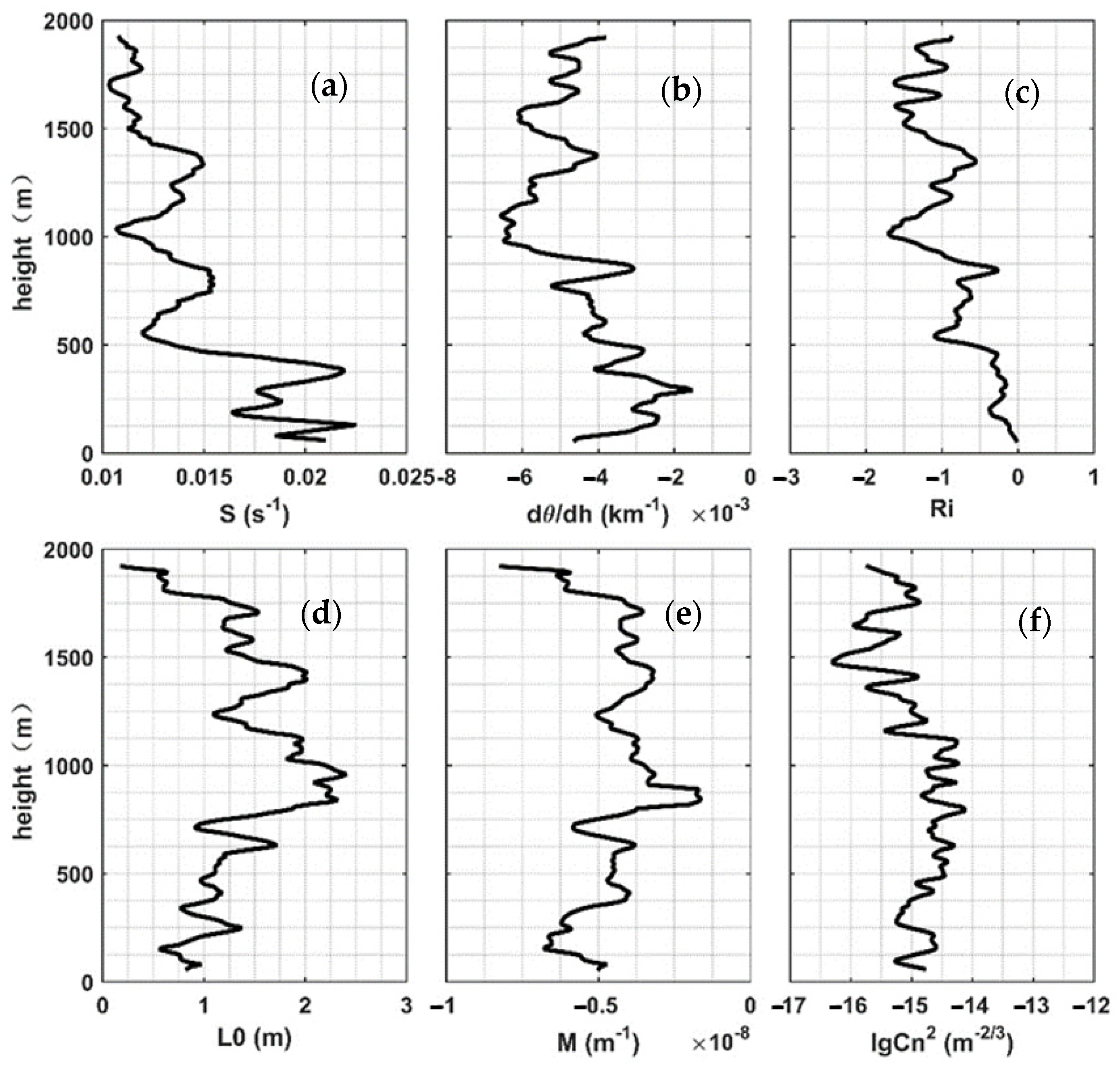
The monthly average profiles of C n 2 , as well as the profiles of possible influencing factors, are depicted in Figure 3. In this figure we have added the Richardson number, which is used to characterize the influence of temperature stratification and wind speed shear on the development of turbulence [48]. The height reported is the vertical distance above ground level in all figures of this paper. Furthermore, many studies have proved that the height of the offshore atmospheric boundary layer is below 2 km [49,50,51], so the maximum height of all profiles was fixed at 2 km in all panels. From Figure 3, we can see that the Richardson number profile has peaks when the wind shear and potential temperature gradient profile has large fluctuations at many altitudes. At the same height, the turbulent outer scale profile and the potential refractive index gradient profile also have maximum values, which can cause the appearance of a strong, turbulent, thin layer.

3.2. Setting Up of Contrast Experiments

In this study, the training data started from 15 November 2017, and finished on 14 December 2017 (30 days). The predicted data started from 15 December 2017, and finished on 30 December 2017 (16 days). Using random indices, all the training data were divided into the three portions involved, training data (0.6), validation data (0.25), and testing data (0.15). Seven variables, including height, temperature, relative humidity, pressure, wind speed, potential temperature gradient, and wind shear, are inputs of the BPNN architecture. Following the normalization process of the original data, the network iterated until it reached the maximum iterations (1000), or the performance reached the preset goals. Moreover, the popular Levenberg–Marquardt backpropagation algorithm was employed as the training function, which updated the weight and bias values according to Levenberg–Marquardt optimization [52,53]. The Levenberg–Marquardt backpropagation algorithm is often the fastest backpropagation algorithm and is highly recommended as a first-choice supervised algorithm, although it does require greater memory than other algorithms.
To better evaluate the performance of the BPNN approach, the HMNSP99 model for outer scale and the HAP model for a single parameter were used here to estimate C n 2 profiles. The potential temperature gradient and wind shear, which may be the cause of atmospheric turbulence, were added to the HMNSP99 model, making its estimation of turbulence intensity more credible. The C n 2 profile obtained by the BPNN approach in Figure 4 was predicted by using the trained network and input of basic meteorological data. C n 2 profiles derived from the HMNSP99 and HAP models were evaluated using basic meteorological parameters. In addition, there are C n 2 profiles measured by the radiosonde in the figure. Each figure contains four C n 2 profiles. Each method could obtain 32 profiles, for a total of 32 figures. Due to this large number, only six consecutive comparisons of the C n 2 profile are shown in Figure 4; and as can be seen, the C n 2 vertical distribution decreases sharply in the surface layer, mostly below 100 m. In the boundary layer, the C n 2 is generally in the order of 10−16 m−2/3. Both the BPNN approach and HMNSP99 model respect the variability and complexity of atmospheric turbulence better than the HAP model, but comparing the BPNN approach with the HMNSP99 model, it is clearly observed that the BPNN approach outperforms the HMNSP99 model in capturing the spatial evolution of C n 2 . The BPNN approach generally agrees with the measured values both in magnitude and trend. In contrast, the estimated values from the HMNSP99 model have relatively larger drift compared with radiosonde measurements at certain heights. The high variance may be attributed to a wider variety of atmospheric conditions, but overall, the estimated values of C n 2 profiles using the BPNN approach are more consistent with the measured values than the HMNSP99 model and HAP model.

3.3. Overall Approach to Performances

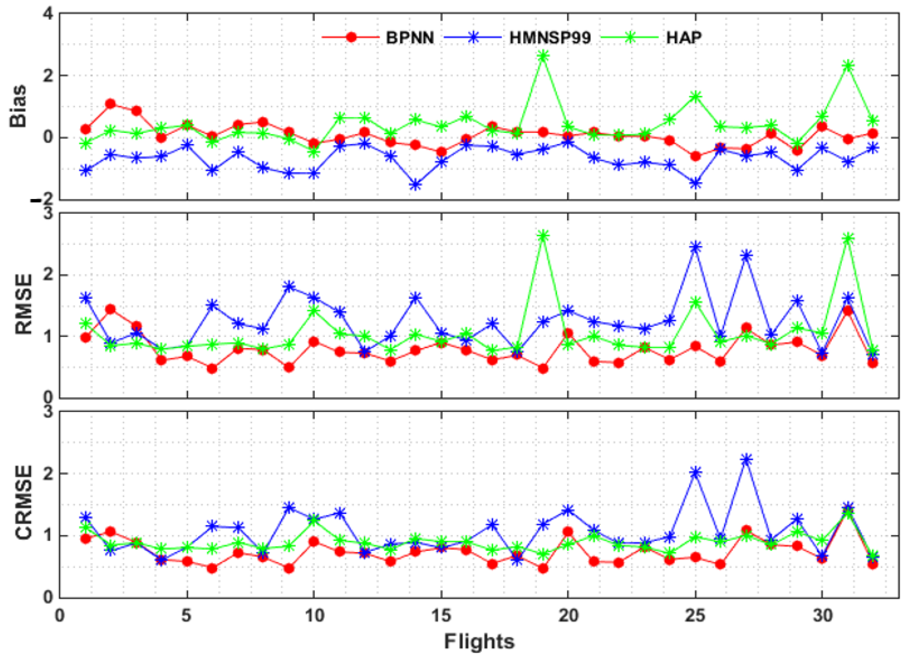
To quantify the calculation error of the above BPNN approach, HMNSP99 model and HAP model, the statistical results from individual flights of lg C n 2 between measurements and estimations are demonstrated in Figure 5. As shown in Figure 5, we used the BPNN approach, HMNSP99 model and HAP model to predict 32 C n 2 profiles. Then, the error analysis of the C n 2 profile predicted by each method and the measured C n 2 profile was carried out according to Equations (18)–(20). For each method, 32 error profiles were obtained for each, including the Bias, RMSE, and CRMSE. Then, each error profile was averaged to the height, with an average value obtained. A total of 32 error average values for each method were obtained. It is noted that the bias of the BPNN approach and the HAP model have no similarities except in a few flights. Most bias values calculated from the BPNN approach were between −0.5 and 0.5, but for the HMNSP99 model and HAP model, the maximum value exceeded −1 and 1, respectively. Compared with the results obtained by the HMNSP99 model and HAP model, we can observe that the BPNN approach had the lowest RMSE and CRMSE for 32 individual meteorological balloon flights. Most RMSE and CRMSE values obtained from the BPNN approach were below 1. At the same time, most RMSE and CRMSE values from the HAP model were slightly larger than the BPNN approach, and for the HMNSP99 model, half of the values were more than 1. In general, the BPNN approach had the highest stability and showed more reliable C n 2 profiles with better statistical results than the HMNSP99 and HAP models.
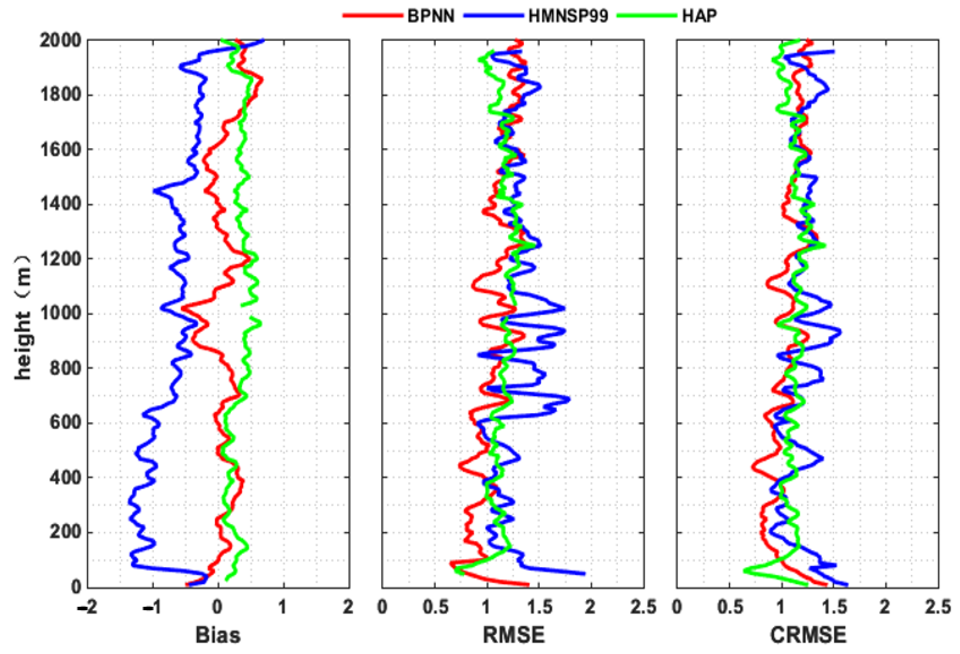
In addition, the overall statistics comparing the BNPP approach and the other models, derived from all 32 flights performed, are shown in Figure 6, with the vertical profiles of the bias, the RMSE and the CRMSE. According to Equations (18)–(20), N represents the amount of data in the horizontal direction for a couple ( X i , Y i ) at each precise height. In this section, we use N = 32 at each precise height. In detail, the bias, RMSE and CRMSE were calculated based on the C n 2 profiles with 10 m vertical resolution; then, a five-point moving average was applied to the final profiles. It can be seen from Figure 6 that the absolute values of the bias from the BPNN approach were lower than that from the HMNSP99 model and HAP model at most heights. Most bias values calculated from the BPNN approach were between −0.5 and 0.5 in the offshore atmospheric boundary layer. Note that for the HMNSP99 model there existed a larger bias value from 0 to 1500 m, and the maximum value exceeded −1. The RMSE and CRMSE of the BPNN approach were similar in value, and mainly smaller than 1.25 along the boundary layer. It is notable that the RMSE and CRMSE of the HMNSP99 model were larger than the BPNN approach, more noticeable between 500 and 1000 m. Moreover, almost all the RMSE and CRMSE of the HAP model fell between the BPNN approach and the HMNSP99 model results, which had a range from 1 to 1.25. In conclusion, the BPNN approach was more reliable than the HMNSP99 model and HAP model in reconstructing the strength of optical turbulence through individual and overall statistical analyses.
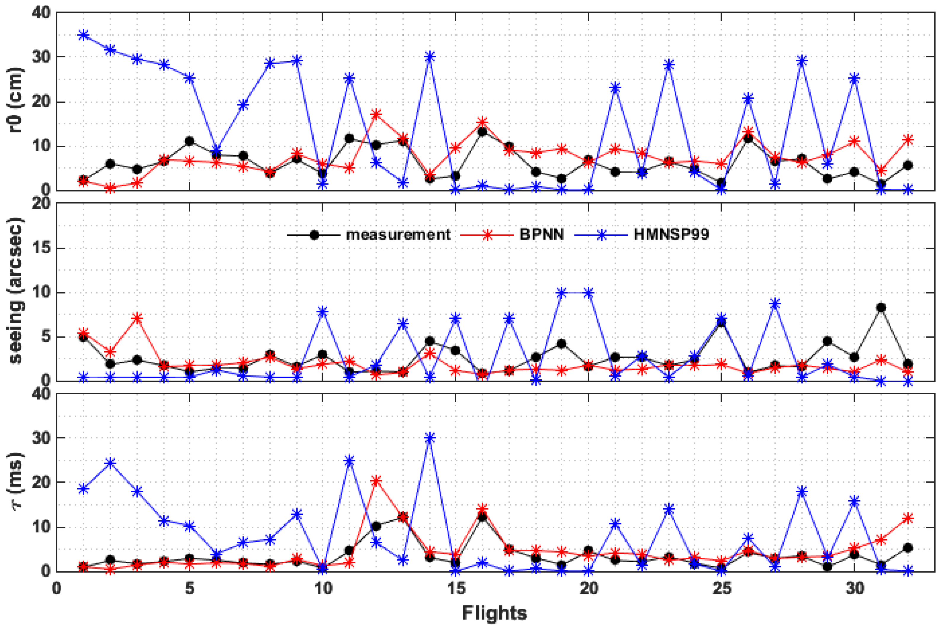
In this section, we focus attention on the ability of the BPNN approach to rebuild r 0 , ε, and τ 0 . The integrated astroclimatic parameters were obtained via C n 2 values measured by balloons and estimated by the BPNN approach and the HMNSP99 model. According to Equation (24), C n 2 is obtained through C T 2 . This formula is applicable to visible and near-infrared wavelengths. In order to maintain the consistency of the wavelength, the wavelength used in the calculation of the astroclimatic parameter was 0.55 microns. The results are shown in Figure 7. The BPNN approach provided more reasonable values, which were close to those measured by balloons, and compared with the results obtained by the BPNN approach, it can be seen that integrated astroclimatic parameters calculated from the HMNSP99 model fluctuated greatly. This is unreliable when reconstructing integrated astroclimatic parameters.

4. Conclusions

Optical turbulence has a serious impact on laser beam propagation through the atmosphere and on astronomical observations. Effective predictions of optical turbulence strength are significant for discussing atmospheric motion and transmission characteristics. In this paper, we proposed a simple and efficient technique to predict C n 2 profiles in the offshore atmospheric boundary layer. The proposed BPNN approach was demonstrated to estimate profiles in the offshore atmospheric boundary layer without any prior formula. From the analysis and comparison of the results with the HMNSP99 model and the HAP model, the corresponding conclusions are as follows:
(1) The BPNN approach identifies rules from big data without any assumptions, and so may be applied to a larger number of scenarios. Through continuous learning, the BPNN approach starts from basic meteorological parameters and obtains C n 2 profiles, avoiding the uncertainty and inaccuracy of model estimation.
(2) The BPNN approach has the highest computing precision compared with the HMNSP99 and HAP models. Most bias values calculated from the BPNN approach were between −0.5 and 0.5 in the offshore atmospheric boundary layer, and for the HMNSP99 model there existed a larger bias value from 0 to 1500 m, with the maximum value exceeding −1. The RMSE and CRMSE of the BPNN approach and the HMNSP99 model were mainly smaller than 1.25 and 1.75 along the boundary layer, respectively, and as for the HAP model, it had a range from 1 to 1.25.
(3) The profile modes of the offshore atmospheric boundary layer were induced using the BPNN approach. By calculating astroclimatic parameters, it was found that the BPNN approach provided more reasonable values, which are reliable when reconstructing integrated astroclimatic parameters.
Furthermore, the total training data were insufficient, and so the accuracy of the approach must be further improved.

Author Contributions

Conceptualization, M.X. and S.S.; software, M.X.; validation, formal analysis, M.X., S.S. and N.W.; investigation, M.X.; resources, G.S.; data curation, G.S. and Q.L.; writing—original draft preparation, M.X.; writing—review and editing, M.X.; visualization, M.X.; supervision, S.S., Y.H. and N.W.; project administration, funding acquisition, S.S. All authors have read and agreed to the published version of the manuscript.

Funding

This research was funded by the National Key Research and Development program under Grant 2018YFC0213102, the open project of Equipment Pre-research Fund under Grant 6142404180302, the National Natural Science Foundation of China under Grant 41475024, and the National Natural Science Foundation of China under Grant 42027804.

Institutional Review Board Statement

Not applicable.

Informed Consent Statement

Not applicable.

Data Availability Statement

The data are contained within the article.

Acknowledgments

We thank Xiaoquan Song from the Ocean University of China for comments and suggestions. In addition, the authors would like to thank Shiyong Shao and Ningquan Weng for their patient help and guidance.

Conflicts of Interest

The authors declare no conflict of interest.

References

  1. Stull, R. An Introduction To Boundary Layer Meteorology; Kluwer Academic Publishers: Norwell, MA, USA, 1988; Volume 13, pp. 1–2. [Google Scholar]
  2. Andrews, L.; Phillips, R. Laser Beam Propagation through Random Media; SPIE Optical Engineering Press: Bellingham, DC, USA, 2005. [Google Scholar] [CrossRef]
  3. Wang, Y.; Basu, S. Utilizing the Kantorovich metric for the validation of optical turbulence predictions. Opt. Lett. 2016, 41, 4008–4011. [Google Scholar] [CrossRef]
  4. Song, T.; Cai, Z.; Liu, Y.; Zhao, M.; Fang, Y.; Zhang, X.; Wang, J.; Li, X.; Song, Q.; Du, Z. Daytime optical turbulence profiling with a profiler of the differential solar limb. Mon. Not. R. Astron. Soc. 2020, 499, 1909–1917. [Google Scholar] [CrossRef]
  5. Shen, H.; Yu, L.; Jing, X.; Tan, F. Method for Measuring the Second-Order Moment of Atmospheric Turbulence. Atmosphere 2021, 12, 564. [Google Scholar] [CrossRef]
  6. Chabé, J.; Aristidi, E.; Ziad, A.; Lantéri, H.; Fanteï-Caujolle, Y.; Giordano, C.; Borgnino, J.; Marjani, M.; Renaud, C. PML: A generalized monitor of atmospheric turbulence profile with high vertical resolution. Appl. Opt. 2020, 59, 7574–7584. [Google Scholar] [CrossRef] [PubMed]
  7. Shikhovtsev, A.; Kiselev, A.; Kovadlo, P.; Kolobov, D.; Lukin, V.; Tomin, V. Method for Estimating the Altitudes of Atmospheric Layers with Strong Turbulence. Atmos. Ocean. Opt. 2020, 33, 295–301. [Google Scholar] [CrossRef]
  8. Vernin, J.; Barletti, R.; Ceppatelli, G.; Paternò, L.; Righini, A.; Speroni, N. Optical remote sensing of atmospheric turbulence: A comparison with simultaneous thermal measurements. Appl. Opt. 1979, 18, 243–247. [Google Scholar] [CrossRef]
  9. Anand, N.; Sunilkumar, K.; Satheesh, S.; Moorthy, K.K. Entanglement of near-surface optical turbulence to atmospheric boundary layer dynamics and particulate concentration: Implications for optical wireless communication systems. Appl. Opt. 2020, 59, 1471–1483. [Google Scholar] [CrossRef]
  10. Kaimal, J.C.; Wyngaard, J.C. The Kansas and Minnesota experiments. Bound.-Layer Meteorol. 1990, 50, 31–47. [Google Scholar] [CrossRef]
  11. Van Iersel, M.; Paulson, D.A.; Wu, C.; Ferlic, N.A.; Rzasa, J.R.; Davis, C.C.; Walker, M.; Bowden, M.; Spychalsky, J.; Titus, F. Measuring the turbulence profile in the lower atmospheric boundary layer. Appl. Opt. 2019, 58, 6934–6941. [Google Scholar] [CrossRef]
  12. Coulman, C.E. A quantitative treatment of solar ‘seeing’, II. Sol. Phys. 1974, 34, 491–506. [Google Scholar] [CrossRef]
  13. Coulman, C.E. Vertical profiles of small-scale temperature structure in the atmosphere. Bound.-Layer Meteorol. 1973, 4, 169–177. [Google Scholar] [CrossRef]
  14. Bufton, J. Correlation of Microthermal Turbulence Data with Meteorological Soundings in the Troposphere. J. Atmos. Sci. 1973, 30, 83–87. [Google Scholar] [CrossRef]
  15. Bufton, J. Comparison of Vertical Profile Turbulence Structure with Stellar Observations. Appl. Opt. 1973, 12, 1785–1793. [Google Scholar] [CrossRef]
  16. Azouit, M.; Vernin, J. Optical Turbulence Profiling with Balloons Relevant to Astronomy and Atmospheric Physics. Publ. Astron. Soc. Pac. 2005, 117, 536–543. [Google Scholar] [CrossRef]
  17. McHugh, J.; Jumper, G.; Chun, M. Balloon Thermosonde Measurements over Mauna Kea and Comparison with Seeing Measurements. Publ. Astron. Soc. Pac. 2008, 120, 1318–1324. [Google Scholar] [CrossRef]
  18. Miller, M.; Zieske, P. Turbulence Environment Characterization; Avco-Everett Research Lab.: Everett, MA, USA, 1979; 135p. [Google Scholar]
  19. Good, R.E.; Beland, R.R.; Murphy, E.A.; Brown, J.H.; Dewan, E.M. Atmospheric models of optical turbulence. Proc. SPIE 1988, 928, 165–186. [Google Scholar] [CrossRef]
  20. Jumper, G.; Beland, R. Progress in the Understanding and Modeling of Atmospheric Optical Turbulence. In Proceedings of the 31st Plasmadynamics and Lasers Conference, Denver, CO, USA, 19–22 June 2000. [Google Scholar] [CrossRef]
  21. Beland, R.R.; Brown, J.H. A deterministic temperature model for stratospheric optical turbulence. Phys. Scr. 1988, 37, 419–423. [Google Scholar] [CrossRef]
  22. Hufnagel, R.; Stanley, N. Modulation Transfer Function Associated with Image Transmission through Turbulent Media. JOSA 1964, 54, 52–60. [Google Scholar] [CrossRef]
  23. Tatarski, V.L. Wave Propagation in a Turbulent Medium; Silverman, R.A., Translator; McGraw-Hill: New York, NY, USA, 1961; Volume 134, 285p. [Google Scholar] [CrossRef]
  24. Felton, B.; Alliss, R. Improved climatological characterization of optical turbulence for free-space optical communications. In Proceedings of the SPIE Optical Engineering + Applications, San Diego, CA, USA, 21–25 August 2011; Volume 8162. [Google Scholar] [CrossRef]
  25. Kovadlo, P.G.; Lukin, V.P.; Shikhovtsev, A.Y. Development of the Model of Turbulent Atmosphere at the Large Solar Vacuum Telescope Site as Applied to Image Adaptation. Atmos. Ocean. Opt. 2019, 32, 202–206. [Google Scholar] [CrossRef]
  26. Zhang, R.; Jing, J.; Tao, J.; Hsu, S.C.; Wang, G.; Cao, J.; Lee, C.S.L.; Zhu, L.; Chen, Z.; Zhao, Y.; et al. Chemical characterization and source apportionment of PM2.5 in Beijing: Seasonal perspective. Atmos. Chem. Phys. 2013, 13, 7053–7074. [Google Scholar] [CrossRef] [Green Version]
  27. Suárez Gómez, S.; Gonzalez, C.; Alonso, E.; Santos, J.D.; Rodríguez, M.; Morris, T.; Osborn, J.; Basden, A.; Bonavera, L.; González, J.; et al. Experience with Artificial Neural Networks Applied in Multi-object Adaptive Optics. Publ. Astron. Soc. Pac. 2019, 131, 108012. [Google Scholar] [CrossRef]
  28. Lohani, S.; Glasser, R.T. Turbulence correction with artificial neural networks. Opt. Lett. 2018, 43, 2611–2614. [Google Scholar] [CrossRef]
  29. Pelliccioni, A.; Tirabassi, T. Air dispersion model and neural network: A new perspective for integrated models in the simulation of complex situations. Environ. Model. Softw. 2006, 21, 539–546. [Google Scholar] [CrossRef]
  30. Tracey, B.D.; Duraisamy, K.; Alonso, J.J. A Machine Learning Strategy to Assist Turbulence Model Development. In Proceedings of the 53rd AIAA Aerospace Sciences Meeting, Kissimmee, FL, USA, 5–9 January 2015. [Google Scholar]
  31. Wang, Y.; Basu, S. Using an artificial neural network approach to estimate surface-layer optical turbulence at Mauna Loa, Hawaii. Opt. Lett. 2016, 41, 2334–2337. [Google Scholar] [CrossRef]
  32. Su, C.; Wu, X.; Luo, T.; Wu, S.; Qing, C. Adaptive niche-genetic algorithm based on backpropagation neural network for atmospheric turbulence forecasting. Appl. Opt. 2020, 59, 3699–3705. [Google Scholar] [CrossRef]
  33. Rumelhart, D.E.; Hinton, G.E.; Williams, R.J. Learning representations by back-propagating errors. Nature 1986, 323, 533–536. [Google Scholar] [CrossRef]
  34. Tatarski, V.I.; Silverman, R.A.; Chako, N. Wave Propagation in a Turbulent Medium. Phys. Today 1961, 14, 46. [Google Scholar] [CrossRef]
  35. Beland, R.R. Propagation through atmospheric optical turbulence. Atmos. Propag. Radiat. 1993, 2, 157–232. [Google Scholar]
  36. Han, Y.; Wu, X.; Luo, T.; Qing, C.; Yang, Q.; Jin, X.; Liu, N.; Wu, S.; Su, C. New statistical model based on first radiosonde turbulence observation over Lhasa. J. Opt. Soc. Am. A 2020, 37, 995–1001. [Google Scholar] [CrossRef]
  37. Ruggiero, F.H.; Debenedictis, D.A. Forecasting optical turbulence from mesoscale numerical weather prediction models. In Proceedings of the DoD High Performance Modernization Program Users Group Conference; Austin, Texas, USA: 10–14 June 2002.
  38. Andrews, L.C.; Phillips, R.L.; Wayne, D.; Leclerc, T.; Sauer, P.; Crabbs, R.; Kiriazes, J. Near-ground vertical profile of refractive-index fluctuations. In Proceedings of the SPIE Defense, Security, and Sensing, Orlando, FL, USA, 13–17 April 2009. [Google Scholar]
  39. Masciadri, E.; Lascaux, F.; Fini, L. MOSE: Operational forecast of the optical turbulence and atmospheric parameters at European Southern Observatory ground-based sites—I. Overview and vertical stratification of atmospheric parameters at 0–20 km. Mon. Not. R. Astron. Soc. 2013, 436, 1968–1985. [Google Scholar] [CrossRef] [Green Version]
  40. Roddier, F.; Gilli, J.M.; Lund, G. On the origin of speckle boiling and its effects in stellar speckle interferometry. J. Opt. 2000, 13, 263. [Google Scholar] [CrossRef]
  41. Fried, D.L. Optical Resolution through a Randomly Inhomogeneous Medium for Very Long and Very Short Exposures. J. Opt. Soc. Am. 1966, 56, 1372–1379. [Google Scholar] [CrossRef]
  42. Shao, S.; Qin, F.; Liu, Q.; Xu, M.; Cheng, X. Turbulent Structure Function Analysis Using Wireless Micro-Thermometer. IEEE Access 2020, 8, 123929–123937. [Google Scholar] [CrossRef]
  43. Lawrence, R.S.; Ochs, G.R.; Clifford, S.F. Measurements of atmospheric turbulence relevant to optical propagatian. J. Opt. Soc. Am. 1970, 60, 826–830. [Google Scholar] [CrossRef]
  44. Tatarskii, V.I. The Effects of the Turbulent Atmosphere on Wave Propagation; Israel Program for Scientific Translations: Jerusalem, Israel, 1971. [Google Scholar]
  45. Xiaoqing, W.U.; Qiguo, T.; Peng, J.; Bo, C.; Qing, C.; Jun, C.A.I.; Xinmiao, J.I.N.; Hongyan, Z. A new method of measuring optical turbulence of atmospheric surface layer at Antarctic Taishan Station with ultrasonic anemometer. Adv. Polar Sci. 2015, 26, 305. [Google Scholar] [CrossRef]
  46. Qing, C.; Wu, X.; Li, X.; Zhu, W.; Qiao, C.; Rao, R.; Mei, H. Use of weather research and forecasting model outputs to obtain near-surface refractive index structure constant over the ocean. Opt. Express 2016, 24, 13303–13315. [Google Scholar] [CrossRef] [PubMed]
  47. Cai, J.; Li, X.B.; Zhan, G.W.; Wu, P.F.; Xu, C.Y.; Qing, C.; Wu, X.Q. A new model for the profiles of optical turbulence outer scale and Cn2 on the coast. Wuli Xuebao/Acta Phys. Sin. 2018, 67, 014206. [Google Scholar] [CrossRef]
  48. Ellrod, G.P.; Lester, P.F.; Ehernberger, L.J. Clear Air Turbulence. In Encyclopedia of Atmospheric Sciences; Holton, J.R., Ed.; Academic Press: Oxford, UK, 2003; pp. 393–403. [Google Scholar] [CrossRef]
  49. McGrath-Spangler, E.L.; Denning, A.S. Global seasonal variations of midday planetary boundary layer depth from CALIPSO space-borne LIDAR. J. Geophys. Res. Atmos. 2013, 118, 1226–1233. [Google Scholar] [CrossRef]
  50. Sathyanadh, A.; Prabhakaran, T.; Patil, C.; Karipot, A. Planetary boundary layer height over the Indian subcontinent: Variability and controls with respect to monsoon. Atmos. Res. 2017, 195, 44–61. [Google Scholar] [CrossRef]
  51. Sudeepkumar, B.L.; Babu, C.A.; Varikoden, H. Atmospheric boundary layer height and surface parameters: Trends and relationships over the west coast of India. Atmos. Res. 2020, 245, 105050. [Google Scholar] [CrossRef]
  52. Levenberg, K. A method for the solution of certain non-linear problems in least squares. Q. Appl. Math. 1944, 2, 164–168. [Google Scholar] [CrossRef] [Green Version]
  53. Marquardt, D.W. An Algorithm for Least-Squares Estimation of Nonlinear Parameters. J. Soc. Ind. Appl. Math. 1963, 11, 431–441. [Google Scholar] [CrossRef]
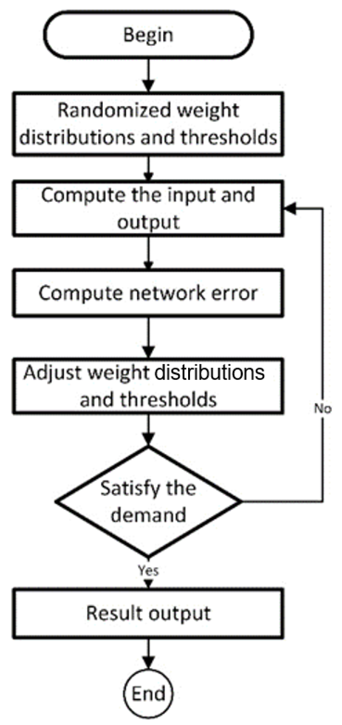
Figure 1. Flowchart of the BP neural network.
Applsci 11 08523 g001
Figure 2. Launching a balloon-borne radiosonde.
Applsci 11 08523 g002
Figure 3. Average profiles of (a) wind shear, (b) potential temperature gradient, (c) Richardson number, (d) outer scale, (e) potential refractive index gradient and (f) C n 2 measured by all samples of balloon-borne radiosondes.
Applsci 11 08523 g003
Figure 4. Vertical profiles of C n 2 from the radiosonde, BP neural network, HMNSP99 model and HAP model.
Applsci 11 08523 g004
Figure 5. Statistical analysis of lg C n 2 calculated by the BPNN approach, HMNSP99 model and HAP model for all samples of individual meteorological balloons.
Applsci 11 08523 g005
Figure 6. Overall statistical analysis of lg C n 2 profiles of 32 balloon samples.
Applsci 11 08523 g006
Figure 7. Comparison of integrated astroclimatic parameters between measurement, the BPNN approach and the HMNSP99 model.
Applsci 11 08523 g007
Publisher’s Note: MDPI stays neutral with regard to jurisdictional claims in published maps and institutional affiliations.