Article

Physically Consistent Scar Tissue Dynamics from Scattered Set of Data: A Novel Computational Approach to Avoid the Onset of the Runge Phenomenon

1
Translational Neural Engineering Area, The BioRobotics Institute and Department of Excellence in Robotics and Artificial Intelligence, Sant’Anna School of Advanced Studies, Piazza Martiri della Libertà, 33, 56127 Pisa, Italy
2
Institut de Neurociències, Department of Cell Biology, Physiology and Immunology, Universitat Autònoma de Barcelona, and CIBERNED, 08193 Bellaterra, Spain
3
Bertarelli Foundation Chair in Translational Neural Engineering, Center for Neuroprosthetics and Institute of Bioengineering, Ecole Polytechnique Federale de Lausanne, Rte Cantonale, 1015 Lausanne, Switzerland
*
Author to whom correspondence should be addressed.
Appl. Sci. 2021, 11(18), 8568; https://doi.org/10.3390/app11188568
Submission received: 3 July 2021 / Revised: 8 September 2021 / Accepted: 10 September 2021 / Published: 15 September 2021

Abstract

:
The foreign body reaction is a complex biological process leading to the insulation of implanted artificial materials through a capsule of scar tissue. In particular, in chronic implantations of neural electrodes, the prediction of the scar tissue evolution is crucial to assess the implant reliability over time. Indeed, the capsule behaves like an increasing insulating barrier between electrodes and nerve fibers. However, no explicit and physically based rules are available to computationally reproduce the capsule evolution. In addition, standard approaches to this problem (i.e., Vandermonde-based and Lagrange interpolation) fail for the onset of the Runge phenomenon. More specifically, numerical oscillations arise, thus standard procedures are only able to reproduce experimental detections while they result in non physical values for inter-interval times (i.e., times before and after experimental detections). As a consequence, in this work, a novel framework is described to model the evolution of the scar tissue thickness, avoiding the onset of the Runge phenomenon. This approach is able to provide novel approximating functions correctly reproducing experimental data ( R 2 0.92 ) and effectively predicting inter-interval detections. In this way, the overall performances of previous approaches, based on phenomenological fitting polynomials of low degree, are improved.

1. Introduction

Peripheral neural interfaces are high tech devices able to record neural signals and evoke neural activity through the stimulation of axonal clusters. Different types of intraneural electrodes have been designed [1,2,3,4] to be directly inserted within peripheral nerves or to be implanted through microneedles [5,6,7], while other types of regenerative neural interfaces were studied [1,8,9] to exploit the axonal regeneration [10,11,12,13]. In particular, intraneural interfaces were able to provide selective recording and stimulation, keeping their overall invasiveness low. Unfortunately, as the foreign body reaction (FBR) affects the interaction between living tissue and synthetic materials [14,15], similarly it affects the interaction between the peripheral nervous tissue [16,17,18,19,20,21,22,23] and intraneural interfaces [24,25,26], resulting in the formation of a tissue capsule [27,28] around the implanted structures.
Several studies explored the FBR details describing a first phase related to the adsorption of blood and plasma proteins (e.g., fibrinogen, fibronectin, albumin and antibodies) to the implant surface [29,30]. Therefore, a second phase was described where the adsorbed protein layer promoted monocyte and leukocyte extravasation, attraction and adhesion to the surface, together with the coagulation cascade [31,32,33]. Then, a sort of matrix of fibrin was found to attract circulating leukocytes and local macrophages around the surface of the implanted material under the chemical attraction of chemokines [32,34]. Furthermore, it was described as the way extravasated monocytes differentiate to macrophages and fuse together to form multinucleated foreign body giant cells (FBGCs). These cells started releasing further inflammatory cytokines, boosting the inflammatory response through a positive feedback mechanism [35,36]. Then, it was described as myofibroblasts triggered a massive secretion of extracellular matrix (ECM) components [15,27,37]. Finally, at the end of the whole process, the scar tissue capsule was found to be impermeable to the nonspecific immune system and to many chemicals [14,15,27].
Both the complexity of the FBR [14,15,27,28,29,30,31,32,33,34,35,36,37,38] and the unclear relationship between the physical properties of peripheral nerves [7,39,40,41,42,43,44,45,46,47,48] and the amount of scar tissue production makes a reliable prediction of the capsule thickness a challenging task.
Some previous studies explored the evolution of the FBR caused by intraneural electrodes longitudinally implanted (e.g., LIFE electrodes [49,50]) in the rat peripheral nerves, while others explored the cellular composition and the thickness of the fibrotic capsule in a time span ranging from 1 day to 8 months [51,52]. These investigations revealed that the contacts between the nerve fibers and the electrode active sites were partially lost because of the outgrowth of the encapsulating tissue. In particular, the increase of the scar capsule was directly related to the increase of the electrical impedance, resulting first in the decrease of the signal to noise ratio [53] and possibly in a sensible drop of registration and stimulation capabilities [36,54].
Therefore, a correct and quantitative assessment of the capsule thickness over time is crucial information to improve the design of intraneural interfaces as well as their implantation technique. However, the development of the FBR involves several interrelated complex processes [14,15,27,28,29,30,31,32,33,34,35,36,37,38] which are partially hidden since their explicit and physically based rules are not known in all details.
Nevertheless, it is a pressing issue to investigate whether computational strategies are able to reproduce the scar tissue evolution, making sense of the huge complexity of the underlying phenomena. In particular, a suitable trade off between light computational models and physically meaningful dynamics has to be found. Under these constraints the identification of a reliable procedure to reproduce the scar capsule thickness was not foreseen and standard numerical approaches [55,56] fail. In addition, if the experimental sets of data are small, with experimental time points which are closer together, ill-conditioned systems could arise, further increasing the complexity of the problem.
As a consequence, in this work, a novel numerical procedure was provided to reproduce and predict the evolution of the scar capsule mean thickness, starting from a whole set of scattered experimental data with low cardinality [57]. More specifically, two classic approaches, fully exploiting experimental data and optimizing standard metrics, are first presented for benchmark. Therefore, the onset of the Runge phenomenon, affecting their ability to reproduce data through high-degree polynomial functions [55,56], was explored. Since the optimization of standard metrics was not able to avoid huge errors in predictions due to the onset of this numerical phenomenon, a novel approach was proposed to overcome previous standard models by optimizing the parametrization of the scar thickness evolution over time. Finally, a novel metric was provided to better investigate the suitability of potential candidate functions in reproducing the experimental data set.

2. Methods

Experiments were performed to measure the thickness of the scar tissue capsule around polymeric stripes implanted within in vivo mice, as explained in detail in [57]. A standard procedure was used to evaluate the microstructure of the nerve and the thickness of the tissue capsule around the implant, as explained in [58]. More specifically, nerve segments were postfixed and embedded in epon resin, while semithin sections (0.5 μm thick) were stained (toluidine blue) and investigated by light microscopy. A representative section from the central part of the implant in the nerve was chosen for each animal, while the thickness of the scar capsule was computed as the distance between each side of the implant and the closest myelinated axon using ImageJ software (U.S. National Institutes of Health, Bethesda, MD, USA). In particular, the scar thickness was assessed at 1, 2 and 4 days and 4, 8, 16 and 32 weeks post insertion [57]. This experimental approach resulted in a scattered numerical subset s ˜ ( t ) = { s ( t 0 ) , , s ( t 8 ) } with low cardinality. First, a well known standard approach (i.e., Vandermonde-based polynomial interpolation [59,60]) was used to approximate the continuous evolution of the thickness over time from scattered data. More specifically, the basis of polynomials { 1 , t , t n } was chosen and the coefficients of the interpolating polynomial function were found through the solution of the system:
s ˜ ( t ) = V ( t ) a
where s ˜ ( t ) was the experimental data vector, while V ( t ) was the classic Vandermonde matrix defined as:
V ( t ) = 1 t t n 2 t n 1 1 t t n 2 t n 1 1 t t n 2 t n 1 1 t t n 2 t n 1
while a = { a 0 , a 1 , , a n } T was the vector of numeric coefficients. Therefore, once the system in Equation (1) was inverted, the interpolating function was written as:
q n ( t ) = i = 0 n 1 a i t i
where n = 9 was the number of data points known through experiments. A second standard approach, fully exploiting the experimental information over time, was implemented through the Lagrange interpolation polynomials [59,60], which were defined as:
g n ( t ) = j = 0 n 1 s ( t j ) k = 0 , k j n t t k t j t k
where n was, again, the number of experimental points. Once developed, this function was written as:
g n ( t ) = j = 0 n 1 x j t j
where x i R were numerical coefficients related through Equation (4) to s ( t j ) . However, since the cardinality of the known set of data points was small, supplementary points were added to improve the quality of the interpolation process.
More specifically, the last two points of the experimental time detections were used to obtain a further middle time point through
t ω = [ t n + t n 1 ] / 2
where, n = 9 was the actual cardinality of the experimental data set. The thickness related to this further time point was found as:
s ( t ω ) = [ s ( t n 1 ) + s ( t n ) ] / 2
In the last part of the curve a steady state was guessed. After the first application of Equations (6) and (7) the cardinality of the set of points was increased by one unit (i.e., n = 9 + 1 = 10 ). Similarly, this procedure was iteratively performed two times in order to add two and three further points to the initial data set. In other words, each novel set of points was obtained from the previous one by adding one further point, so the cardinality of the novel sets was n = 9 + 2 = 11 (second iteration) and 9 + 3 = 12 (third iteration), respectively.
Since more data points were exploitable, higher degree interpolant polynomials were used. In addition, these polynomials were recursively connected through the Neville’s formula:
g n ( t ) = ( t t j ) g n 1 , j ( t ) ( t t i ) g n 1 , i ( t ) t i t j
where i , j N were both i , j < n , and i j were two different integers. In addition, g n ( t ) was the n-th order function, interpolating the data points at t 0 , t 1 , , t n , while g n 1 , i ( t ) was the n-1-th order approximate function, interpolating the data points at t 0 , t 1 , , t i 1 , t i + 1 , , t n . Moreover, the previous approaches were heavily affected by the number of the experimental points which were available for the reconstruction procedure. As a consequence, a novel approach was proposed to disentangle the reconstruction of the thickness over time from the available experimental information. More specifically, novel functions J H S 0 ( t ) , J H S 1 ( t ) , J H S 2 ( t ) , J H S n ( t ) were introduced and defined as:
J H S ξ ( t ) = ( 2 ξ + 1 ) ! ! ( 2 ξ + 1 ) ! d ξ d t ξ [ ( t ξ + 2 + t + 1 ) ξ ξ + 1 ]
where ξ N was a natural number. The approximating candidate functions were then expressed as:
w m ( t ) = i = 0 m H m , i J H S i ( t )
where H m , i R were numeric coefficients related to the summation index m N . These coefficients, which were now not related to the amount of experimental information, were condensed into the H m vector. In this work, for the sake of simplicity, only the functions related to values of m ranging from 0 to 5 were explored (see Appendix A about how to build these functions).
More specifically, all the new functions in Equation (10) were used to numerically reproduce (nonlinear least squares method, Levemberg–Marquardt algorithm with all starting guess set to be zero) the evolution of the scar capsule thickness over time in MATLAB (MathWorks, Inc., Portola Valley, CA, USA), through the optimization of the numeric coefficients of the H m vector.
Furthermore, to quantify the intensity of the Runge phenomenon for each approximating function, the following dimensionless metric was used:
Λ f = l n m a x { f ( t ) } m i n { f ( t ) } m a x { s ˜ ( t ) } m i n { s ˜ ( t ) }
where f was each of the previous approximating function (i.e., g 9 ( t ) , g 10 ( t ) , g 11 ( t ) , g 12 ( t ) , q 9 ( t ) , w 1 ( t ) , w 2 ( t ) , w 3 ( t ) , w 4 ( t ) , w 5 ( t ) ) and m a x { s ( t ) ˜ } and m i n { s ( t ) ˜ } were the maximum and the minimum values of the experimental thickness.
Finally, to figure out the overall suitability of each candidate function, the following dimensionless metric was introduced:
I f = k R 2 d f · ( S S E + 1 ) · Λ f
where k = 10 4 [μm] was a dimensional constant, R 2 was the square of the multiple correlation coefficient, while SSE was the value of the sum of squared errors and d f = m a x { f ( t ) } m i n { f ( t ) } [ μ m ] was the difference between the maximum and minimum values of the approximating function over time.

3. Results

The reconstruction of a continuous evolution of the scar tissue thickness from a small scattered set of experimental data through Equation (1) involved the use of the Vandermonde matrix in Equation (2). However, this matrix was badly conditioned (Figure 1a) and resulted in a polynomial function (Equation (3)) which was fully characterized by the elements of the a vectors (see Table 1). This polynomial was able to exactly reproduce experimental detections (i.e., R 2 = 1 , S S E = 0 ), even if its evolution greatly differed from experimental points for inter-interval time values. In particular, the maximum difference between predicted values and expected ones was about 1.62 × 10 8 at t = 4839 h (Figure 1b).
Trying to improve this approach, the experimental times were normalized over the maximum time, then all the normalized experimental times ranged between 0 and 1. In this second case, the Vandermonde matrix was better conditioned (Figure 1c), but the function was still affected by the same numerical error in predictions (the maximum error was the same) even if scaled on abscissas (in this case the normalized time was 0.897 ), as shown in Figure 1d.
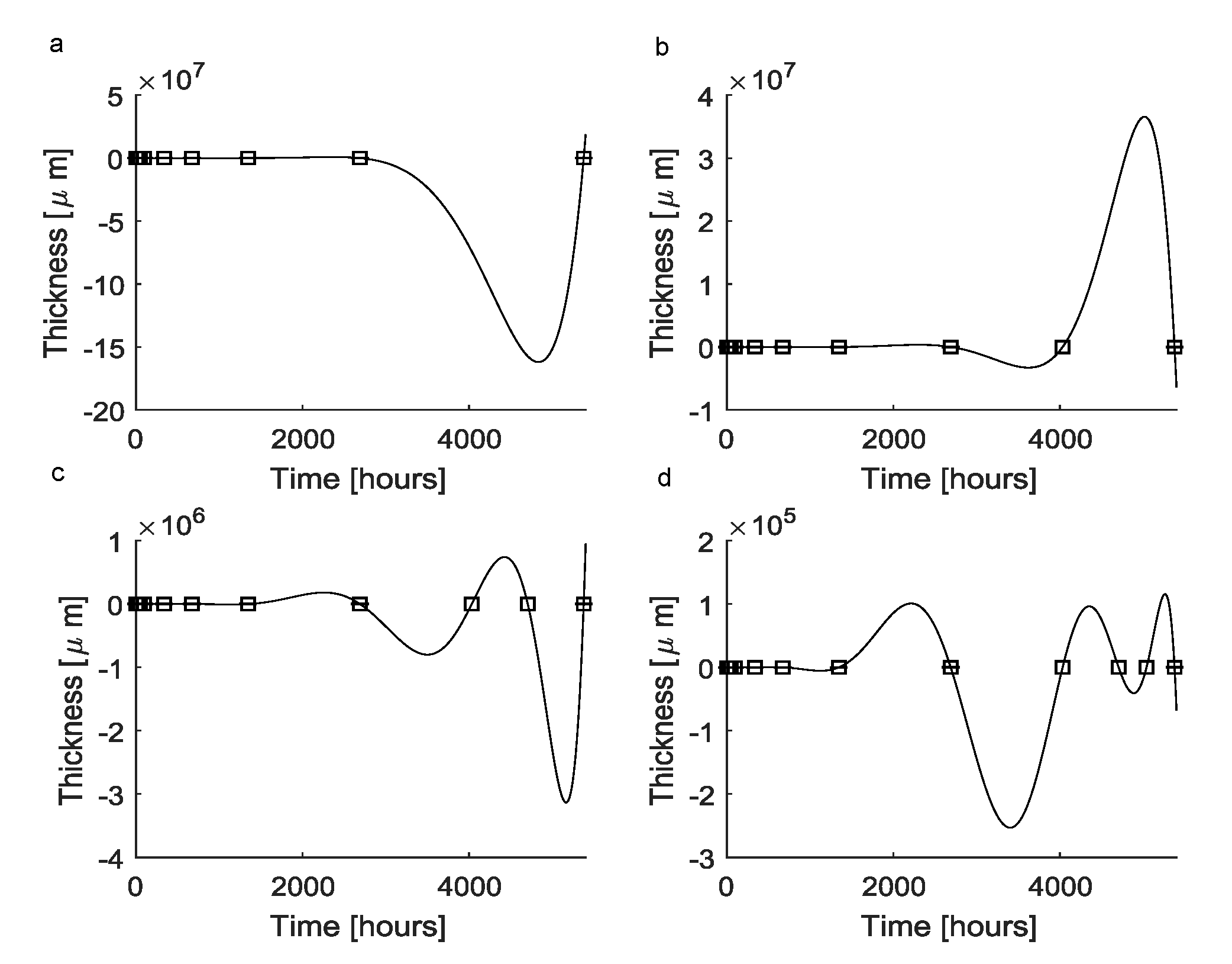
Since the classic Vandermonde approach failed, a second approach was implemented to find a continuous function reproducing the scar tissue dynamics. First, Equation (4) was used to obtain a polynomial approximating function g 9 ( t ) (Figure 2a), which, by definition, was able to exactly reproduce all experimental points ( R 2 = 1 , S S E = 0 ). This function, which was expressed through Equation (5), was fully characterized by the x vector whose coefficients are equals to those of the a vector resulting from the previous approach (see Table 1). In particular, since the Runge phenomenon arose, at t = 4838 h the predicted thickness of the scar capsule was s ( 4838 ) = 1.62 × 10 8 μm.
To improve this standard approach, some further time points were added through the use of Equations (6) and (7). In particular, as a result of the first iteration, the time point t = 4032 h was added and the predicted thickness was s(4032) = 47.039 μm. By adding this time point to the experimental data set (i.e., new total number of detections n = 9 + 1 = 10 ), the resulting approximating function g 10 ( t ) (Figure 2b) was characterized by the x vector (see Table 2, column 1). In this case, at t = 5016 h, the predicted thickness was s ( 5016 ) = 3.656 × 10 7 μm because of the arising numerical oscillations.
Again, by iterating this process, an additional time point was created at t = 4704 , while the predicted thickness was s ( 4704 ) = 47.025 μm. The coefficients of the approximating function g 11 ( t ) are shown in Table 2, column 2, while the maximum thickness value was s ( 5167 ) = 3.134 × 10 6 μm at t = 5167 due to the influence of the Runge phenomenon. Finally, by iterating the previous procedure once more, an additional time point was created at t = 5040 h, the predicted thickness was s ( 5040 ) = 47.018 μm and the numerical coefficients characterizing the candidate function g 12 ( t ) are shown in Table 2, column 3. Moreover, in this case, the Runge phenomenon arose leading to a prediction of s ( 3397 ) = 2.53 × 10 5 μm at t = 3397 h. It is worthy to note that for all the previous candidate functions g 10 ( t ) , g 11 ( t ) , g 12 ( t ) , by definition, standard metrics values were R 2 = 1 , S S E = 0 .
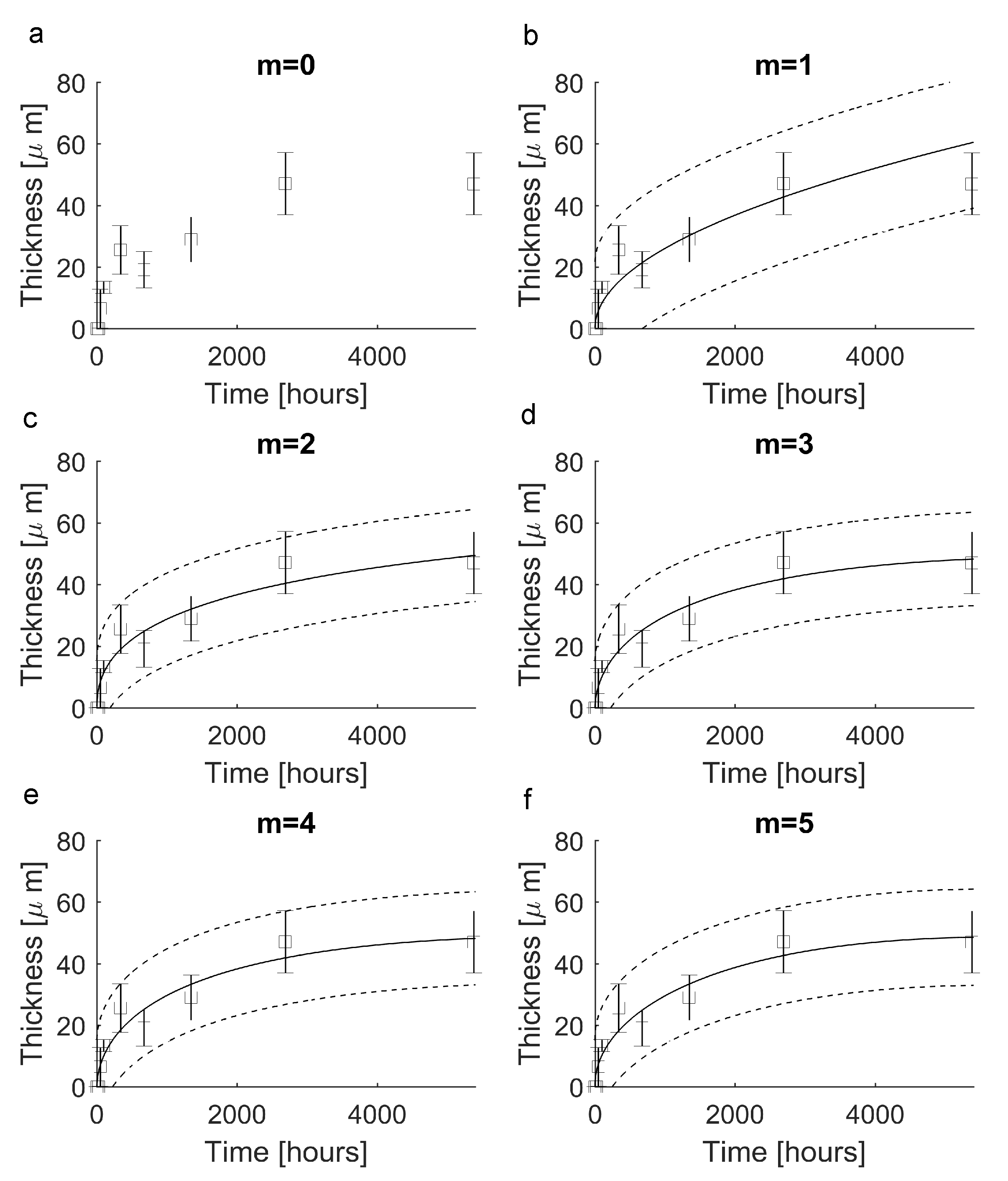
In order to provide a novel way to reconstruct a continuous evolution from the experimental data set, Equation (10) was tested for m = 0 , , 5 . In all cases, the elements of each H m vector are shown in Figure 3 (lines 0–5). In particular, for m = 0 , the function was constant ( H 0 , 0 = 22.51 ) and resulted in nonnegligible errors (i.e., S S E = 4181 , see Figure 4a). For m = 1 , instead, the function w 1 ( t ) was able to follow the experimental evolution and resulted in R 2 = 0.866 , S S E = 347.3 (Figure 4b). Similarly, for m = 2 , the function w 2 ( t ) led to R 2 = 0.9195 , S S E = 208.9 (Figure 4c), while for m = 3 and then for the candidate function w 3 ( t ) , the values of standard metrics were R 2 = 0.9197 , S S E = 208.4 (Figure 4d). Finally, for m = 4 and m = 5 , the functions w 4 ( t ) and w 5 ( t ) resulted in R 2 = 0.9221 , S S E = 202.2 (Figure 4e) and R 2 = 0.919 , S S E = 210.2 (Figure 4f), respectively.
To assess the ability of each candidate function to reproduce the experimental set of data without large numerical oscillations, the intensity of the Runge phenomenon was quantified. More specifically, the performance of q 9 ( t ) , achieved through the Vandermonde approach, was measured through the quantity l n ( Λ q 9 ( t ) ) which resulted in 2.7188 . Similarly, for g 9 ( t ) , g 10 ( t ) , g 11 ( t ) , g 12 ( t ) , obtained through the Lagrange approach, the values of the natural logarithm of the metric in Equation (11) were 2.7188, 2.6192, 2.4311 and 2.1934, respectively.
On the contrary, for the novel function achieved through Equation (10), the values of l n ( Λ f ) were −1.3990, −3.2687, −3.6764, −3.8140 and −2.2977 for w 1 ( t ) , w 2 ( t ) , w 3 ( t ) , w 4 ( t ) and w 5 ( t ) , respectively, while it was, by definition, lim d w 0 ( t ) 0 l n ( Λ w 0 ( t ) ) for w 0 ( t ) (Figure 5a).
Finally, the overall suitability of each candidate function was computed through the metric in Equation (12) which resulted in 0 for q 9 ( t ) , achieved through the Vandermonde approach, while for g 9 ( t ) , g 10 ( t ) , g 11 ( t ) , g 12 ( t ) , obtained through the Lagrange approach, it resulted in 0, 0, 2 × 10 4 , 3 × 10 3 .
On the contrary, for the novel function achieved through Equation (10), the I metric resulted in 1.6722, 23.5523, 35.9416, 42.7525 and 8.8138 for w 1 ( t ) , w 2 ( t ) , w 3 ( t ) , w 4 ( t ) , w 5 ( t ) , respectively, while it was lim d w 0 ( t ) 0 I w 0 ( t ) 0 for w 0 ( t ) (Figure 5b).

4. Discussion

In computational medical physics, the evolution of a complex phenomenon should be often reproduced without clear knowledge of all physical details. The use of the polynomial interpolation based on the Vandermonde matrix is one of the most straight-forward methods to obtain an interpolating polynomial from a set of experimental data points. Nevertheless, this standard approach failed to reproduce the evolution of the encapsulating tissue thickness around polymeric implants within the peripheral nerves. Indeed, the Vandermonde matrix in Equation (2) was badly conditioned since the time interval between the first and the last experimental observation was quite large. In this case, several elements were computed as zero when Equation (1) was solved because of the huge difference among matrix elements in Equation (2).
A first relevant question was related to the nature of the incorrect representation of the encapsulating tissue thickness evolution. Indeed, it was likely affected by the previous numerical effect (i.e., the Vandermonde matrix badly conditioned). To explore this point, all times were normalized with respect to the maximum one. In this way, the numeric interval between the first and the last experimental detection was scaled and the Vandermonde matrix in Equation (2) was better conditioned. However, the interpolant polynomials were still affected by the Runge phenomenon, as shown in Figure 1c,d. A first consequence was then that the lack of precision in inter-interval predictions was intrinsically due to the small size of the data set, together with the scattered nature of the experimental detections.
Moreover, a second standard approach based on the Lagrange approximating polynomial was used. Indeed, this method is, in general, more suitable in the case of a small set of experimental data. Unfortunately, Equation (4) still led to the same approximating polynomials as the previous approach. Moreover, in this case, the approximating function not only oscillated for inter-interval times, but also provided nonphysical results as negative values for the thickness.
Therefore, the initial set of experimental data was increased through supplementary data points. They were calculated through the iterative applications of Equations (6) and (7) to the last points of the time series and added to the initial data set since a final steady state was guessed. This procedure was able to decrease the amplitude of numerical oscillations from about 1.5 × 10 8 to about 2 × 10 5 (see Figure 2b–d). However, all interpolant polynomials, which were connected through the Neville’s formula in Equation (8), were still affected by the Runge phenomenon.
However, the proposed strategy involving the increase of the initial set of points was not exactly designed to solve the initial problem. Indeed, just the whole set of experimental points was the only source of information. More specifically, extra points added spurious information about the dynamics of the scar tissue evolution. Nevertheless, this strategy was used to show that the increase of the cardinality of the set of points was also not able to eliminate numerical oscillations. In other words, this strategy was only proof of the concept to show the small influence of these extra points. In addition, since the oscillations of the interpolant polynomials were huge, the spurious information about the thickness of the extra points (see Equation (7)) also became negligible with respect to the oscillation amplitude. Moreover, other more effective procedures involving the choice and/or the addition of extra points to lower the Runge phenomenon (e.g., Chebyshev nodes [61,62] on the time axis) seemed unusable since no explicit formulas for the scar tissue dynamics were available in advance. Similarly, the use of splines (e.g., cubic splines [63,64]) seemed unable to provide an explicit expression to link all the points of the experimental set but only a piecewise function linking subsets of points. After the failure of the previously discussed standard approaches, a novel framework involving the use of Equation (10) was proposed.
More specifically, this novel set of approximating functions was able to disentangle the accuracy of the numerical predictions from the amount of experimental information and improve the approximation of the capsule thickness evolution over time. In particular, all the functions with m ranging from 1 to 5 closely approximated the experimental thickness evolution since the standard statistics R 2 ranged from 0.8 to about 0.9 (a particular unsuitable case was found for m = 0 since w 0 ( t ) = 22.51 identically).
Nevertheless, the intensity of the Runge phenomenon was not described by standard metrics, then it was accounted through Equation (11). Indeed, this numerical phenomenon resulted in large oscillations between experimental data points, thus, even if standard metrics were maximized (i.e., R 2 = 1 , S S E = 0 ), inter-interval predictions were not physically meaningful. As shown in Figure 5a, the natural logarithm of this metric was also able to visualize the onset of the Runge phenomenon. More specifically, a positive finite value of l n ( Λ f ) was related to the onset of the Runge phenomenon while a finite negative value was related to the absence of this numerical effect. The function w 0 ( t ) , for which l n ( Λ w 0 ( t ) ) , was obviously unsuitable to reproduce experiments since it was constant.
Finally, the overall performances of each candidate function were compared through the use of Equation (12). In particular, this metric was directly proportional to the ability of each candidate function to explain the variance of experimental data while it was inversely proportional to the difference between the maximum and the minimum values of the approximating function. Similarly, it was inversely proportional to the sum of the square errors increased of 1 (to avoid inconsistent values when S S E = 0 , e.g., for Lagrange polynomials), as well as to the Λ f metric, accounting for the onset of the Runge phenomenon. Through the use of Equation (12), the best candidate function was found for the family described in Equation (10) with m = 4 .

5. Conclusions

This work provides an original procedure to reproduce the evolution of the mean thickness of the scar tissue encapsulating an implanted polymeric intraneural dummy electrode over time through a linear combination of novel functions. This approach allowed the experimental data to be reproduced in an effective way ( R 2 = 0.92 ), avoiding the onset of the Runge phenomenon, keeping the residuals small ( S S E = 202 ) and providing a good stability for inter-interval predictions. Furthermore, all the provided results were physically consistent (i.e., positive thickness) and comparable to experimental detections. In addition, the approximating function was smooth. Even if other approaches have been proposed to find approximating functions able to reconstruct the evolution of the scar capsule thickness over time [65], their performance is clearly overcome by our novel framework (i.e., R 2 = 0.86 vs. R 2 = 0.92 here). Moreover, since this novel approach is general, it could be used to numerically reproduce the scar tissue formation in different districts of the body where biomaterials are in contraction with biological tissue, even if, in this work, it was tested within in vivo peripheral nerves.

Author Contributions

Conceptualization, P.N.S.; methodology, P.N.S., N.D.l.O., J.d.V., X.N.; software, P.N.S., S.M.; validation, P.N.S.; formal analysis, P.N.S.; investigation, P.N.S., N.D.l.O., J.d.V., X.N., S.M.; resources, S.M., X.N., P.N.S.; data curation, N.D.l.O., J.d.V., X.N., P.N.S.; writing—original draft preparation, P.N.S.; writing—review and editing, P.N.S., N.D.l.O., J.d.V., X.N., S.M.; supervision, X.N., S.M., P.N.S.; project administration, S.M.; funding acquisition, S.M., P.N.S. All authors have read and agreed to the published version of the manuscript.

Funding

This work was partially supported by the NeuHeart project (a neuroprosthesis to restore the vagal-cardiac closed-loop connection after heart transplantation—GA no. 824071). Publication funds were provided by Pier Nicola Sergi.

Institutional Review Board Statement

Not applicable.

Informed Consent Statement

Not applicable.

Conflicts of Interest

The auhtors declare no conflict of interest.

Appendix A

In order to better explain how from Equation (9) the expression of Equation (10) was derived, the first terms are provided here in Appendix A. More specifically, for ξ = 0 , Equation (9) was written as:
J H S 0 ( t ) = 1
while Equation (10) became:
w 0 ( t ) = i = 0 0 H 0 , i J H S i ( t ) = H 0 , 0
where H 0 , 0 R . Similarly, for ξ = 1 Equation (9) was written as:
J H S 1 ( t ) = 3 t 2 + 1 4 t 3 + t + 1
while Equation (10) was:
w 1 ( t ) = i = 0 1 H 1 , i J H S i ( t ) = H 1 , 0 J H S 0 ( t ) + H 1 , 1 J H S 1 ( t )
where H 1 , 0 , H 1 , 1 R .
Again, for ξ = 2 Equation (9) was written as:
J H S 2 ( t ) = 20 t 6 + 28 t 3 + 36 t 2 1 36 ( t 4 + t + 1 ) 4 / 3
while Equation (10) resulted in:
w 2 ( t ) = i = 0 2 H 2 , i J H S i ( t ) = H 2 , 0 J H S 0 ( t ) + H 2 , 1 J H S 1 ( t ) + H 2 , 2 J H S 2 ( t )
where H 2 , 0 , H 2 , 1 , H 2 , 2 R . In the same way all approximating functions in Equation (10) were obtained from Equation (9) also for higher values of m. In particular, all the numerical constants H m , i , which were in each term of Equation (10), were obtained through standard fitting of experimental data, as explained within the main text of the manuscript.

References

  1. Navarro, X.; Krueger, T.B.; Lago, N.; Micera, S.; Stieglitz, T.; Dario, P. A critical review of interfaces with the peripheral nervous system for the control of neuroprostheses and hybrid bionic systems. J. Peripher. Nerv. Syst. 2005, 10, 229–258. [Google Scholar] [CrossRef] [PubMed]
  2. Lago, N.; Yoshida, K.; Koch, K.P.; Navarro, X. Assessment of Biocompatibility of Chronically Implanted Polyimide and Platinum Intrafascicular Electrodes. IEEE Trans. Biomed. Eng. 2007, 54, 281–290. [Google Scholar] [CrossRef] [PubMed]
  3. Badia, J.; Raspopovic, S.; Carpaneto, J.; Micera, S.; Navarro, X. Spatial and Functional Selectivity of Peripheral Nerve Signal Recording With the Transversal Intrafascicular Multichannel Electrode (TIME). IEEE Trans. Neural Syst. Rehabil. Eng. 2016, 24, 20–27. [Google Scholar] [CrossRef]
  4. Cutrone, A.; Sergi, P.N.; Bossi, S.; Micera, S. Modelization of a self-opening peripheral neural interface: A feasibility study. Med. Eng. Phys. 2011, 33, 1254–1261. [Google Scholar] [CrossRef] [PubMed]
  5. Yoshida, K.; Lewinsky, I.; Nielsen, M.; Hylleberg, M. Implantation mechanics of tungsten microneedles into peripheral nerve trunks. Med. Biol. Eng. Comput. 2007, 45, 413–420. [Google Scholar] [CrossRef]
  6. Sergi, P.N.; Jensen, W.; Micera, S.; Yoshida, K. In vivo interactions between tungsten microneedles and peripheral nerves. Med. Eng. Phys. 2012, 34, 747–755. [Google Scholar] [CrossRef] [Green Version]
  7. Sergi, P.N.; Jensen, W.; Yoshida, K. Interactions among biotic and abiotic factors affect the reliability of tungsten microneedles puncturing in vitro and in vivo peripheral nerves: A hybrid computational approach. Mater. Sci. Eng. C 2016, 59, 1089–1099. [Google Scholar] [CrossRef] [PubMed]
  8. Lago, N.; Udina, E.; Ramachandran, A.; Navarro, X. Neurobiological Assessment of Regenerative Electrodes for Bidirectional Interfacing Injured Peripheral Nerves. IEEE Trans. Biomed. Eng. 2007, 54, 1129–1137. [Google Scholar] [CrossRef]
  9. FitzGerald, J.J.; Lago, N.; Benmerah, S.; Serra, J.; Watling, C.P.; Cameron, R.E.; Tarte, E.; Lacour, S.P.; McMahon, S.B.; Fawcett, J.W. A regenerative microchannel neural interface for recording from and stimulating peripheral axonsin vivo. J. Neural Eng. 2012, 9, 016010. [Google Scholar] [CrossRef]
  10. Ciofani, G.; Sergi, P.N.; Carpaneto, J.; Micera, S. A hybrid approach for the control of axonal outgrowth: Preliminary simulation results. Med. Biol. Eng. Comput. 2011, 49, 163–170. [Google Scholar] [CrossRef] [PubMed]
  11. Romaus-Sanjurjo, D.; Ledo-García, R.; Fernández-López, B.; Hanslik, K.; Morgan, J.R.; Barreiro-Iglesias, A.; Rodicio, M.C. GABA promotes survival and axonal regeneration in identifiable descending neurons after spinal cord injury in larval lampreys. Cell Death Dis. 2018, 9, 663. [Google Scholar] [CrossRef]
  12. Mahar, M.; Cavalli, V. Intrinsic mechanisms of neuronal axon regeneration. Nat. Rev. Neurosci. 2018, 19, 323–337. [Google Scholar] [CrossRef]
  13. Fogli, B.; Corthout, N.; Kerstens, A.; Bosse, F.; Klimaschewski, L.; Munck, S.; Schweigreiter, R. Imaging axon regeneration within synthetic nerve conduits. Sci. Rep. 2019, 9, 10095. [Google Scholar] [CrossRef] [Green Version]
  14. Anderson, J.M.; Defife, K.; Mcnally, A.; Collier, T.; Jenney, C. Monocyte, macrophage and foreign body giant cell interactions with molecularly engineered surfaces. J. Mater. Sci. Mater. Med. 1999, 10, 579–588. [Google Scholar] [CrossRef]
  15. Luttikhuizen, D.T.; Harmsen, M.C.; Luyn, M.J.V. Cellular and Molecular Dynamics in the Foreign Body Reaction. Tissue Eng. 2006, 12, 1955–1970. [Google Scholar] [CrossRef] [PubMed]
  16. Sunderland, S. The intraneural topography of the radial, median and ulnar nerves. Brain 1945, 68, 243–299. [Google Scholar] [CrossRef] [PubMed]
  17. Sunderland, S. The connective tissues of peripheral nerves. Brain 1965, 88, 841–854. [Google Scholar] [CrossRef] [PubMed]
  18. Lundborg, G. The intrinsic vascularization of human peripheral nerves: Structural and functional aspects. J. Hand Surg. Am. 1979, 4, 34–41. [Google Scholar] [CrossRef]
  19. Lundborg, G. Intraneural microcirculation. Orthop. Clin. N. Am. 1988, 19, 1–12. [Google Scholar] [CrossRef]
  20. Zochodne, D.W.; Huang, Z.X.; Ward, K.K.; Low, P.A. Guanethidine-induced adrenergic sympathectomy augments endoneurial perfusion and lowers endoneurial microvascular resistance. Brain Res. 1990, 519, 112–117. [Google Scholar] [CrossRef]
  21. Stolinski, C. Structure and composition of the outer connective tissue sheaths of peripheral nerve. J. Anat. 1995, 186 Pt 1, 123–130. [Google Scholar]
  22. Millesi, H.; Zoch, G.; Reihsner, R. Mechanical properties of peripheral nerves. Clin. Orthop. Relat. Res. 1995, 314, 76–83. [Google Scholar] [CrossRef]
  23. Topp, K.S.; Boyd, B.S. Structure and biomechanics of peripheral nerves: Nerve responses to physical stresses and implications for physical therapist practice. Phys. Ther. 2006, 86, 92–109. [Google Scholar] [CrossRef] [PubMed]
  24. Green, R.A.; Lovell, N.H.; Wallace, G.G.; Poole-Warren, L.A. Conducting polymers for neural interfaces: Challenges in developing an effective long-term implant. Biomaterials 2008, 29, 3393–3399. [Google Scholar] [CrossRef] [PubMed]
  25. Grill, W.M.; Norman, S.E.; Bellamkonda, R.V. Implanted Neural Interfaces: Biochallenges and Engineered Solutions. Annu. Rev. Biomed. Eng. 2009, 11, 1–24. [Google Scholar] [CrossRef] [PubMed]
  26. Carpaneto, J.; Cutrone, A.; Bossi, S.; Sergi, P.; Citi, L.; Rigosa, J.; Rossini, P.M.; Micera, S. Activities on PNS neural interfaces for the control of hand prostheses. In Proceedings of the 2011 Annual International Conference of the IEEE Engineering in Medicine and Biology Society, Boston, MA, USA, 30 August–3 September 2011; pp. 4637–4640. [Google Scholar]
  27. Anderson, J.M.; Rodriguez, A.; Chang, D.T. Foreign body reaction to biomaterials. Semin. Immunol. 2008, 20, 86–100. [Google Scholar] [CrossRef] [Green Version]
  28. Christensen, M.; Pearce, S.; Ledbetter, N.; Warren, D.; Clark, G.; Tresco, P. The foreign body response to the Utah Slant Electrode Array in the cat sciatic nerve. Acta Biomater. 2014, 10, 4650–4660. [Google Scholar] [CrossRef]
  29. Andrade, J.D.; Hlady, V. Plasma Protein Adsorption: The Big Twelvea. Ann. N. Y. Acad. Sci. 1987, 516, 158–172. [Google Scholar] [CrossRef]
  30. Jenney, C.R.; Anderson, J.M. Adsorbed serum proteins responsible for surface dependent human macrophage behavior. J. Biomed. Mater. Res. 2000, 49, 435–447. [Google Scholar] [CrossRef]
  31. Richardson, D.L.; Pepper, D.S.; Kay, A.B. Chemotaxis for Human Monocytes by Fibrinogen-derived Peptides. Br. J. Haematol. 1976, 32, 507–514. [Google Scholar] [CrossRef]
  32. Smiley, S.T.; King, J.A.; Hancock, W.W. Fibrinogen Stimulates Macrophage Chemokine Secretion Through Toll-Like Receptor 4. J. Immunol. 2001, 167, 2887–2894. [Google Scholar] [CrossRef] [PubMed] [Green Version]
  33. Szaba, F.M.; Smiley, S.T. Roles for thrombin and fibrin(ogen) in cytokine/chemokine production and macrophage adhesion in vivo. Blood 2002, 99, 1053–1059. [Google Scholar] [CrossRef] [Green Version]
  34. Tang, L.; Jennings, T.; Eaton, J.W. Mast Cells Mediate Acute Inflammatory Responses to Implanted Blomaterials. Pediatr. Res. 1997, 41, 116. [Google Scholar] [CrossRef] [Green Version]
  35. Anderson, J.M. Multinucleated giant cells. Curr. Opin. Hematol. 2000, 7, 40–47. [Google Scholar] [CrossRef]
  36. Gori, M.; Vadalà, G.; Giannitelli, S.M.; Denaro, V.; Di Pino, G. Biomedical and Tissue Engineering Strategies to Control Foreign Body Reaction to Invasive Neural Electrodes. Front. Bioeng. Biotechnol. 2021, 9, 411. [Google Scholar] [CrossRef]
  37. Ward, W.K. A Review of the Foreign-body Response to Subcutaneously-implanted Devices: The Role of Macrophages and Cytokines in Biofouling and Fibrosis. J. Diabetes Sci. Technol. 2008, 2, 768–777. [Google Scholar] [CrossRef] [Green Version]
  38. Nachemson, A.K.; Lundborg, G.; Myrhage, R.; Rank, F. Nerve regeneration and pharmacological suppression of the scar reaction at the suture site. An experimental study on the effect of estrogen-progesterone, methylprednisolone-acetate and cis-hydroxyproline in rat sciatic nerve. Scand. J. Plast. Reconstr. Surg. 1985, 19, 255–260. [Google Scholar] [CrossRef]
  39. Bora, F.W.; Richardson, S.; Black, J. The biomechanical responses to tension in a peripheral nerve. J. Hand Surg. 1980, 5, 21–25. [Google Scholar] [CrossRef]
  40. Layton, B.E.; Sastry, A.M. A Mechanical Model for Collagen Fibril Load Sharing in Peripheral Nerve of Diabetic and Nondiabetic Rats. J. Biomech. Eng. 2005, 126, 803–814. [Google Scholar] [CrossRef] [PubMed]
  41. Layton, B.E.; Sastry, A.M. Equal and local-load-sharing micromechanical models for collagens: Quantitative comparisons in response of non-diabetic and diabetic rat tissue. Acta Biomater. 2006, 2, 595–607. [Google Scholar] [CrossRef] [PubMed]
  42. Main, E.K.; Goetz, J.E.; Rudert, M.J.; Goreham-Voss, C.M.; Brown, T.D. Apparent transverse compressive material properties of the digital flexor tendons and the median nerve in the carpal tunnel. J. Biomech. 2011, 44, 863–868. [Google Scholar] [CrossRef] [Green Version]
  43. Ma, Z.; Hu, S.; Tan, J.S.; Myer, C.; Njus, N.M.; Xia, Z. In vitro and in vivo mechanical properties of human ulnar and median nerves. J. Biomed. Mater. Res. A 2013, 101, 2718–2725. [Google Scholar] [CrossRef]
  44. Giannessi, E.; Stornelli, M.R.; Sergi, P.N. A unified approach to model peripheral nerves across different animal species. PeerJ 2017, 5, e4005. [Google Scholar] [CrossRef] [Green Version]
  45. Giannessi, E.; Stornelli, M.R.; Sergi, P.N. Fast in silico assessment of physical stress for peripheral nerves. Med. Biol. Eng. Comput. 2018. [Google Scholar] [CrossRef]
  46. Giannessi, E.; Stornelli, M.R.; Coli, A.; Sergi, P.N. A Quantitative Investigation on the Peripheral Nerve Response within the Small Strain Range. Appl. Sci. 2019, 9, 1115. [Google Scholar] [CrossRef] [Green Version]
  47. Giannessi, E.; Stornelli, M.R.; Sergi, P.N. Strain stiffening of peripheral nerves subjected to longitudinal extensions in vitro. Med. Eng. Phys. 2020, 76, 47–55. [Google Scholar] [CrossRef] [PubMed]
  48. Sergi, P.N. Deterministic and Explicit: A Quantitative Characterization of the Matrix and Collagen Influence on the Stiffening of Peripheral Nerves Under Stretch. Appl. Sci. 2020, 10, 6372. [Google Scholar] [CrossRef]
  49. Yoshida, K.; Horch, K. Selective stimulation of peripheral nerve fibers using dual intrafascicular electrodes. IEEE Trans. Biomed. Eng. 1993, 40, 492–494. [Google Scholar] [CrossRef] [PubMed]
  50. Yoshida, K.; Jovanović, K.; Stein, R.B. Intrafascicular electrodes for stimulation and recording from mudpuppy spinal roots. J. Neurosci. Methods 2000, 96, 47–55. [Google Scholar] [CrossRef]
  51. de la Oliva, N.; Navarro, X.; del Valle, J. Time course study of long-term biocompatibility and foreign body reaction to intraneural polyimide-based implants. J. Biomed. Mater. Res. Part A 2018, 106, 746–757. [Google Scholar] [CrossRef] [Green Version]
  52. de la Oliva, N.; del Valle, J.; Delgado-Martínez, I.; Mueller, M.; Stieglitz, T.; Navarro, X. Long-Term Functionality of Transversal Intraneural Electrodes is Improved by Dexamethasone Treatment. IEEE Trans. Neural Syst. Rehabil. Eng. 2019, 27, 457–464. [Google Scholar] [CrossRef] [PubMed] [Green Version]
  53. Szostak, K.M.; Grand, L.; Constandinou, T.G. Neural Interfaces for Intracortical Recording: Requirements, Fabrication Methods, and Characteristics. Front. Neurosci. 2017, 11, 665. [Google Scholar] [CrossRef] [Green Version]
  54. Guadarrama-Santana, A.; Garcia-Valenzuela, A. Determination of Thickness and Dielectric Constant of Coatings from Capacitance Measurements. IEEE Instrum. Meas. Mag. 2007, 10, 26–31. [Google Scholar] [CrossRef]
  55. Davis, P. Interpolation and Approximation; Blaisdell: New York, NY, USA, 1963. [Google Scholar]
  56. Conte, S.; de Boor, C. Elementary Numerical Analysis: An Algorithmic Approach, 3rd ed.; Mcgraw-Hill: New York, NY, USA, 1980. [Google Scholar]
  57. de la Oliva, N.; Mueller, M.; Stieglitz, T.; Navarro, X.; del Valle, J. On the use of Parylene C polymer as substrate for peripheral nerve electrodes. Sci. Rep. 2018, 8, 5965. [Google Scholar] [CrossRef]
  58. De la Oliva, N.; Navarro, X.; del Valle, J. Dexamethasone Reduces the Foreign Body Reaction to Intraneural Electrode Implants in the Peripheral Nerve of the Rat. Anat. Rec. 2018, 301, 1722–1733. [Google Scholar] [CrossRef] [PubMed] [Green Version]
  59. Phillips, G. Two Millenia of Mathematics from Archimedes to Gauss; Springer: New York, NY, USA, 2000. [Google Scholar]
  60. Phillips, G. Interpolation and Approximation by Polynomials; Springer: New York, NY, USA, 2003. [Google Scholar]
  61. Stengle, G. Chebyshev interpolation with approximate nodes of unrestricted multiplicity. J. Approx. Theory 1989, 57, 1–13. [Google Scholar] [CrossRef] [Green Version]
  62. Ibrahimoglu, B.A. A fast algorithm for computing the mock-Chebyshev nodes. J. Comput. Appl. Math. 2020, 373, 112336. [Google Scholar] [CrossRef]
  63. Poirier, D.J. Piecewise Regression Using Cubic Splines. J. Am. Stat. Assoc. 1973, 68, 515–524. [Google Scholar] [CrossRef]
  64. Lucas, T.R. Error Bounds for Interpolating Cubic Splines Under Various End Conditions. SIAM J. Numer. Anal. 1974, 11, 569–584. [Google Scholar] [CrossRef]
  65. Sergi, P.N.; Valle, J.D.; Oliva, N.D.L.; Micera, S.; Navarro, X. A data-driven polynomial approach to reproduce the scar tissue outgrowth around neural implants. J. Mater. Sci. Mater. Med. 2020, 31, 59. [Google Scholar] [CrossRef] [PubMed]
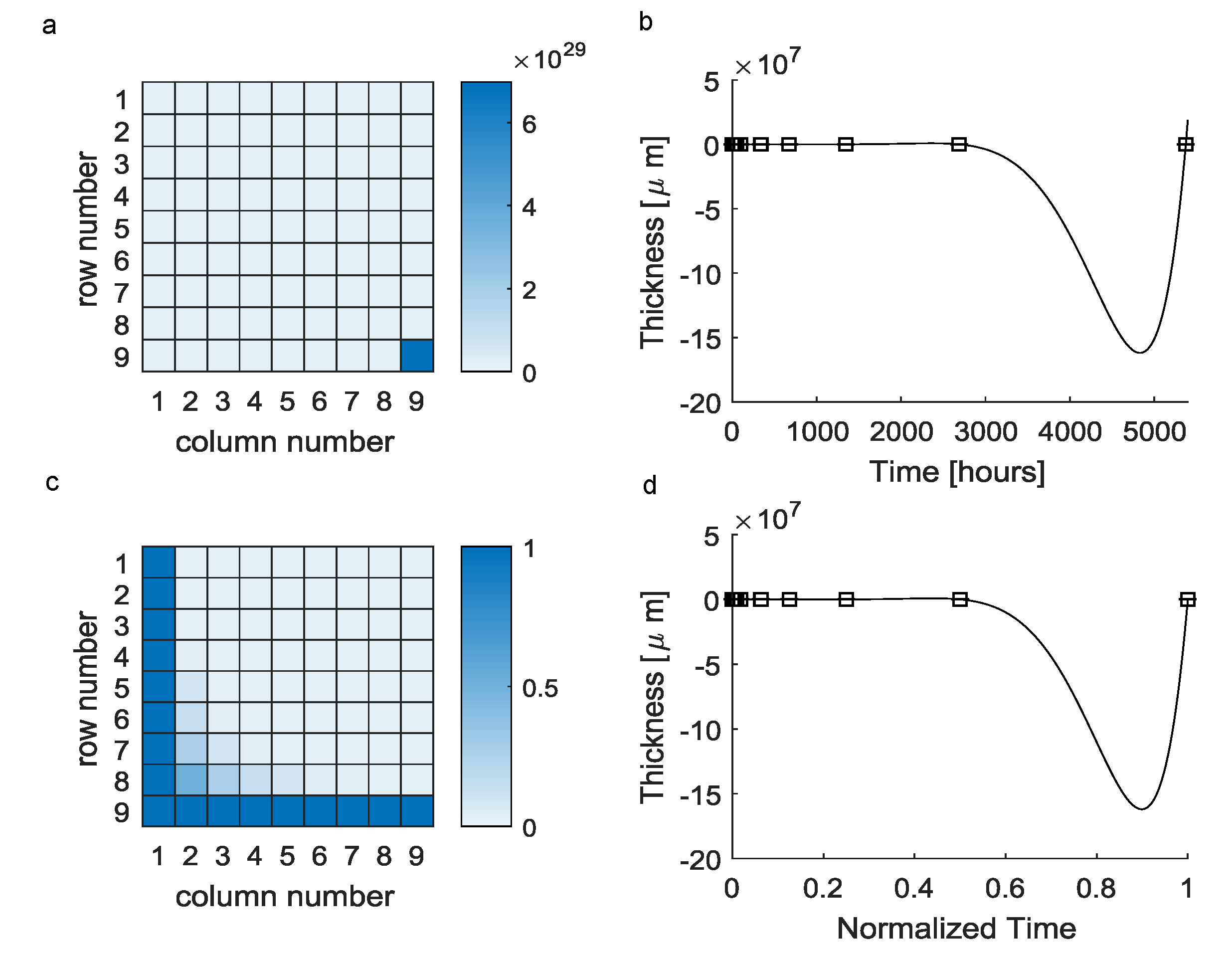
Figure 1. Vandermonde-based interpolation (black squares = mean experimental values, solid lines = theoretical predictions): (a) The huge difference among the element 9,9 and the other ones resulted in an ill-conditioned matrix. (b) The interpolating polynomial function was affected by the Runge phenomenon, resulting in nonphysical predictions for inter-interval values (negative values). (c) The normalization of times over the maximum experimental time lead to a better conditioned matrix. (d) Moreover, in the case of time normalization, the performances of the interpolating polynomials were unchanged.
Applsci 11 08568 g001
Figure 2. Interpolation through standard Lagrange polynomials: (a) Standard Lagrange polynomials (solid lines) were able to fit all the experimental data points (black squares). In this case, the function was the same as the function in Figure 1a, which was obtained through the Vandermonde-based interpolation. As a consequence, the numerical problems affecting the prediction of the thickness over time were the same. (b) Lagrange polynomials fitting all experimental points together with an extrapolated supplementary point. This function was still affected by the Runge phenomenon, but the magnitude of differences between predictions and experimental values was lower (i.e., about 1 × 10 7 ). (c) Lagrange polynomials fitting all experimental points together with two extrapolated supplementary points. Numerical errors still affected the interpolating function leading to nonphysical predictions, even if the magnitude of errors was lowered to about 1 × 10 6 . (d) Lagrange polynomials fitting all experimental points together with three extrapolated supplementary points. The Runge phenomenon still affected the interpolating polynomial function, which again resulted in nonphysical predictions. The magnitude of errors was further lowered to about 1 × 10 5 .
Applsci 11 08568 g002
Figure 3. Values of the H m , i numerical coefficients in Equation (10). For each candidate function all the values of each H m vector are reported in lines. These values are the numerical coefficients needed to provide the linear combination of J H S i ( t ) functions to express each w m ( t ) function.
Applsci 11 08568 g003
Figure 4. Reproduction of experimental data through the novel w n ( t ) functions (black squares = mean values, error bars = ± standard deviation, solid lines = theoretical predictions, dotted lines = 90 % confidence prediction bounds). (a) The function w 0 ( t ) (m = 0) was unable to reproduce experimental values since it assumed a constant value. (b) The function w 1 ( t ) (m = 1) was able to reproduce experiments with R 2 = 0.8661 . (c) The function w 2 ( t ) (m = 2) was able to reproduce experiments with R 2 = 0.9195 . (d) The function w 3 ( t ) (m = 3) reproduced experiments with R 2 = 0.9197 . (e) The function w 4 ( t ) (m = 4) reproduced experiments with R 2 = 0.9221 . (f) The function w 5 ( t ) (m = 5) reproduced experimental data with R 2 = 0.9190 .
Applsci 11 08568 g004
Figure 5. (a) The natural logarithm of the Λ f index was used to account for the intensity of the Runge phenomenon since it is able to graphically show whether approximating functions were affected by the Runge phenomenon. The first approximation obtained through the Vandermonde approach resulted in a positive value of l n ( Λ g 9 ( t ) ) . Similarly, for g 9 ( t ) , , g 12 ( t ) , this logarithm was positive since the Runge phenomenon affected predictions. On the contrary, for w 1 ( t ) , , w 5 ( t ) , this logarithm resulted in negative values and the Runge phenomenon did not affect numerical predictions of inter-interval values. For the function w 0 ( t ) , the index l n ( Λ w 0 ( t ) ) increased without bound towards (not shown within the plot). (b) Overall suitability: Considering both the ability of each candidate function to reproduce experimental values and the intensity of the Runge phenomenon affecting numerical predictions, the overall suitability shows that only the w n ( t ) family was able to reproduce experiments in a suitable way. Among the w n ( t ) functions, the w 4 ( t ) was also the most suitable to reproduce experimental data for inter-interval times.
Applsci 11 08568 g005
Table 1. Elements of the a vector, fully characterizing the candidate function resulting from the classic Vandermonde approach.
Elements of the a VectorValue
a 0 0
a 1 −0.276
a 2 +0.015
a 3 1.640 × 10 4
a 4 + 6.339 × 10 7
a 5 1.019 × 10 9
a 6 + 7.121 × 10 13
a 7 2.057 × 10 16
a 8 + 1.947 × 10 20
Table 2. The elements of the x vector, fully characterizing the interpolating Lagrange polynomials. The numeric values of the x vector elements for the functions g 10 ( t ) , g 11 ( t ) , g 12 ( t ) are shown in columns 1, 2, 3, respectively.
ElementsTotal Time Points n tot = 9 + 1Total Time Points n tot = 9 + 2Total Time Points n tot = 9 + 3
x 0 000
x 1 0.278 0.280 0.282
x 2 + 0.015 + 0.015 + 0.015
x 3 1.687 × 10 04 1.687 × 10 04 1.764 × 10 04
x 4 + 6.776 × 10 07 + 7.162 × 10 07 + 7.532 × 10 07
x 5 1.182 × 10 09 1.331 × 10 09 1.478 × 10 09
x 6 + 9.692 × 10 13 + 1.225 × 10 12 + 1.494 × 10 12
x 7 3.840 × 10 16 5.922 × 10 16 8.382 × 10 16
x 8 + 7.081 × 10 20 + 1.530 × 10 19 + 2.714 × 10 19
x 9 4.850 × 10 24 1.998 × 10 23 5.051 × 10 23
x 10 + 1.035 × 10 24 + 5.016 × 10 27
x 11 2.060 × 10 31
Publisher’s Note: MDPI stays neutral with regard to jurisdictional claims in published maps and institutional affiliations.