Mathematical Determination of the Upper and Lower Limits of the Diffuse Fraction at Any Site

Abstract

A mathematical method for accurately determining the upper and lower diffuse-fraction (k_d) limits that divide the sky into clear, intermediate, and overcast is developed. Fourteen sites around the world are selected for demonstrating the methodology. The upper and lower k_d values for these sites are determined from scatter plots of direct-normal solar radiation vs. k_d pairs over the typical meteorological year of each site. They vary between 0.73 and 0.80 for the upper and between 0.24 and 0.27 for the lower k_d limits. Plots of sunshine duration (SSD) vs. k_d are prepared for 12 of the 14 sites. These plots show a decreasing trend in SSD with increasing values of k_d, as anticipated. According to local climatology, the number of the SSD values in each sky-condition classification varies from site-to-site.

1. Introduction

The estimation of solar radiation on the surface of the Earth on either horizontal or tilted planes has long been recognised an important parameter in a variety of fields such as atmospheric environment, e.g., [1], terrestrial ecosystems, e.g., [2], terrestrial climate, e.g., [3], and solar energy applications, e.g., [4]. Because of the scarcity of solar radiation platforms that may provide measurements of the total (or global) solar radiation to the above applications, solar models started appearing in the international literature as early as in 1950′s. The total solar radiation is the sum of two components: the diffuse solar radiation and the direct (or beam) one. The latter can accurately be estimated via explicit atmospheric transmission relationships. It is, therefore, the diffuse component that must be simulated satisfactorily; however, this solar component is very difficult to accurately be estimated due to numerous scattering processes of the solar rays that take place in the atmosphere under a clear sky and moreover in the presence of clouds on a cloudy day. This fact has triggered a lot of research for the development of various models that pursue to estimate as accurately as possible the diffuse solar component. Such models are numerous in the international literature, e.g., [5,6,7]. Most of them use the diffuse fraction (k_d), which is the ratio of diffuse-to-global solar radiation as function of other parameter (or parameters) that can easily be calculated, be measured or are known; such parameters are the clearness index (k_t), which is the ratio of the global-to-the-extraterrestrial solar radiation, or the geographical latitude (φ), e.g., [8]. Even though k_t or k_d can be computed in one way or another, it is very important for solar energy engineers to know their upper and lower limits that divide the sky conditions into clear, intermediate and overcast. Several such limits have been provided by many researchers. All of them are based on solar measurements or solar modelling, e.g., [9,10]. This is, therefore, the reason that these limits are considered empirical as they are not based on a standard methodology.

The above gap is bridged in the present study. In other words, this work develops a mathematical methodology for determining the upper and lower limits of k_d. The methodology proves to be universal, but the values of the upper and lower k_d limits are site-dependent. Such a work is presented for the first time in the international literature.

2. Materials and Methods

This Section gives a full account of the new (mathematical) method that accurately determines the upper and lower limits of k_d at a site.

To apply the methodology, a typical meteorological year (TMY) must preferably be used instead of a long period of measurements or model simulations. This peculiarity is based on the fact that a TMY refers to all representative situations of the included parameters that occur within a year, while a long-term series of measurements or model simulations contains extreme values of the included parameters; the second, therefore, option may result in a broader dispersion of the calculated k_d values. On the other hand, TMYs are nowadays used more often in many climatological studies, e.g., [11,12,13].

The selected solar radiation parameter to vary with k_d is the direct horizontal solar radiation (H_b) because of much less dispersion of the H_b-k_d paired values in comparison with the cases of the functions H_g (global horizontal solar radiation) vs. k_d or H_d (diffuse horizontal solar radiation) vs. k_d. Even in the case of the direct horizontal solar radiation, the scatter plot of H_b vs. k_d is found to be greater than that of the relationship H_bn (direct-normal solar radiation) vs. k_d. Figure 1 shows this difference; here hourly mean H_b, H_bn and k_d values have been plotted for the typical month of January of the TMY-BOU (Boulder, USA) derived from the PV-GIS platform [14,15] (see below for description). Therefore, the H_bn solar component is considered in the rest of the analysis.

The mathematical determination of the upper and lower limits of k_d in a diagram as that of Figure 1b is fully described here. The first step is to find the best-fit curve to the H_bn-k_d data points. A second-order polynomial of the form H_bn = a k_d² + b k_d + c was used, where a, b, c are the polynomial coefficients. This type of best-fit curve was selected as the results obtained showed that it is sufficient. Figure 2 shows the best-fit black curve to the scatter plot of Figure 1b, which has the expression H_bn = 902.30 k_d² − 2087.44 k_d + 1188.58, R² = 0.996. As WMO recommends that the sunshine duration is measured when H_bn > 120 Wm⁻², the green line represents this threshold. This straight line crosses the best-fit curve at a certain point (k_du,H_bnWMO = 120). Since the y-axis value is known (120 Wm⁻²), solving the above second-order equation for k_d, two roots are obtained and the lower-than-1 is considered because k_d cannot go higher than 1 by definition; in this case, the accepted solution is k_du = 0.76.

The next step is to find the equation of the straight line that is tangent to the best-fit curve at the point C (0.76,120); this point is the crossing point between the best-fit curve and the WMO-defined threshold for SSD measurements. This line expresses the first derivative of the best-fit curve at the point C; in other words, it represents the slope of the best-fit line at C. This is done by taking the first derivative of the H_bn expression (H′_bn) in respect to k_d and replacing k_d with 0.76. It is found that H′_bn = −715.94 Wm⁻². Then, H_bn − 120 = −715.94 (k_d − 0.76) from which the expression for the tangent line is H_bn = −715.94 k_d + 664.12. This straight line is the BC in Figure 2. A rectangle triangle ABC is then formed.

The third step is to draw the two medians from the vertexes A and B of the triangle ABC to their opposite sides, i.e., the lines AD and BE, respectively. The two lines are crossed at M; if a straight line parallel to the y-axis is drawn through M, i.e., the blue line MG, this crosses the x-axis at a value, which is the lower limit of k_d. From the Euclidian geometry, it is known that AG = AC/3. This means that if the upper k_d value at the point C is obtained (k_du), then very easily the lower k_d value at the point G (k_dl) can be calculated: k_dl = k_du/3. This way, the estimated k_du and k_dl values divide the sky conditions in clear skies, intermediate skies, and overcast skies at a site as shown in Figure 2.

The above methodology was applied to 14 sites around the world. The selection has been based on the following criteria: (i) different environmental characteristics, (ii) spread across the continents, and (iii) availability of TMY.

Table 1. Selected sites for the application of the mathematical determination of the k_du and k_dl limits. φ and λ are the geographical latitudes and longitudes of the sites, respectively; φ is given in the northern (N) or the southern (S) hemisphere, and λ east (E) or west (W) of the Greenwich meridian. The values of both φ and λ have been rounded to the second decimal digit. In column 9, I denotes rural and II denotes urban environment. The period of measurements is given in the last column. The selection of the sites and their solar radiation data were based on the BSRN (Baseline Surface Radiation Network), except for Athens (ATH); in this case, data from the Actinometric Station of the National Observatory of Athens not belonging to BSRN were used. The abbreviations of the sites (except for Athens) are those provided by the BSRN typology. Description of the BSRN operation is found in [16].

#	Site (Abbreviation)	Location	φ (deg)	λ (deg)	z (m asl)	Surface Type	Topography	I/II	Period
1	Athens (ATH)	Greece	37.97 N	23.72 E	107	shrubs, trees	hilly	II	1953–present
2	Boulder (BOU)	USA	40.05 N	105.01 W	1577	grass	flat	I	1992–2016
3	Carpentras (CAR)	France	44.08 N	5.06 E	100	cultivated	hilly	I	1996–2018
4	De Aar (DAA)	South Africa	30.67 S	23.99 E	1287	sand	flat	I	2000–present
5	Gandhinagar (GAN)	India	23.11 N	72.63 E	65	shrubs	flat	II	2014–present
6	Huancayo Observatory (OHY)	Peru	12.05 S	75.32 W	3314	grass	mountain valley	I	2017–present
7	Ilorin (ILO)	Nigeria	8.53 N	4.57 E	350	shrubs	flat	I	1992–2005
8	Kishinev (KIS)	Moldova	47.00 N	28.82 E	205	grass	flat	II
9	Lerwick (LER)	UK	60.14 N	1.18 W	80	grass	hilly	I	2001–present
10	Lindenberg (LIN)	Germany	52.21 N	14.12 E	125	cultivated	hilly	I	1994–present
11	Payerne (PAY)	Switzerland	46.82 N	6.94 E	491	cultivated	hilly	I	1992–present
12	Regina (REG)	Canada	50.21 N	104.71 W	578	cultivated	flat	I	1995–2011
13	Sonnblick (SON)	Austria	47.05 N	12.96 E	3109	rocks	mountain top	I	2013–present
14	Solar Village (SOV)	Saudi Arabia	24.91 N	46.41 E	650	desert, sand	flat	I	1998–2002

deploys the selected sites in alphabetical order together with their geographical coordinates and environmental description. Sites that do not meet criterion (iii) may not be appropriate for applying this methodology. Figure 3 gives the distribution of the 14 sites over the world.

For the sake of the present analysis, TMYs for the selected sites have been downloaded from the PV-GIS platform [17,18]. These typical meteorological years have been derived from a combination of satellite and re-analysis data in the period 2005–2014. Each TMY contains the following parameters: date, time (h UTC), dry-bulb temperature (in degC), relative humidity (in %), global horizontal solar irradiance (H_g, in Wm⁻²), direct-normal solar irradiance (H_bn, in Wm⁻²), diffuse horizontal solar irradiance (H_d, in Wm⁻²), infra-red horizontal solar irradiance (in Wm⁻²), wind speed (in ms⁻¹), wind direction (in deg), barometric pressure (P_z, in Pa) at the site’s altitude (z, in m), and a control parameter. The meteorological and solar radiation values are hourly averages. Therefore, from the 14 downloaded TMYs new files were created to contain the necessary parameters: date, time (h UTC), H_g, H_bn, and H_d. Conversion of time from UTC (universal time constant) into LST (local standard time) at each site was applied to all files. Then, an own-developed routine, named XRONOS.bas in Basic programming language (xronos means time in Greek with x being spelled as ch), was used to derive the solar altitude (γ, in deg) at 30 minutes past the hour LST. For example, the value of any parameter in the data base at 10.00 LST denotes its average value between 09.01 LST and 10.00 LST. The XRONOS.bas algorithm calculated γ at 09.30 LST and this value was assigned to all parameters at 10.00 LST. Finally, the hourly values of k_d were computed from concurrent values of H_g and H_d, i.e., k_d = H_d/H_g. In cases that H_d and/or H_g contained zero values, no value was assigned to k_d. Correspondingly, no value was assigned to H_bn, too. In plotting the (x, y) data pairs, i.e., (k_d, H_bn), the hourly values of these two parameters were considered for all γ > 5 deg. This way, 14 plots of H_bn-k_d were derived to apply the methodology and derive the individual k_dl and k_du limits for the sites. The plots are deployed and discussed in Section 3.1.

3. Results

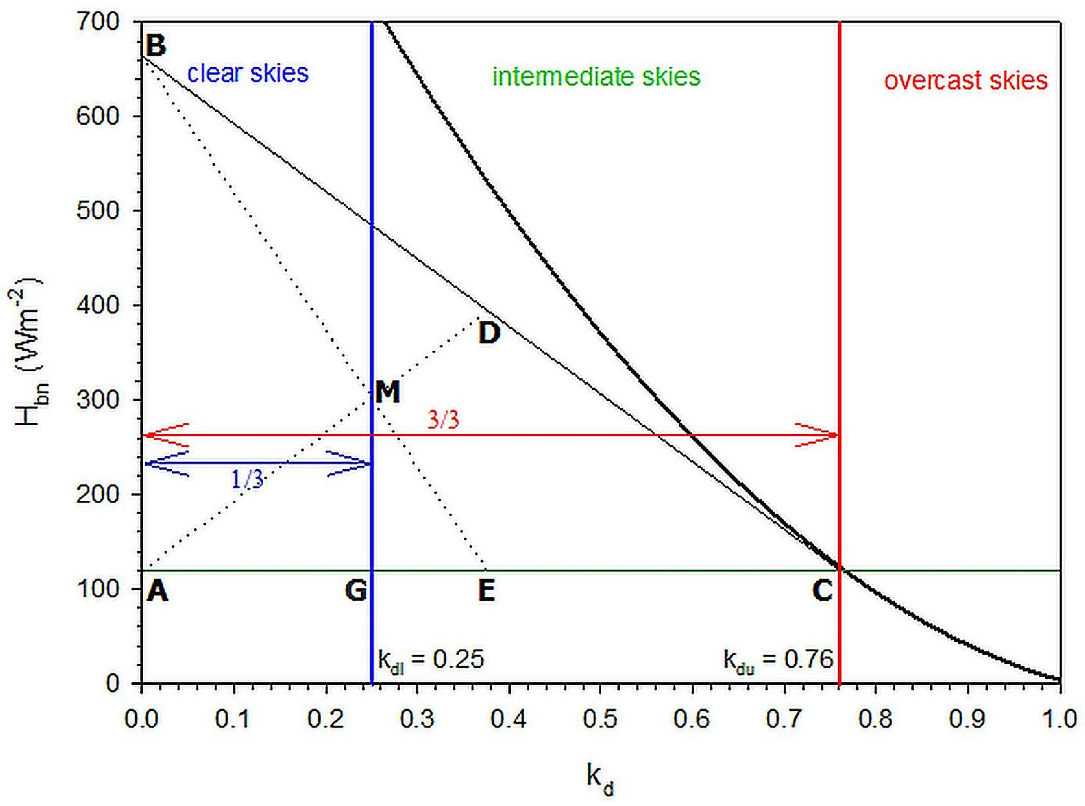
3.1. Determination of the k_d Limits

This section presents the results from the application of the developed methodology to the 14 sites. Figure 4, Figure 5, Figure 6, Figure 7, Figure 8, Figure 9 and Figure 10 show the graphical estimation of the k_du and k_dl values for all 14 sites. The H_bn-k_d values refer to the PV-GIS TMYs of the 14 sites.

From the above Figures it is seen that different spreads in the scatter plots exist. This variance is least at the ATH, GAN, KIS, LIN, REG, and SOV sites and greatest at the BOU, LER, and POY ones. The broader variance in the H_bn-k_d data pairs is possibly due to the changing weather conditions at these sites (fast moving clouds, prevailing heavy/light cloudiness most of the time), which affect the H_d values in the estimation of k_d. On the other hand, missing solar radiation values occur in the case of the OHY site; this results in fewer data points than at the rest of the sites.

Table 2. Second-order polynomial expression for the function H_bn vs. k_d with R², k_du, and k_dl values. All values have been rounded to the second decimal digit. The year in parenthesis in column 1 denotes the period of the downloaded solar radiation measurements from the BSRN sites. The criterion for the year selection was to be outside the PV-GIS TMY period of 2004–2015, if possible.

Site (Year)	Equation of the Best-Fit Curve	R2	kdu	kdl
AΤH (2000)	Hbn = 750.35 kd2 − 1911.13 kd + 1160.42	0.99	0.79	0.26
BOU (1999)	Hbn = 764.84 kd2 − 1906.61 kd + 1145.82	0.99	0.79	0.26
CAR (2018)	Hbn = 868.13 kd2 − 2035.91 kd + 1172.93	0.99	0.77	0.26
DAA (2017)	Hbn = 829.67 kd2 − 2009.26 kd + 1182.98	0.99	0.78	0.26
GAN (2015)	Hbn = 923.82 kd2 − 2150.63 kd + 1230.29	≈1.00	0.77	0.26
OHY (2018)	Hbn = 715.87 kd2 − 1879.32 kd + 1165.29	0.99	0.80	0.27
ILO (1999)	Hbn = 796.31 kd2 − 2007.88 kd + 1208.37	0.99	0.79	0.26
KIS (2020)	Hbn = 781.01 kd2 − 1935.32 kd + 1155.12	≈1.00	0.78	0.26
LER (2003)	Hbn = 930.30 kd2 − 2020.92 kd + 1097.60	0.94	0.73	0.24
LIN (2018)	Hbn = 779.37 kd2 − 1929.96 kd + 1151.03	0.99	0.78	0.26
PAY (2013)	Hbn = 715.85 kd2 − 1856.32 kd + 1140.65	0.99	0.79	0.26
REG (2003)	Hbn = 779.37 kd2 − 1929.96 kd + 1151.03	≈1.00	0.78	0.26
SOV (2002)	Hbn = 919.21 kd2 − 2192.18 kd + 1270.02	0.99	0.78	0.26
SON (2018)	Hbn = 704.02 kd2 − 1833.67 kd + 1129.45	0.99	0.79	0.26

gives the expressions of the best-fit curves, their R² that determine the variance, and the estimation of the k_du and k_dl values. Since these values are similar for all sites examined, one could adopt universal values that are the average of the distinct ones; in this case a universal k_du would be 0.78 and a universal k_dl 0.26. Nevertheless, these averages are only indicative, because they refer to a small number of sites over the globe.

3.2. Evaluation of the Methodology

To show the applicability of the method developed in Section 2, Figure 11, Figure 12, Figure 13, Figure 14, Figure 15, Figure 16 and Figure 17 show the distribution of the (k_d,SSD) pairs during the years shown in parentheses in column 1, Table 2. The SSD values were derived from the BSRN data, meeting the H_bn > 120 Wm⁻² WMO criterion; moreover, the SSD values from the ATH station are real 1-min measurements with the aid of an EKO MS-90 direct-normal-irradiance sensor. All (k_d,SSD) data values are hourly ones in the corresponding year of the site (column 1, Table 2). Therefore, SSDs for k_du < k_d ≤ 1 correspond to overcast-, for k_dl < k_d ≤ k_du to intermediate-, and for 0 ≤ k_d ≤ k_dl to clear-sky conditions.

The shape of the scattered data points in the above diagrams is the expected one, i.e., decreasing SSD values with increasing k_d. Nevertheless, this self-evident pattern is not repeated at the GAN and ILO sites; this may be due to the solar radiation data quality, which, in the case of ILO, may be unacceptable. Therefore, these two sites are excluded from further analysis. Moreover, the site of OHY presents some low SSD values for clear skies (i.e., for 0 ≤ k_d ≤ 0.26), but the number of such values is small, and, therefore, this site is included in the analysis that follows.

In each of the remaining 14 sites, the number of the (k_d,SSD) hourly pairs is maximum (8760 or 8784 for a non-leap or a leap year, respectively); these numbers include night-time values, which were not taken into account. The analysis that follows concerns the number of daytime hourly pairs that represent the three sky condition statuses (overcast, intermediate, clear).

Table 3. Number of (daytime) hourly SSD values at each site within the year indicated for the various k_d conditions; percentages of the individual cases to the total are given in parentheses.

Site (Year)	kdu < kd ≤ 1 Overcast Skies	kdl < kd ≤ kdu Intermediate Skies	0 ≤ kd ≤ kdl Clear Skies	0 ≤ kd ≤ 1 All Skies
AΤH (2000)	919 (20.9%)	1879 (42.7%)	1602 (36.4%)	4400 (100%)
BOU (1999)	1477 (31.7%)	1429 (30.6%)	1758 (37.7%)	4664 (100%)
CAR (2018)	1799 (37.1%)	1556 (32.1%)	1496 (30.8%)	4851 (100%)
DAA (2017)	733 (15.5%)	1288 (27.1%)	2715 (57.4%)	4736 (100%)
GAN (2015)	-	-	-	-
OHY (2018)	908 (24.3%)	957 (25.5%)	1881 (50.2%)	3746 (100%)
ILO (1999)	-	-	-	-
KIS (2020)	1524 (36.2%)	1525 (36.2%)	1161 (27.6%)	4210 (100%)
LER (2003)	3476 (68.8%)	1225 (24.2%)	354 (7.0%)	5055 (100%)
LIN (2018)	1652 (41.5%)	1515 (38.1%)	811 (20.4%)	3978 (100%)
PAY (2013)	2100 (43.5%)	1743 (36.1%)	986 (20.4%)	4829 (100%)
REG (2003)	2049 (37.6%)	1932 (35.5%)	1467 (26.9%)	5448 (100%)
SOV (2002)	872 (18.3%)	2199 (46.0%)	1704 (35.7%)	4775 (100%)
SON (2018)	2624 (60.2%)	952 (21.8%)	781 (18.0%)	4357 (100%)

shows the results.

The differentiation in the total daytime values (column 5, Table 3) is due to the geographical location of the sites, which dictates the daylight pattern, i.e., the daylength. On the other hand, the variation in the SSD values under the three sky conditions is much influenced by the prevailing climatology at each site.

4. Conclusions and Discussion

A mathematical formulation for the determination of the upper and lower diffuse-fraction limits was developed for the first time worldwide. The methodology was based on existing or prepared TMY for the site into consideration. Such a TMY can be downloaded free-of-charge from the PV-GIS website. The TMY must include hourly values of the global horizontal, diffuse horizontal, and direct-normal solar irradiances. Hourly values of the diffuse fraction can then be derived.

The method consists of the following analytical steps.

Step 1. Prepare a scatter plot of the hourly direct-normal solar radiation vs. diffuse-fraction values that are included in the TMY for the site into consideration.

Step 2. Estimate the best-fit second-order polynomial to the data points of step 1.

Step 3. Find the upper diffuse-fraction limit, k_du, at the intersection between the line y = 120 Wm⁻² and the best-fit curve, i.e., point C (k_du,120).

Step 4. Find the equation of the straight line, which is tangent to point C.

Step 5. Find point B where the straight line of step 4 crosses the y axis.

Step 6. Observe the orthogonal triangle formed by the vertexes A (0,0), B, C (k_du,120).

Step 7. Draw the medians from the vertexes A and B, crossing each other at M.

Step 8. Draw a straight line from M normal to AC, crossing AC at G.

Step 9. Find the lower diffuse-fraction limit, k_dl, on the x axis, or estimate it as k_dl = k_du/3.

Fourteen sites were selected worldwide under the criteria of (i) existing TMY at the PV-GIS platform, and (ii) spread of the locations across the continents. The above procedure was applied to the 14 sites and their k_du, k_dl values were calculated.

To evaluate the methodology derived, 1-min solar radiation data were downloaded from BSRN for 11 sites and for 1 year for each location. Data for the ATH, KIS, and LIN sites were provided free-of-charge. Hourly values of (k_d, SSD) pairs were estimated and statistics about the number of SSD under clear (0 ≤ k_d ≤ k_dl), intermediate (k_dl < k_d ≤ k_du), and overcast (k_du < k_d ≤ 1) skies were prepared. The analysis showed that, in most sites (GAN and ILO were not taken into account), the anticipated decreasing trend of SSD with increasing values of k_d was confirmed. Moreover, the number of the SSD values varied from site-to-site according to local climate and sky-conditions considered. The analysis showed that the k_dl and k_du values ranged between 0.24 and 0.26, and between 0.73 and 0.80, respectively, as average values over the selected sites.

The value of the presented methodology lies not only in the accurate determination of the k_du and k_dl values at any site, but also contributes to the solar radiation climatology of a site, and the derivation of its SSD values, if they are not available. The estimation of the SSD values is not, of course, that accurate because of the great dispersion of the SSD-k_d pairs (Figure 11, Figure 12, Figure 13, Figure 14, Figure 15, Figure 16 and Figure 17). Nevertheless, the methodology gives a qualitative indication; this is something than nothing.

It must be mentioned here that various attempts to estimate k_d in the past were based on modelling than measurements as in the present study. The use of models may result in reduced accuracy because the intrinsic error in the estimation of k_d increases in comparison with a measurements-based methodology. For instance, Dervishi and Mahdavi [9] used 8 models for the estimation of k_d as function of k_t; all of them gave high MBD (mean bias difference, in %) and RMSD (root mean square difference, in %) values. Last but not least, the present study provided a methodology to compute the two k_d limits from which one may categorise the sky at his/her site in the three main statuses: clear, intermediate, and overcast. This was done for the first-time worldwide.

The developed mathematical formulation, therefore, clearly determines the upper and lower diffuse-fraction limits, and seems to work quite efficiently over the globe. Therefore, it may have a universal character. However, the method should be tested for applicability at sites in Russia, central and south Asia, Japan, Australia, and Oceania in order to fully manifest its universality.

References

1. Giesen, R.H.; van den Broeke, M.R.; Oerlemans, J.; Andreassen, L.M. Surface Energy Balance in the Ablation Zone of Midtdalsbreen, a Glacier in Southern Norway: Interannual Variability and the Effect of Clouds. J. Geophys. Res. 2008, 113, D21111. [Google Scholar] [CrossRef]
2. Steinbacher, M.; Bingemer, H.G.; Schmidt, U. Measurements of the Exchange of Carbonyl Sulfide (OCS) and Carbon Disulfide (CS 2) between Soil and Atmosphere in a Spruce Forest in Central Germany. Atmos. Environ. 2004, 38, 6043–6052. [Google Scholar] [CrossRef]
3. Bojinski, S.; Verstraete, M.; Peterson, T.C.; Richter, C.; Simmons, A.; Zemp, M. The Concept of Essential Climate Variables in Support of Climate Research, Applications, and Policy. Bull. Am. Meteorol. Soc. 2014, 95, 1431–1443. [Google Scholar] [CrossRef]
4. Kambezidis, H.D. Current Trends in Solar Radiation Modeling: The Paradigm of MRM. J. Fundam. Renew. Energy Appl. 2016, 6, 2014–2015. [Google Scholar] [CrossRef]
5. Babatunde, A.; Vincent, O.O. Estimation of Hourly Clearness Index and Diffuse Fraction Over Coastal and Sahel Regions of Nigeria Using NCEP/NCAR Satellite Data. J. Energy Res. Rev. 2021, 7, 1–18. [Google Scholar] [CrossRef]
6. Badescu, V.; Gueymard, C.A.; Cheval, S.; Oprea, C.; Baciu, M.; Dumitrescu, A.; Iacobescu, F.; Milos, I.; Rada, C. Computing Global and Diffuse Solar Hourly Irradiation on Clear Sky. Review and Testing of 54 Models. Renew. Sustain. Energy Rev. 2012, 16, 1636–1656. [Google Scholar] [CrossRef]
7. El-Sebaii, A.A.; Al-Hazmi, F.S.; Al-Ghamdi, A.A.; Yaghmour, S.J. Global, Direct and Diffuse Solar Radiation on Horizontal and Tilted Surfaces in Jeddah, Saudi Arabia. Appl. Energy 2010, 87, 568–576. [Google Scholar] [CrossRef]
8. Berrizbeitia, S.E.; Gago, E.J.; Muneer, T. Empirical Models for the Estimation of Solar Sky-Diffuse Radiation. A Review and Experimental Analysis. Energies 2020, 13, 701. [Google Scholar] [CrossRef] [Green Version]
9. Dervishi, S.; Mahdavi, A. Computing Diffuse Fraction of Global Horizontal Solar Radiation: A Model Comparison. Sol. Energy 2012, 86, 1796–1802. [Google Scholar] [CrossRef] [PubMed] [Green Version]
10. Hijazin, M.I. The Diffuse Fraction of Hourly Solar Radiation for Amman/Jordan. Renew. Energy 1998, 13, 249–253. [Google Scholar] [CrossRef]
11. Grudzińska, M.; Jakusik, E. The Efficiency of a Typical Meteorological Year and Actual Climatic Data in the Analysis of Energy Demand in Buildings. Build. Serv. Eng. Res. Technol. 2015, 36, 658–669. [Google Scholar] [CrossRef]
12. Chan, A.L.S. Generation of Typical Meteorological Years Using Genetic Algorithm for Different Energy Systems. Renew. Energy 2016, 90, 1–13. [Google Scholar] [CrossRef]
13. Fernández, M.D.; López, J.C.; Baeza, E.; Céspedes, A.; Meca, D.E.; Bailey, B. Generation and Evaluation of Typical Meteorological Year Datasets for Greenhouse and External Conditions on the Mediterranean Coast. Int. J. Biometeorol. 2015, 59, 1067–1081. [Google Scholar] [CrossRef] [PubMed]
14. Müller, R.; Pfeifroth, U.; Träger-Chatterjee, C.; Trentmann, J.; Cremer, R. Digging the METEOSAT Treasure-3 Decades of Solar Surface Radiation. Remote Sens. 2015, 7, 8067–8101. [Google Scholar] [CrossRef] [Green Version]
15. Huld, T.; Müller, R.; Gambardella, A. A New Solar Radiation Database for Estimating PV Performance in Europe and Africa. Sol. Energy 2012, 86, 1803–1815. [Google Scholar] [CrossRef]
16. Driemel, A.; Augustine, J.; Behrens, K.; Colle, S.; Cox, C.; Cuevas-Agulló, E.; Denn, F.M.; Duprat, T.; Fukuda, M.; Grobe, H.; et al. Baseline Surface Radiation Network (BSRN): Structure and Data Description (1992–2017). Earth Syst. Sci. Data 2018, 10, 1491–1501. [Google Scholar] [CrossRef] [Green Version]
17. Urraca, R.; Gracia-Amillo, A.M.; Koubli, E.; Huld, T.; Trentmann, J.; Riihelä, A.; Lindfors, A.V.; Palmer, D.; Gottschalg, R.; Antonanzas-Torres, F. Extensive Validation of CM SAF Surface Radiation Products over Europe. Remote Sens. Environ. 2017, 199, 171–186. [Google Scholar] [CrossRef] [PubMed] [Green Version]
18. Urraca, R.; Huld, T.; Gracia-Amillo, A.; Martinez-de-Pison, F.J.; Kaspar, F.; Sanz-Garcia, A. Evaluation of Global Horizontal Irradiance Estimates from ERA5 and COSMO-REA6 Reanalyses Using Ground and Satellite-Based Data. Sol. Energy 2018, 164, 339–354. [Google Scholar] [CrossRef]
Figure 1. Variation of (a) Hb and (b) Hbn as function of kd for January of the PV-GIS TMY-BOU. All data points are hourly values. Dispersion is greater in (a).
Applsci 11 08654 g001
Figure 2. Mathematical determination of the upper (kdu, red solid line) and lower (kdl, blue solid line) limits of kd that divide the skies into clear, intermediate, and overcast. The bold black solid line is the best-fit curve to the Hbn-kd data points that correspond to their hourly values; in this case the typical meteorological month of January, which belongs to the PV-GIS TMY-BOU, has been considered. The line BC is tangent to the best-fit line at C (0.76,120). M is the crossing point of the medians AD and BE. The MG line is normal to AC. From the Euclidian geometry AG = AC/3 in the rectangle triangle ABC; therefore, kdl = kdu/3 = 0.76/3 ≈ 0.25.
Applsci 11 08654 g002
Figure 3. Location of the 14 selected sites (green circles). The numbers in the circles correspond to the numbers in column 1 of Table 1.
Applsci 11 08654 g003
Figure 4. Determination of the kdu (red line) and kdl (blue line) values for the (a) ATH and (b) BOU sites.
Applsci 11 08654 g004
Figure 5. Determination of the kdu (red line) and kdl (blue line) values for the (a) CAR and (b) DAA sites.
Applsci 11 08654 g005
Figure 6. Determination of the kdu (red line) and kdl (blue line) values for the (a) GAN and (b) OHY sites.
Applsci 11 08654 g006
Figure 7. Determination of the kdu (red line) and kdl (blue line) values for the (a) ILO and (b) KIS sites.
Applsci 11 08654 g007
Figure 8. Determination of the kdu (red line) and kdl (blue line) values for the (a) LER and (b) LIN sites.
Applsci 11 08654 g008
Figure 9. Determination of the kdu (red line) and kdl (blue line) values for the (a) PAY and (b) REG sites.
Applsci 11 08654 g009
Figure 10. Determination of the kdu (red line) and kdl (blue line) values for the (a) SON and (b) SOV sites.
Applsci 11 08654 g010
Figure 11. Determination of clear, intermediate, and overcast skies for the (a) ATH and (b) BOU sites.
Applsci 11 08654 g011
Figure 12. Determination of clear, intermediate, and overcast skies for the (a) CAR and (b) DAA sites.
Applsci 11 08654 g012
Figure 13. Determination of clear, intermediate, and overcast skies for the (a) GAN and (b) OHY sites.
Applsci 11 08654 g013
Figure 14. Determination of clear, intermediate, and overcast skies for the (a) ILO and (b) KIS sites.
Applsci 11 08654 g014
Figure 15. Determination of clear, intermediate, and overcast skies for the (a) LER and (b) LIN sites.
Applsci 11 08654 g015
Figure 16. Determination of clear, intermediate, and overcast skies for the (a) PAY and (b) REG sites.
Applsci 11 08654 g016
Figure 17. Determination of the kdu (red line) and kdl (blue line) values for the (a) SON and (b) SOV sites.
Applsci 11 08654 g017