
Deep Reinforcement Learning-Based Network Routing Technology for Data Recovery in Exa-Scale Cloud Distributed Clustering Systems


Abstract
:1. Introduction
2. Background Principle
2.1. Principle of Erasure Coding
2.2. Principle of Deep Q-Network
3. Related Studies and Motivation
3.1. Studies Related to Erasure Coding
3.2. Supervised Learning-Based Network Routing
3.3. Reinforcement-Learning-Based Network Routing
3.4. Motivation
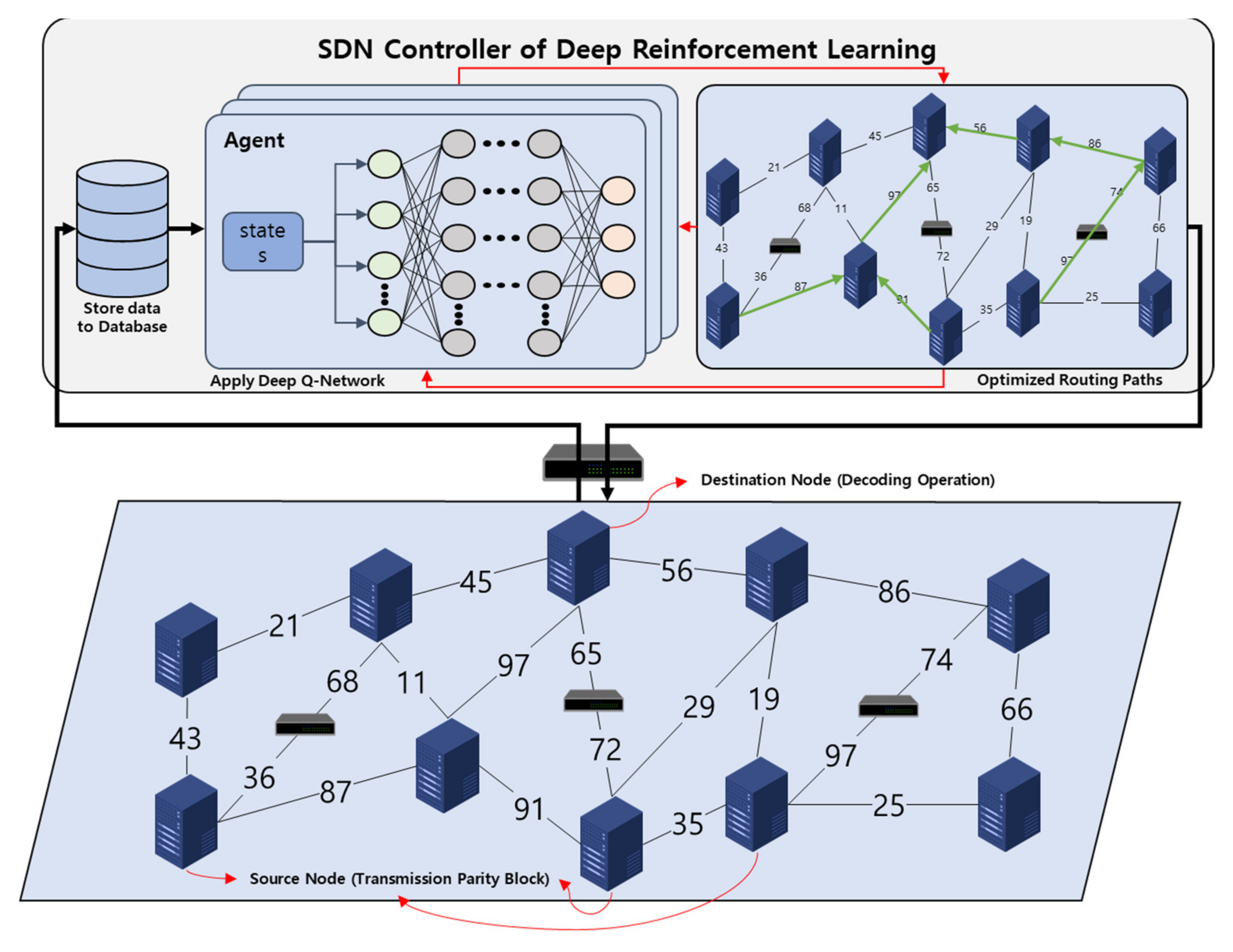
4. System Design
4.1. Overview
4.2. Database Storage
4.3. Performance of Deep Q-Network
4.4. Optimized Routing Paths
| Algorithm 1 DQN-based network routing in Erasure Coding network topology | |
| 1 | Input: hyper parameters of neural network, discount factor |
| 2 | Initialize experience replay memory |
| Initialize action-value function with random weights | |
| Initialize target action-value function with weights | |
| Initialize network route list | |
| Initialize complete network route 2d list | |
| 3 | For 1: do ( |
| 4 | For episodes = 1:100 do |
| 5 | With the probability select random action otherwise select = |
| Execution action , get reward and next state then update the network state | |
| 6 | Store the experience ( to |
| Sample random mini batch perform ( ) from in | |
| 7 | If episode terminates at step, then |
| Set target | |
| Else | |
| Set target | |
| End If | |
| Perform a gradient descent step on learning rate and with | |
| Every steps reset | |
| End For | |
| 8 | Append the last route path to list |
| List append to list | |
| 9 | Initialize all variable except ( |
| End For | |
| 10 | Output: Complete network route path from all source node to destination node |
5. Evaluation
5.1. Simulation Environment
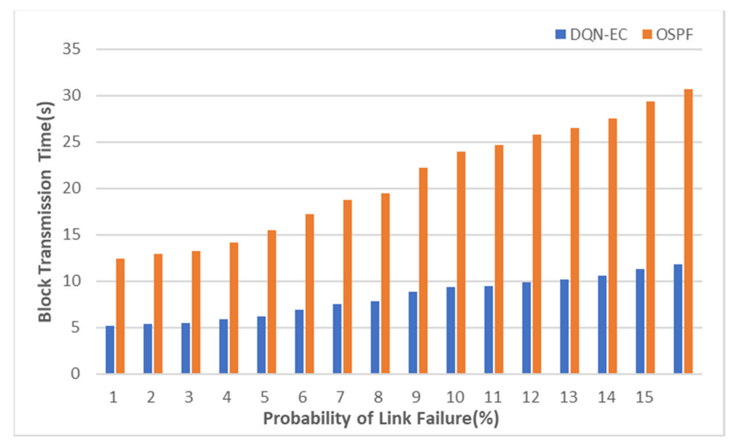
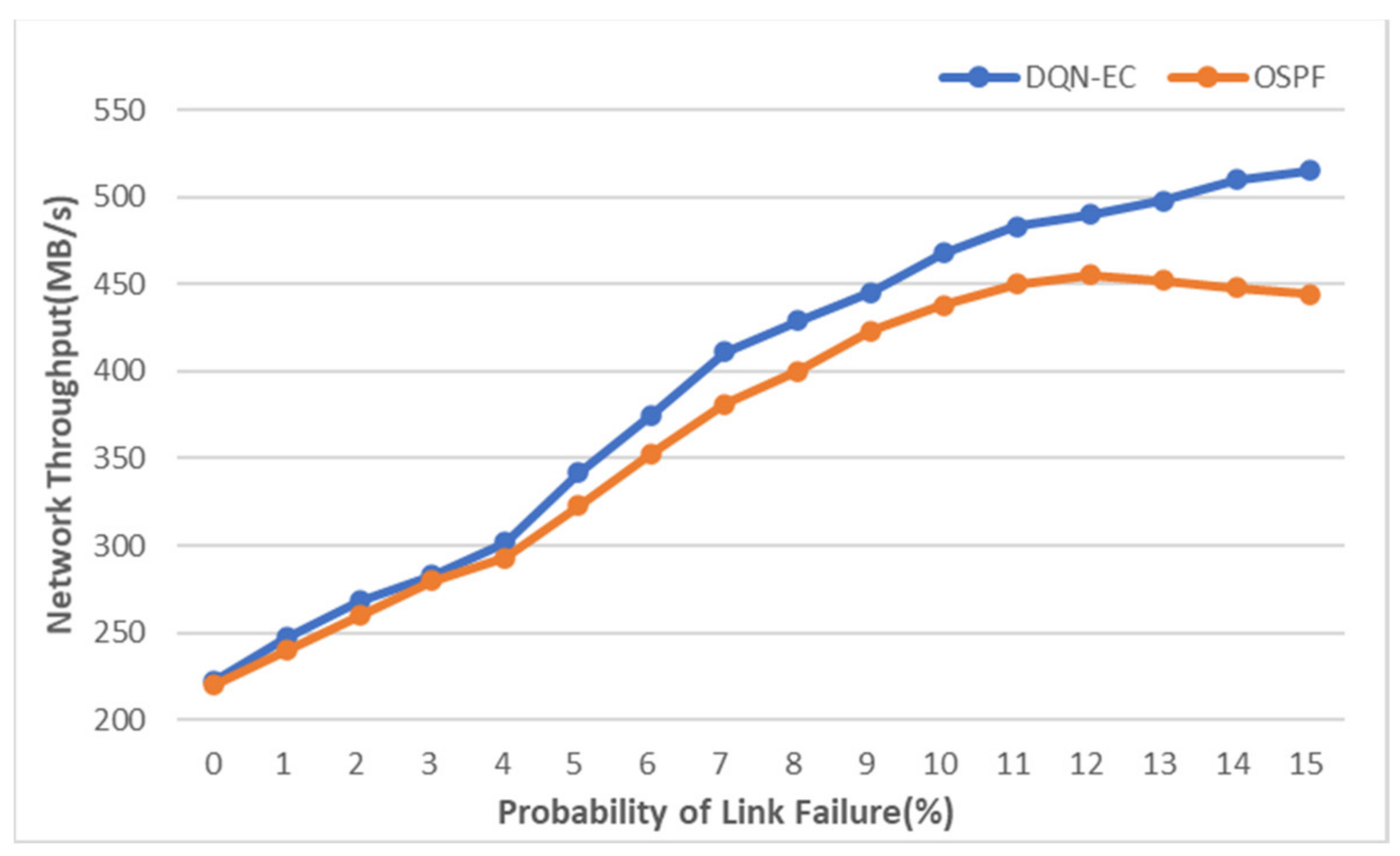
5.2. Evaluation Result of DQN-EC
5.3. Comparison and Summary of DQN-EC and Experiment Results
6. Conclusions
Author Contributions
Funding
Institutional Review Board Statement
Informed Consent Statement
Data Availability Statement
Conflicts of Interest
References
- Jiang, Y.; Liu, Q.; Dannah, W.; Jin, D.; Liu, X.; Sun, M. An Optimized Resource Scheduling Strategy for Hadoop Speculative Execution Based on Non-cooperative Game Schemes. Comput. Mater. Contin. 2020, 62, 713–729. [Google Scholar] [CrossRef]
- Astyrakakis, N.; Nikoloudakis, Y.; Kefaloukos, I.; Skianis, C.; Pallis, E.; Markakis, E.K. Cloud-Native Application Validation & Stress Testing through a Framework for Auto-Cluster Deployment. In Proceedings of the 24th International Workshop on Computer Aided Modeling and Design of Communication Links and Networks (CAMAD), Limassol, Cyprus, 11–13 September 2019; pp. 1–5. [Google Scholar] [CrossRef]
- Saadoon, M.; Hamid, S.H.A.; Sofian, H.; Altarturi, H.H.; Azizul, Z.H.; Nasuha, N. Fault tolerance in big data storage and processing systems: A review on challenges and solutions. ASEJ 2021, in press. [Google Scholar] [CrossRef]
- Shin, D.J. A Study on Efficient Store and Recovery Technology to Reduce the Disk Loading of Distributed File System in Big Data Environment. Master’s Thesis, Korea Polytechnic University, Siheung-si, Korea, 2020. [Google Scholar]
- Xia, J.; Guo, D.; Xie, J. Efficient in-network aggregation mechanism for data block repairing in data centers. Future Gener. Comput. Syst. 2020, 105, 33–43. [Google Scholar] [CrossRef]
- Wang, F.; Tang, Y.; Xie, Y.; Tang, X. XORInc: Optimizing data repair and update for erasure-coded systems with XOR-based in-network computation. In Proceedings of the 35th Symposium on Mass Storage Systems and Technologies (MSST), Santa Clara, CA, USA, 20–24 May 2019; pp. 244–256. [Google Scholar] [CrossRef]
- Kreutz, D.; Ramos, F.M.V.; Verissimo, P.E.; Rothenberg, C.E.; Azodolmolky, S.; Uhlig, S. Software-defined networking: A comprehensive survey. Proc. IEEE 2014, 103, 14–76. [Google Scholar] [CrossRef] [Green Version]
- Traffic Engineering (TE) Extensions to OSPF Version 2. Available online: https://www.hjp.at/doc/rfc/rfc3630.html (accessed on 5 June 2021).
- Pano-Azucena, A.D.; Tlelo-Cuautle, E.; Ovilla-Martinez, B.; Fraga, L.G.D.L.; Li, R. Pipeline FPGA-based Implementations of ANNs for the Prediction of up to 600-steps-ahead of Chaotic Time Series. J. Circuits Syst. Comput. 2021, 30, 2150164. [Google Scholar] [CrossRef]
- Shin, D.J.; Kim, J.J. Research on improving disk throughput in EC-based distributed file system. Psychol. Educ. 2021, 58, 9664–9671. [Google Scholar] [CrossRef]
- Plank, J.S. Erasure Codes for Storage Systems: A brief primer. Usenix Mag. 2013, 38, 44–50. [Google Scholar]
- Deng, M.; Liu, F.; Zhao, M.; Chen, Z.; Xiao, N. GFCache: A Greedy Failure Cache Considering Failure Recency and Failure Frequency for an Erasure-Coded Storage System. Comput. Mater. Contin. 2019, 58, 153–167. [Google Scholar] [CrossRef] [Green Version]
- Kim, H.W.; Lee, W.C. Real-Time Path Planning for Mobile Robots Using Q-Learning. Inst. Korean Electr. Electron. Eng. 2020, 24, 991–997. [Google Scholar] [CrossRef]
- Mnih, V.; Kavukcuoglu, K.; Silver, D.; Rusu, A.; Veness, J.; Bellemare, M.G.; Graves, A.; Riedmiller, M.; Fidjeland, A.; Ostrovski, G.; et al. Human-level control through deep reinforcement learning. Nature 2015, 518, 529–533. [Google Scholar] [CrossRef]
- Cook, J.D.; Primmer, R.; de Kwant, A. Compare cost and performance of replication and erasure coding. Hitachi Rev. 2014, 63, 304–310. [Google Scholar]
- Kim, D.O.; Kim, H.Y.; Kim, Y.K.; Kim, J.J. Cost analysis of erasure coding for exa-scale storage. Supercomputing 2019, 75, 4638–4656. [Google Scholar] [CrossRef] [Green Version]
- Kim, D.O.; Kim, H.Y.; Kim, Y.K.; Kim, J.J. Efficient techniques of parallel recovery for erasure-coding-based distributed file systems. Computing 2019, 101, 1861–1884. [Google Scholar] [CrossRef]
- Silberstein, M.; Ganesh, L.; Wang, Y.; Alvisi, L.; Dahlin, M. Lazy means smart: Reducing repair bandwidth costs in erasure-coded distributed storage. In Proceedings of the SYSTOR (International Conference on Systems and Storage), Haifa, Israel, 30 June–2 July 2014; pp. 1–7. [Google Scholar] [CrossRef]
- Pei, X.; Wang, Y.; Ma, X.; Xu, F. T-update: A tree-structured update scheme with top-down transmission in erasure-coded systems. In Proceedings of the IEEE INFOCOM (International Conference on Computer Communications), San Francisco, CA, USA, 10–14 April 2016; pp. 1–9. [Google Scholar] [CrossRef]
- Li, R.; Li, X.; Lee, P.P.; Huang, Q. Repair Pipelining for Erasure-Coded storage. In Proceedings of the USENI ATC (Annual Technical Conference), Santa Clara, CA, USA, 12–14 July 2017; pp. 567–579. [Google Scholar]
- Nasteski, V. An overview of the supervised machine learning methods. Horizons 2017, 4, 51–62. [Google Scholar] [CrossRef]
- Zhuang, Z.; Wang, J.; Qi, Q.; Sun, H.; Liao, J. Graph-Aware Deep Learning Based Intelligent Routing Strategy. In Proceedings of the IEEE LCN (Conference on Local Computer Networks), Chicago, IL, USA, 1–4 October 2018; pp. 441–444. [Google Scholar] [CrossRef]
- Li, L.; Zhang, Y.; Chen, W.; Bose, S.K.; Zukerman, M.; Shen, G. Naïve Bayes classifier-assisted least loaded routing for circuit-switched networks. IEEE Access 2019, 7, 11854–11867. [Google Scholar] [CrossRef]
- Rusek, K.; Suárez-Varela, J.; Mestres, A.; Barlet-Ros, P.; Cabellos-Aparicio, A. Unveiling the potential of Graph Neural Networks for network modeling and optimization in SDN. In Proceedings of the ACM Symposium on SDN Research, San Jose, CA, USA, 3–4 April 2019; pp. 140–151. [Google Scholar] [CrossRef] [Green Version]
- Rusek, K.; Suárez-Varela, J.; Almasan, P.; Barlet-Ros, P.; Cabellos-Aparicio, A. RouteNet: Leveraging Graph Neural Networks for network modeling and optimization in SDN. IEEE J. Sel. Areas Commun. 2020, 38, 2260–2270. [Google Scholar] [CrossRef]
- Kato, N.; Fadlullah, Z.M.; Mao, B.; Tang, F.; Akashi, O.; Inoue, T.; Mizutani, K. The deep learning vision for heterogeneous network traffic control: Proposal, challenges, and future perspective. IEEE Wirel. Commun. 2017, 24, 146–153. [Google Scholar] [CrossRef]
- Mao, B.; Fadlullah, Z.M.; Tang, F.; Kato, N.; Akashi, O.; Inoue, T.; Mizutani, K. Routing or computing? The paradigm shift towards intelligent computer network packet transmission based on deep learning. IEEE Trans. Comput. 2017, 66, 1946–1960. [Google Scholar] [CrossRef]
- Geyer, F.; Carle, G. Learning and generating distributed routing protocols using graph-based deep learning. In Proceedings of the Workshop on Big Data Analytics and Machine Learning for Data Communication Networks, Budapest, Hungary, 20 August 2018; pp. 40–45. [Google Scholar] [CrossRef]
- Sharma, D.K.; Dhurandher, S.K.; Woungang, I.; Srivastava, R.K.; Mohananey, A.; Rodrigues, J.J. A machine learning-based protocol for efficient routing in opportunistic networks. IEEE Syst. 2016, 12, 2207–2213. [Google Scholar] [CrossRef]
- Reis, J.; Rocha, M.; Phan, T.K.; Griffin, D.; Le, F.; Rio, M. Deep neural networks for network routing. In Proceedings of the IJCNN (International Joint Conference on Neural Networks), Budapest, Hungary, 14–19 July 2019; pp. 1–8. [Google Scholar] [CrossRef] [Green Version]
- Szepesvári, C. Algorithms for reinforcement learning. Synth. Lect. Artif. Intell. Mach. Learn. 2010, 4, 1–103. [Google Scholar] [CrossRef] [Green Version]
- Lin, S.C.; Akyildiz, I.F.; Wang, P.; Luo, M. QoS-aware adaptive routing in multi-layer hierarchical software defined networks: A reinforcement learning approach. In Proceedings of the SSC (International Conference on Services Computing), San Francisco, CA, USA, 27 June–2 July 2016; pp. 25–33. [Google Scholar] [CrossRef]
- Wu, J.; Li, J.; Xiao, Y.; Liu, J. Towards Cognitive Routing Based on Deep Reinforcement Learning. arXiv. 2020. Available online: https://arxiv.org/abs/2003.12439 (accessed on 20 June 2021).
- Boyan, J.A.; Littman, M.L. Packet routing in dynamically changing networks: A reinforcement learning approach. In Proceedings of the 6th NIPS (Neural Information Processing Systems), San Francisco, CA, USA, 29 November–2 December 1993; pp. 671–678. [Google Scholar]
- Kumar, S.; Miikkulainen, R. Confidence-based q-routing: An online adaptive network routing algorithm. In Proceedings of the Artificial Neural Networks in Engineering, St Louis, MO, USA, 1–4 November 1998; pp. 758–763. [Google Scholar]
- Newton, W. A Neural Network Algorithm for Internetwork Routing. Bachelor’s Thesis, University of Sheffield, Sheffield, UK, 2002. [Google Scholar]
- Xia, B.; Wahab, M.H.; Yang, Y.; Fan, Z.; Sooriyabandara, M. Reinforcement learning based spectrum-aware routing in multi-hop cognitive radio networks. In Proceedings of the CROWNCOM (Cognitive Radio Oriented Wireless Networks and Communications), Hanover, Germany, 22–24 June 2009; pp. 1–5. [Google Scholar] [CrossRef]
- Zhang, J.; Ye, M.; Guo, Z.; Yen, C.Y.; Chao, H.J. CFR-RL: Traffic engineering with reinforcement learning in SDN. IEEE J. Sel. Areas Commun. 2020, 38, 2249–2259. [Google Scholar] [CrossRef]
- Chen, Y.R.; Rezapour, A.; Tzeng, W.G.; Tsai, S.C. RL-routing: An SDN routing algorithm based on deep reinforcement learning. IEEE Trans. Netw. Sci. Eng. 2020, 7, 3185–3199. [Google Scholar] [CrossRef]
- Chae, J.H.; Lee, B.D.; Kim, N.K. An Efficient Multicast Routing Tree Construction Method with Reinforcement Learning in SDN. J. Korean Inst. Inf. Technol. 2020, 18, 1–8. [Google Scholar] [CrossRef]
- Zhang, X.; Zou, Y.; Shi, W. Dilated convolution neural network with LeakyReLU for environmental sound classification. In Proceedings of the DSP (International Conference on Digital Signal Processing), London, UK, 23–25 August 2017; pp. 1–5. [Google Scholar] [CrossRef]
- Al-Fares, M.; Loukissas, A.; Vahdat, A. A scalable, commodity data center network architecture. ACM SIGCOMM Comput. Commun. Rev. 2008, 38, 63–74. [Google Scholar] [CrossRef]


| Notation | Symbol | Definition |
|---|---|---|
| Time when network data was collected | ||
| Location of node or switch (𝑉 consists of network nodes, 𝐸 consists of all links between nodes) | ||
| Round tip time (Ms) | ||
| Maximum segment size (Byte) | ||
| Available bandwidth currently available for transmission | ||
| Previous link bandwidth (Gbps) | ||
| Location of the current node or switch | ||
| Next link bandwidth (Gbps) | ||
| Previous hop node or switch | ||
| Next hop node or switch | ||
| The total number of node or switch | ||
| The number of parity nodes | ||
| The number of data nodes | ||
| Current living nodes | ||
| Current dead nodes | ||
| Source node that transmits blocks | ||
| Destination node that be received blocks | ||
| Transmitted size of blocks |
| Layers | Size | Activation Function |
|---|---|---|
| Input Layer | 18 | None |
| Hidden Layer 1 | 32 | Leaky ReLU |
| Hidden Layer 2 | 64 | Leaky ReLU |
| Hidden Layer 3 | 128 | Leaky ReLU |
| Output Layer | 16 | None |
| Parameters | Configure Value |
|---|---|
| Training steps | 100 |
| DQN episodes | 100 |
| Link maximum bandwidth | 1 Gbps |
| Link real-time bandwidth | 300–600 Mbps |
| Traffic intensity | 30–50% |
| Probability of link failure | 0–15% |
Publisher’s Note: MDPI stays neutral with regard to jurisdictional claims in published maps and institutional affiliations. |
© 2021 by the authors. Licensee MDPI, Basel, Switzerland. This article is an open access article distributed under the terms and conditions of the Creative Commons Attribution (CC BY) license (https://creativecommons.org/licenses/by/4.0/).
Share and Cite
Shin, D.-J.; Kim, J.-J. Deep Reinforcement Learning-Based Network Routing Technology for Data Recovery in Exa-Scale Cloud Distributed Clustering Systems. Appl. Sci. 2021, 11, 8727. https://doi.org/10.3390/app11188727
Shin D-J, Kim J-J. Deep Reinforcement Learning-Based Network Routing Technology for Data Recovery in Exa-Scale Cloud Distributed Clustering Systems. Applied Sciences. 2021; 11(18):8727. https://doi.org/10.3390/app11188727
Chicago/Turabian StyleShin, Dong-Jin, and Jeong-Joon Kim. 2021. "Deep Reinforcement Learning-Based Network Routing Technology for Data Recovery in Exa-Scale Cloud Distributed Clustering Systems" Applied Sciences 11, no. 18: 8727. https://doi.org/10.3390/app11188727